Evolutionary games in the multiverse

Two player games with two strategies have been studied in detail, under different dynamics and for infinite as well as for finite population sizes. Typically, two players meet, interact and obtain a payoff. The payoff is then the basis for their reproductive success and hence for the change in the composition of the population maynard-smith:1982to . This framework can be used for biological systems, where strategies spread by genetic reproduction, and for social systems, where strategies spread by cultural imitation.

Consider two strategies, $A$ and $B$. We define the payoffs by $\alpha_{i}$ where $\alpha$ is the strategy of the focal individual and the subscript $i$ is the number of remaining players playing $A$. For example, when an $A$ strategist meets another person playing $A$ she gets $a_{1}$. She gets $a_{0}$ when she meets a $B$ strategist. This leads to the payoff matrix

$\displaystyle\begin{array}[]{c cc}\hline\cr\hline\cr&$A$&$B$\\ \hline\cr$A$&a_{1}&a_{0}\\ $B$&b_{1}&b_{0}\\ \hline\cr\hline\cr\end{array}$

(4)

Some of the important properties of two player games are:

• (1)

  Internal equilibria. When $A$ is the best reply to $B$ ($a_{0}>b_{0}$) and $B$ is the best reply to $A$ ($b_{1}>a_{1}$), the replicator dynamics predicts a stable coexistence of both strategies. Similarly, when both strategies are best replies to themselves, there is an unstable coexistence equilibrium. A two player game with two strategies can have at most one such internal equilibrium.

• (2)

  Comparison of strategies. In a finite population, strategy $A$ will replace $B$ with a higher probability than vice versa if $Na_{0}+(N-2)a_{1}>(N-2)b_{0}+Nb_{1}$. This result holds for the deterministic evolutionary dynamics discussed by Kandori et al. kandori:1993aa , for the Moran process and a wide range of related birth death processes under weak selection nowak:2004pw ; antal:2009th and for some special processes for any intensity of selection antal:2009th . However, Fudenberg et al. fudenberg:2006fu obtain a slightly different result for an alternative variant of the Moran process under non-weak selection. For large populations, the condition above reduces to risk dominance of $A$, $a_{1}+a_{0}>b_{1}+b_{0}$.

• (3)

  Comparison to neutrality. For weak selection, the fixation probability of strategy $A$ in a finite population is larger than neutral ($1/N$) if $(2N-1)a_{0}+(N-2)a_{1}>(2N-4)b_{0}+(N+1)b_{1}$. For a large $N$, this means that $A$ has a higher fitness than $B$ at frequency $1/3$, termed as the one-third law nowak:2004aa ; ohtsuki:2007aa ; bomze:2008lr . The 1/3-law holds under weak selection for any process within the domain of Kingman’s coalescence lessard:2007aa .

Often, interactions are not between two players, but between whole groups of players. Quorum sensing, public transportation systems or climate preservation represent examples for systems in which large groups of agents interact simultaneously. Starting with the seminal work of Gordon and Hardin on the tragedy of the commons gordon:1954aa ; hardin:1968mm , such multiplayer games have been analyzed in the context of the evolution of cooperation hauert:1997mm ; kollock:1998aa ; rockenbach:2006aa ; milinski:2008lr , but general multiplayer interactions have received less attention, see however broom:1997aa ; hauert:2006fd ; pacheco:2009aa ; kurokawa:2009aa ; souza:2009aa .

We again assume there to be two strategies $A$ and $B$. We can also maintain the same definition of the payoffs as $\alpha_{i}$. As there are $d-1$ other individuals, excluding the focal player, $i$ can range from $0$ to $d-1$. We can depict the payoffs $\alpha_{i}$ in the form

$\displaystyle\begin{array}[]{c cc ccc c c}\hline\cr\hline\cr\\ \rm{Opposing}\ $A$\ \rm{players}&d-1&&d-2&\ldots&k&\ldots&0\\ \hline\cr\\ A&a_{d-1}&&a_{d-2}&\ldots&a_{k}&\ldots&a_{0}\\ B&b_{d-1}&&b_{d-2}&\ldots&b_{k}&\ldots&b_{0}\\ \hline\cr\hline\cr\end{array}$

(10)

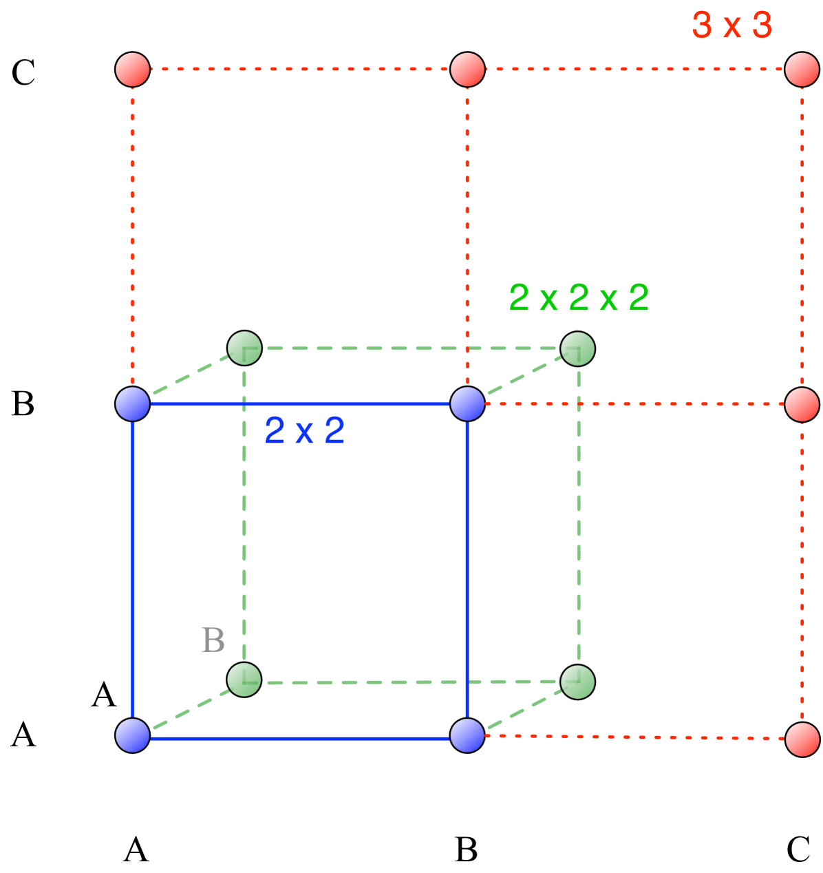
However, for multiplayer games an additional complication arises. Consider a three player game ($d=3$). Let the focal player be playing $A$. As $d=3$ there are $d-1=2$ other players. If one of them is of type $A$ and the other one of type $B$, there can be the combinations $AAB$ or $ABA$. Do these two structures give the same payoffs? Or, in a more general sense, does the order of players matter? If order does matter, the payoffs are in a $d$-dimensional discrete space as illustrated by Fig. 1.

There are numerous examples where the order of the players is very important. In a game of soccer, it is necessary to have a player specialized as the goal keeper in the team. But it is also important that the goal keeper is at the goal and not acting as a centre-forward. A biological example has been studied by Stander in the Etosha National Park stander:1992aa . The lionesses hunt in packs and employ the flush and ambush technique. Some lie in ambush while others flush out the prey from the flanks and drive them towards the ones waiting in ambush. This technique needs more than two players to be successful. Some lionesses always display a particular position to be a preferred one (right flank, left flank or ambush). The success rate is higher if the lionesses are in their preferred positions. Thus, the ordering of players matters here.

To address situations in which the order of player matters, we have to make use of a tensor notation for writing down the payoffs which offers the flexibility to include higher dimensions of the payoff matrix. Consider a tensor $\beta$ with $d$ indices defined as follows $\beta_{i_{0},i_{1},i_{2},i_{3},....i_{d-1}}$, where the first index denotes the focal player’s strategy. Each of the indices represents the strategy of the player in the position denoted by its subscript. The index $i$ can represent any of the $n$ strategies. Thus the total number of entries will be $n^{d}$. This structure is the multiplayer equivalent to a payoff matrix, see broom:1997aa and Fig. 1. Consider for example a game with three players and two strategies ($A$ and $B$). If the order of players matters, then the payoff values for strategy $A$ are represented by $\beta_{AAA},\beta_{AAB},\beta_{ABA}$ and $\beta_{ABB}$. This increase in complexity is handled by the tensor notation but not reflected in the tabular notation Eq. (10). But as long as interaction groups are formed at random, we can transform the payoffs such that they can be written in the form of Eq. (10), see Supporting Text. In this case, the payoffs are weighted by their occurrence to calculate the average payoffs. For example in our three player games, $a_{1}$ has to be counted twice (corresponding to $\beta_{AAB}$ and $\beta_{ABA}$). If we would consider evolutionary games in structured populations instead of random interaction group formation, then the argument breaks down and the tensor notation cannot be reduced.

In case of $d$ player games with two strategies we can then write the average payoff $\pi_{A}$ obtained by strategy $A$ in an infinite population as $\pi_{A}=\sum_{k=0}^{d-1}\binom{d-1}{k}x^{k}(1-x)^{d-1-k}a_{k}$, where $x$ is the fraction of $A$ players. An equivalent equation holds for the average payoff $\pi_{B}$ of strategy $B$. The replicator equation of a 2-player game is given by hofbauer:1998mm

$\displaystyle\dot{x}=x(1-x)(\pi_{A}-\pi_{B}).$

(11)

Obviously, there are two trivial fixed points when the whole population consists of $A$ ($x=1$) or of $B$ ($x=0$). In $d$ player games, both $\pi_{A}$ and $\pi_{B}$ can be polynomials of maximum degree $d-1$, see Supporting Text. This implies that the replicator equation can have up to $d-1$ interior fixed points. In the two strategy case, these points can be either stable or unstable. The maximum number of stable interior fixed points possible are $d/2$ for even $d$ and $(d-1)/2$ for odd $d$, see also hauert:2006fd or broom:1997aa , where it is shown that all these scenarios are also attainable. For $d=2$, $\pi_{A}$ and $\pi_{B}$ are polynomials of degree $1$, hence there can be at most one internal equilibrium, which is either unstable (coordination games) or stable (coexistence games). For $d=3$, there can also be a second interior fixed point. If one of them is stable, the other one must be unstable. This can lead to a situation in which $A$ is advantageous when rare (the trivial fixed point $x=0$ is unstable), becomes disadvantageous at intermediate frequencies, but advantageous again for high frequencies, as in multiplayer stag hunts pacheco:2009aa .

For a $d$ player game to have $d-1$ interior fixed points, the quantities $a_{k}-b_{k}$ and $a_{k+1}-b_{k+1}$ must have different signs for all $k$. However, this condition is necessary (because the direction of selection can only change $d-1$ times if the payoff difference $a_{k}-b_{k}$ changes sign $d-1$ times), but not sufficient, see Supporting Text. Pacheco et al. have studied public goods games in which a threshold frequency of cooperators is necessary for producing any public good pacheco:2009aa ; souza:2009aa . The payoff difference changes sign twice at this threshold value and hence there can be at most two internal equilibria.

A $d$ player game has a single internal equilibrium if $a_{k}-b_{k}$ has a different sign than $a_{k+1}-b_{k+1}$ for a single value of $k$: In this case, $A$ individuals are disadvantageous at low frequency and advantageous at high frequency (or vice versa). If $a_{k}-b_{k}$ changes sign only once, then the direction of selection can change at most once. Thus, this condition is sufficient in infinite populations.

Now we deviate from the replicator dynamics, where the average payoff of a strategy is equated to reproductive fitness, and turn our attention to finite populations. In this case, the sampling for $\pi_{A}$ and $\pi_{B}$ is no longer binomial, but hypergeometric, see Supporting Text. In finite populations, the intensity of selection measures how important the payoff from the game is for the reproductive fitness. We take fitness as an exponential function of the payoff, $f_{A}=\exp(+w\pi_{A})$ for $A$ players and $f_{B}=\exp(+w\pi_{B})$ for $B$ players traulsen:2008aa . If $w\gg 1$, selection is strong and the average payoffs dictate the outcome of the game, whereas if $w\ll 1$ then selection is weak and the payoffs have only marginal effect on the game. This choice of fitness recovers the results of the usual Moran process introduced by Nowak et al. nowak:2004pw and simplifies the analytical calculations significantly under strong selection traulsen:2008aa . However, for non-weak selection other payoff to fitness mappings lead to slightly different results fudenberg:2006fu . We employ the Moran process to model the game, but our results hold for any birth-death process in which the ratio of transition probabilities can be approximated under weak selection by a term linear in the payoff difference in addition to the neutral result. In the Moran process, an individual is selected for reproduction at random, but proportional to its fitness. The individual produces identical offspring. Another individual is chosen at random for death. With this approach we can address the basic properties of $d$ player games with $2$ strategies generalizing quantities from $2\times 2$ games.

Does $A$ replace $B$ with a higher probability than vice versa? Comparing the fixation probabilities of a single $A$ or $B$ individual, $\rho_{A}$ and $\rho_{B}$, we find that $\rho_{A}>\rho_{B}$ is equivalent to

$\displaystyle\sum_{k=0}^{d-1}(Na_{k}-a_{d-1})>\sum_{k=0}^{d-1}(Nb_{k}-b_{0}),$

(12)

see Supporting Text. For $d=2$, we recover the risk dominance from above. For large $N$, the condition reduces to kurokawa:2009aa

$\displaystyle\sum_{k=0}^{d-1}a_{k}>\sum_{k=0}^{d-1}b_{k}.$

(13)

These two conditions are valid for any intensity of selection in our variant of the Moran process.

The one third law for 2-player games is not valid for higher number of players, see Supporting Text. Instead, the condition we obtain for the payoff entries is not directly related to the internal equilibrium points (as opposed to the two player case, which makes the one third law special). For weak selection, we show in the Supporting text that $\rho_{A}>1/N$ is equivalent to

$\displaystyle\sum_{k=0}^{d-1}\left[N(d\!-\!k)-k-1\right]a_{k}>\sum_{k=0}^{d-1}\left[(N+1)(d\!-\!k)b_{k}-(d+1)b_{0}\right].$

(14)

For large population size this reduces to kurokawa:2009aa

$\displaystyle\sum_{k=0}^{d-1}(d-k)a_{k}>\sum_{k=0}^{d-1}(d-k)b_{k},$

(15)

which is the one-third law from above for $d=2$. Inequality (15) means that the initial phase of invasion is of most importance: The factor $d-k$ decreases linearly with $k$ and the payoff values with small indices $k$ are more important than the payoff values with larger indices. Thus, the payoffs relevant for small mutant frequencies determine whether the condition is fulfilled. In other words, the initial invasion is crucial to obtain a fixation probability larger than $1/N$.

In general, the conditions (13) and (15) are independent of each other. When Eq. (13) is satisfied and Eq. (15) is not satisfied then both fixation probabilities are less than neutral ($1/N$). But when Eq. (13) is not satisfied and Eq. (15) is satisfied then both $\rho_{A}$ and $\rho_{B}$ are larger than neutral ($1/N$). This scenario is impossible for two player games.

Let us now turn to multiplayer games with multiple strategies. As illustrated in Fig. 1, the payoff matrix of a two player game increases in size when more strategies are added. If more players are added, the dimensionality increases. Now we address the evolutionary dynamics of such games. Again we assume that interaction groups are formed at random, such that only the number of players with a certain strategy – but not their arrangement – matters. The replicator dynamics of a $d$ player game with $n$ possible strategies can be written as a system of $n-1$ differential equations:

$\displaystyle\dot{x}_{j}=x_{j}(\pi_{j}-\langle\pi\rangle)$

(16)

where $x_{j}$ is the frequency of strategy $j$, $\pi_{j}$ is the fitness of the strategy $j$ and $\langle\pi\rangle=\sum_{j=1}^{n}{x_{j}\pi_{j}}$ is the average fitness. The evolution of this system can be studied on a simplex with $n$ vertices, $S_{n}$. The simplex $S_{n}$ is defined by the set of all the frequencies which follow the normalisation $\sum_{j=1}^{n}{x_{j}}=1$. The fixed points of this system are given by the combination of frequencies of the strategies which satisfy, $\pi_{1}=\cdots=\pi_{n}$. The vertices of the simplex where $x_{j}$ is either equal to $1$ or $0$ are trivial fixed points. In addition, there can be e.g. fixed points on the edges or the faces of the simplex. We speak of fixed points in the interior of the simplex when all payoffs are identical at a point where all frequencies are nonzero, $x_{j}>0$ for all $j$. The internal equilibria are of special interest, because they may represent points of stable biodiversity. For example, three strains of Escherichia coli competing for resources have been studied kerr:2002xg ; czaran:2002ya . $K$ is a killer strain which produces a toxin harmful to $S$, $R$ does not produce toxin, but is resistant to the toxin of $K$. The sensitive strain $S$ is affected by the toxin of $K$. These three strains are engaged in a kind of rock-paper-scissors game. $K$ kills $S$. $S$ reproduces faster than $R$, not paying the cost for resistance. $R$ is superior to $K$ being immune to its toxin. The precise nature of interactions determines whether biodiversity is maintained in an unstructured population hofbauer:1998mm ; claussen:2008aa . In our context this is reflected by the existence of an isolated internal fixed point.

Here, we ask the more general question whether there are internal equilibria in $d$ player games with $n$ strategies. If so, then how many internal equilibria are possible? It has been shown that for a two player game with any number of strategies $n$ there can be at most one isolated internal equilibrium hofbauer:1998mm ; bishop:1976aa . In the Supporting Text, we demonstrate that the maximum number of internal equilibria in $d$ players with $n$ strategies is

$\displaystyle(d-1)^{n-1}.$

(17)

The maximum possible number of internal equilibria increases as a polynomial in the number of players, but exponentially in the number of strategies. For example for $d=4$ and $n=3$ the maximum number of internal equilibria is 9, see Fig. 2.

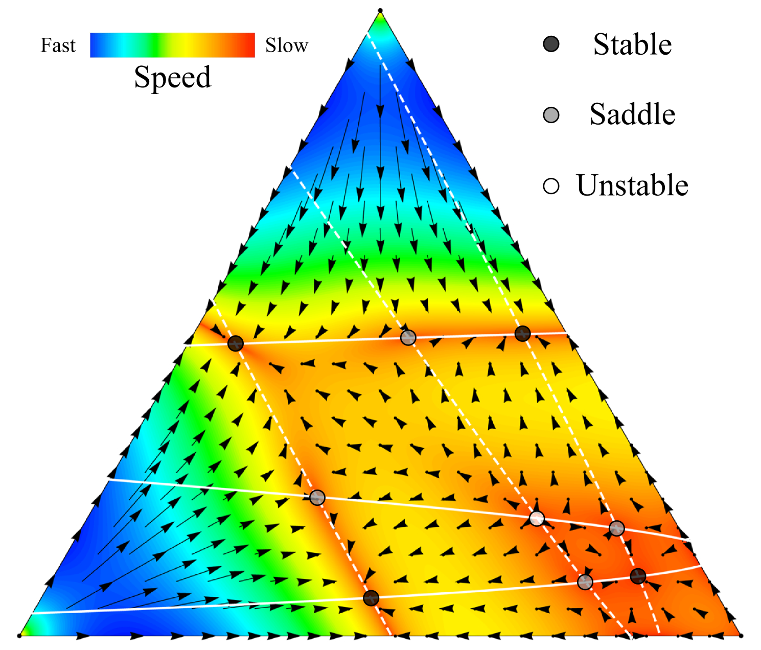
Note that for $d=2$ we recover the well known unique equilibrium. For $n=2$, we recover the maximum of $d-1$ internal equilibria, see above. Of course, not all of these equilibria are stable. Broom et al. have shown which patterns of stability are attainable for general 3-player 3-strategy games broom:1997aa .

This illustrates that many different states of biodiversity are possible in multiplayer games, whereas in two player games, only a single one is possible. This is a crucial point when one attempts to address the question of biodiversity with evolutionary game theory. In the previous example the studies dealing with E. coli consider the system as a $d=2$ player game with three strategies. Do we really know that $d=2$? If strains are to be engineered to stably coexist, then multiple interactions ($d>2$) would open up the possibility of multiple internal fixed points instead of the single one for $d=2$.

If we choose a game at random, what is the probability that the game has a certain number of internal equilibria? To this end, we take the following approach: We generate many random payoff structures in which all payoff entries are uniformly distributed random numbers huang:2010aa . For each payoff structure, we compute the number of internal equilibria. It turns out that games with many internal equilibria are the exception rather than the rule. For example, the probability to see $2$ or more internal equilibria in a game with $4$ players and $3$ strategies is $\approx 24\%$. The probability that a randomly chosen game has the maximum possible number of equilibria decreases with increasing number of players and number of strategies, see Fig. 3.

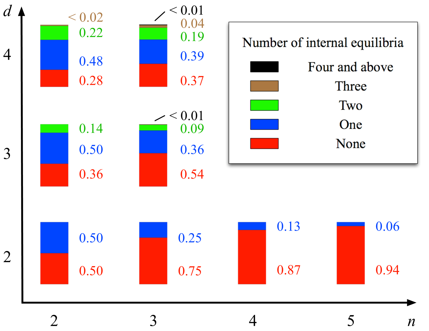
Also the probability of having a single equilibrium reduces. Instead we obtain several internal equilibria in the case of more than two players. For two player games, the probability to see an internal equilibrium at all decreases roughly exponentially with the number of strategies. This poses an additional difficulty in coordinating in multiplayer games, because several different solutions may be possible that look quit similar at first sight.

Multiplayer games with multiple strategies is what we find all around. We interact with innumerable people at the same time, directly or indirectly. Some interactions may be pairwise, but others are not. In real life, we may typically be engaged in many person games instead of a disjoined collection of two person games hamilton:1975aa . The evolution and maintenance of cooperation, problems pertaining from group hunting to deteriorating climate, all are fields for a multiple number of players stander:1992aa ; levin:2009aa ; milinski:2008lr ; broom:2003aa . They can have different interests and hence use different strategies. There are other cases like the maintenance of biodiversity where multiplayer interactions may lead to a much richer spectrum for biodiversity than the commonly analyzed two player interactions. The presence of multiple stable states also contributes to the intricate dynamics observed in maintenance of biodiversity levin:2000aa . Multiplayer games may help to improve our understanding of such systems. The problem of handling multiple equilibria is not just limited to biological games but it also appears in economics kreps:1990bo ; damme:1994aa . Many insights can be obtained by studying two player games, but it blurs the complexity of multiplayer interactions. Here, we have derived some basic rules which apply to multiplayer games with two strategies for finite as well as infinite populations and discussed the number of internal equilibria in $d$ player game with $n$ strategies, which determine how the dynamics proceeds.

This theory can be applied to all kinds of games with any number of players and strategies and can thus be easily applied to public goods games, multiplayer stag hunts or multiplayer snowdrift games. We believe that this opens up new avenues where we can get analytical description of situations which are thought to be very complex and further discussions on these issues will prove to be fruitful due to the intrinsic importance of multiplayer interactions. We conclude this approach by quoting Hamilton again, “A healthy society should feel sea-sick when confronted with the endless internal instabilities of the ‘solutions’, ‘coalition sets’, etc., which the theory of many-person games has had to describe.” hamilton:1975aa .