Evolving Network Model that Almost Regenerates Epileptic Data
Abstract
In many realistic networks, the edges representing the interactions between the nodes are time-varying. There is growing evidence that the complex network that models the dynamics of the human brain has time-varying interconnections, i.e., the network is evolving. Based on this evidence, we construct a patient and data specific evolving network model (comprising discrete-time dynamical systems) in which epileptic seizures or their terminations in the brain are also determined by the nature of the time-varying interconnections between the nodes. A novel and unique feature of our methodology is that the evolving network model remembers the data from which it was conceived from, in the sense that it evolves to almost regenerate the patient data even upon presenting an arbitrary initial condition to it. We illustrate a potential utility of our methodology by constructing an evolving network from clinical data that aids in identifying an approximate seizure focus – nodes in such a theoretically determined seizure focus are outgoing hubs that apparently act as spreaders of seizures. We also point out the efficacy of removal of such spreaders in limiting seizures.
Keywords: Mathematical modeling, time-varying network, state forgetting property, focal epilepsy, discrete-time dynamical system, nonautonomous dynamical system
1 Introduction
Increasingly, many complex systems are being modeled as networks since the framework of nodes representing the basic elements of the system and the interconnections of the network representing the interaction between the elements fits well for a theoretical study. When the complex systems are large-dimensional dynamical systems, the network framework comprises many interacting subsystems of smaller dimension each of which constitutes a node. As a particular example, the whole or a portion of the entire neuronal activity in the human brain can be regarded as the consequential dynamics of interacting subsystems, where the dynamics of a subsystem is generated by a group of neurons. The enormously interconnected subsystems in the brain generate a wide variety of dynamical patterns, synchronised activities and rhythms.
Epilepsy is a disorder that affects the nerve cell activity which in turn intermittently causes seizures. During such seizures, patients could experience abnormal sensations including loss of consciousness. Clinical and theoretical research have shown that underpinning the cause of this disorder has not proved to be easy, in particular the predicament of resolving the question as to whether the disorder manifests due to the nature of the interconnections in the brain or the pathologicity of a portion of the brain tissue itself remains.
Since epilepsy is one of the most common neurological disorders with an estimate of more than 50 million individuals being affected [26], there is a strong need both for curative treatment and as well for the analysis of the underlying structure and dynamics that could bring about seizures. In this paper, our attention is on focal epilepsy where the origin of the seizures are circumscribed to certain regions of the brain called the seizure focus [4, 3, 7, 19, 27, 32, 36], and the aim of this paper is to foster theoretical investigation into the connection strengths of the underlying nodes in such a seizure focus in comparison to the other nodes in the network.
Different models have been proposed to understand different aspects of focal epilepsy [1, 13, 38]. Mathematically speaking, dynamical system models of focal epilepsy studied in the literature are mainly of two broad categories: (i). Models that consider noise to be inducing seizures in a node [15, 31, 34] (ii). Models that consider seizures to be caused or terminated by a bifurcation, a change in the intrinsic feature of the (autonomous) dynamics at the node [5, 24, 28].
While modeling the neuronal activity of the human brain, there are far too many numerous parameters which also dynamically evolve on separate spaces and scales, and it is unrealistic to observe or encapsulate all these aspects in a static network or an autonomous dynamical system (see Appendix A). Since the brain evolution does not depend on its own internal states as it responds to external stimuli and the interconnections in the brain are likely to change in response to stimuli, the human brain can be safely said to be a nonautonomous system and in the language of network dynamics, this is effectively an evolving network (see Section 2).
Besides evidence that network connections play a role in initiating seizures (e.g., [2, 4, 20, 32]), some authors also provide evidence that stronger interconnections play a role in epileptic seizures (e.g., [11, 25]). Also, a commonly found feature of biological systems is adaptation: an increase in exogenous disturbance beyond a threshold activates a change in the physiological or biochemical state, succeeded by an adaptation of the system that facilitates the gradual relaxation of these states toward a basal, pre-disturbance level. Based on all these, we present a novel phenomenological model where seizures could be activated in a node, if certain interconnections change to have larger weights resulting in a larger exogenous drive or disturbance or energy transmitted from other nodes into it, and upon experiencing seizure, adjustment of interconnections takes place eventually to subside the seizures. Since the interconnections are allowed to change, the model dynamics emerges from an evolving network.
In this paper, we propose a patient and data-specific, macroscopic, functional network model that can act as a “surrogate” representation of the electroencephalography (EEG) or electrocorticography (ECoG) time-series. The network model is new in the sense that it satisfies the following simultaneously: the network connections are directed and weighted; the network connections are time-varying; there is a discrete-time dynamical system at each node whose dynamics is constantly influenced by the rest of the network’s structure and dynamics; the ability of the network to generate a time-series that sharply resembles the original data is based on a notion of robustness of the dynamics of the network to its initial conditions what we call as the “state-forgetting” property.
The essence of the state-forgetting property, roughly put is that the current state of the brain does not have an “ distinct imprint” of the brain’s past right since from its “genesis” or “origin” (rigorous definitions are provided later in the paper). Effectively, this means that the brain tends to forget its past history as time progresses. Such a notion has been adapted from the previously proposed notions for studying static (artificial neural) networks with an exogenous input in the field of machine learning viz., echo state property [12, 22], liquid state machines, [21], backpropagation-decorrelation learning,[33] and others. However, the network model that we represent is very different from that of the artificial neural networks and moreover the nodes in our model correspond to different regions of the brain.
Our methodology is as follows: We present an evolving network model which exhibits state-forgetting property for all possible inter-connections, and a particular sequence of interconnection strengths (matrices) is determined from a given EEG/ECoG time-series so that the model can almost regenerate the time-series. The weights of the interconnections are chosen from a set of possibilities based on a heuristic algorithm that infers a causal relationship between nodes – a (directed) synchrony measure between two nodes and represents the conductance (ease at which energy flows) from node into node , and weight of the connection from node into node has some degree of proportionality with the synchrony measure.
The state forgetting property ensures the synthesized evolving network has in some sense captured the original time series as an “attractor” (see [23] and Proposition C.1), and hence the network acts as surrogate representation of the original time series. In other words, since any initial condition presented to a state-forgetting network has no effect on its asymptotic dynamics, and that the asymptotic dynamics resembles the time-series, we assume that the evolving network model has captured the essence of the time-series data.
To indicate the potential utilities of the model, we analyse the constructed evolving network from a patient’s clinical data. By comparing the relative strength of the interconnections, we identify nodes that are outgoing hubs of the network as a theoretically determined seizure focus. The nodes in such a focus have a strong location-wise correlation with the set of nodes in a clinically determined seizure focus. We also, discuss the efficacy of surgical removal of the determined focus in subsiding seizures.
The remainder of the paper is organised as follows. We introduce the notion of state-forgetting evolving networks in Section 2; formal definitions are made in Appendix B. In Section 3, we present the evolving network model in detail and state a result concerning the state-forgetting property; the complete mathematical proof of this result is presented in Appendix C. In Section 4, we present a method to obtain the weight matrices to obtain a time-varying network from a clinical time series. In Section 5, we present some results on the network inference followed by a brief discussion and conclusion in Section 6.
2 Evolving networks that are state-forgetting
The aim of this section is to give an intuitive description of the state forgetting property of evolving networks; the formal and rigorous definitions of this property are found in Appendix B. We employ discrete-time systems [6] since they are more amenable to computer simulations as the computed orbits or solutions unlike in the case of differential equations do not depend on numerical methods for computing the solutions and their related accuracy. Also, discrete-time systems can exhibit complex dynamical behaviour (e.g., [6]) even in one-dimension whereas a continuous time-system needs a dimension of at least three.
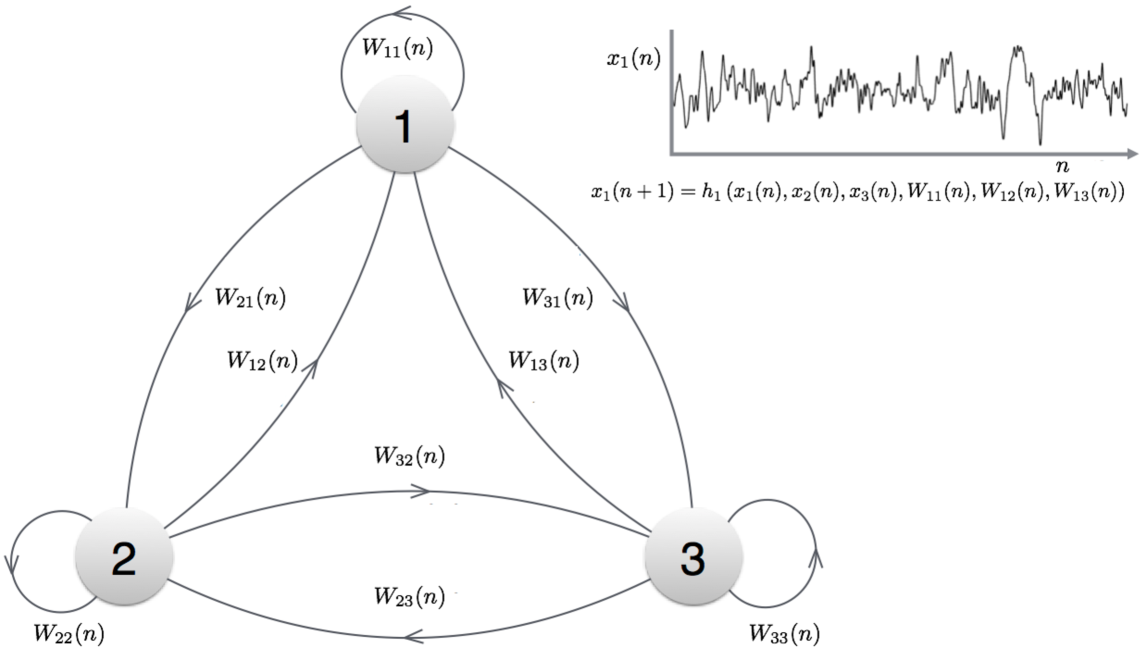
Using Fig. 1, we present a less formal and simplistic description of an evolving network with three nodes . Let be a matrix defined for each integer with being the strength of the incoming connection from node to node ; here is the element in the row and column of . There is a discrete-time dynamical system at each node in the evolving network represented in Fig. 1, and the node dynamics is given by
where is some function (not dependent on ) that calculates using information from the dynamical state in the three nodes at time and the respective incoming strengths into node . By specifying , and together with the sequence of weight matrices , the evolving network is specified completely. By denoting , we can represent the evolving network dynamics also as a nonautonomous system , where the variation of with represents the inherent plasticity of the system (change in above). We can also allow ’s to represent external stimuli to the network and other obfuscated factors.
Since an evolving network is essentially a nonautonomous system, we recall some relevant results of a nonautonomous system. Of interest to us is the notion of an entire-solution of a nonautonomous system. An entire solution (or orbit) of a nonautonomous system is a sequence that satisfies for all . It is possible to show under natural conditions that there exist at least one entire solution [22]. In the particular case, where the evolving network has a unique entire solution, we say that the network (or the nonautonomous system) has the state-forgetting property (formally defined in Definition B.2).
Now, we comment on the rather intriguing consequence of an evolving network having multiple entire-solutions. Suppose and are two distinct entire-solutions of a nonautonomous dynamical system, then for some time , we have i.e, the system could have evolved into two possible states at time . Since and , it is necessary to have . Similarly, would necessitate and so on. Thus, in general, at any time-instant , implies that there are two entire-solutions that have had distinct infinitely long pasts. In other words, the dynamics of such systems with distinct entire-solutions “depends” not only on the inherent plasticity or the exogenous stimuli represented by the maps , the distinct solutions carry a distinct and non-vanishing imprint of their past.
From the arguments in the preceding paragraph, for nonautonomous systems like the human brain, having more than one entire solution translates to saying that the current state of the brain is not just the result of the changing interconnections in the brain or the exogenous input but to also say that its past states have a non-vanishing effect on the asymptotic dynamics.
Since it is hard to envisage or believe that seizures in current time had something to do with the state of the brain right from its “genesis” (genesis is used as a metaphor to refer to the earliest factual time instant from which the current brain state has evolved from, and this time could be matter of debate), we assume the more plausible – seizures at a certain time are a consequence of how the network structure has evolved/changed till that time or a result of a stream of exogenous inputs to the brain, but certainly not a consequence of the state at which the brain was in during its genesis. This also forms the basis for employing echo-state networks in artificial neural network training and machine learning[12, 22].
Whenever a nonautonomous system (technically, defined on a compact state space) has the state-forgetting property, it also has state-space contraction towards its entire-solution in the backward direction (see Proposition C.1). In fact, a stronger result [23] holds: if is the unique entire solution, then for every the successive iterates would satisfy as . In other words, “attracts” all other state-space iterates towards it (component-wise) as time tends to infinity. This convergence due to the attractor property of the state-forgetting property is what makes our evolving network model generate a time-series that actually sharply resembles (mathematically, converges to) the data from which the network was conceived. Further discussion on attractivity is beyond the scope of this paper. The larger point is that for an evolving network to be of utility as a surrogate representation of the time-series data, we need the state-forgetting property.
3 Model
Before, we actually describe the evolving network model in (23), we list and describe its features: (i). The evolving network model has -nodes for all time. (ii). Placed at each node is a certain bi-parametric one-dimensional discrete-time dynamical system which is autonomous when there are no incoming connections from other nodes to it, and nonautonomous otherwise. We refer to the dynamics of the system at a node, as the dynamics of the node or nodal dynamics. (iii). Among the two parameters that specify this one-dimensional dynamical system is a stability parameter. The nodal dynamics in autonomous mode has a globally stable fixed point at whenever the stability parameter is in a certain range (stable-regime); a globally stable fixed point attracts all solutions, i.e, the time series values measured in the node are close to and tend towards to it. (iv). When the stability parameter is chosen not to lie in the stable regime, the autonomous nodal dynamics can render a range of different behaviours including oscillatory behavior, complex behavior like chaos [6] depending upon the value of the stability parameter. (v). When the nodal dynamics is nonautonomous, the dynamics of the node is perturbed at each time-instant from the dynamical states of other nodes. We call the net perturbation from other nodes as the drive to the node under consideration. The exogenous drive from other nodes has its signature on the nodal dynamics, and if sufficiently strong, is also capable of setting the nodal dynamics far away from the fixed point . (vi). We term a seizure in the node to be a dynamical excursion away from the fixed point, and that the seizures in a node are brought about (and terminated) in two distinct scenarios: (via). changing the stability parameter of the node in the autonomous mode of operation (vib). by the nature of the exogenous drive from the other nodes in the network in the nonautonomous mode. (vii). In this paper, we consider the case of nodal dynamics slipping into seizures as in scenario (vib) above, i.e, we consider each node to have its stability parameter to lie in the stable regime, and the exogenous drive to cause seizures. The drive is time-varying on two accounts: first, being a function of the states of the other nodes it is time-varying as other nodes have a dynamical system and not static; second, the drive is time-varying since it is a function of the interconnection strengths of the nodes.
Our model is also motivated on the lines of previous research [14, 30, 35, 37] showing that the hyper-interconnected regions in the brain are prone to seizures (see Section 3). Hence, we expect the drive to an individual node is likely to be having large magnitude if it has large weighted incoming connections.
To describe a family of evolving networks (as in Definition B.1), we first sketchily describe the nonautonomous dynamics at each node (the map described in Section 2 or in Definition B.1) via the update equation:
| (18) |
where the various entities are listed and briefly explained:
-
•
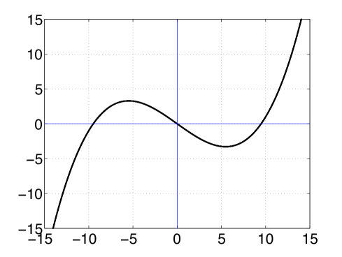
The iteration of the map on an initial condition gives the autonomous dynamics of the node. Some Neuron models like that of Fitzhugh-Nagumo (e.g., [9, 29]) permit an individual neuron to have a regenerative self-excitation via a feedback term. Based on this principle, we consider a highly simplistic discrete time model of the node dynamics where feedback from the node dynamics can cause self-excitation, and set
(19) where parameters and (for a graph of , see Fig. 2(a)). Explanation on how a parameter can cause self-excitation dynamics is made in Section 3.1.
-
•
Adopting the principle that the individual drive from a connecting node has a larger magnitude if the incoming connection weight and the magnitude of the state value of the connecting node are together larger, we set the total sum of the drives from the other nodes into the node to be
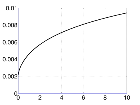
(20) where is the weight of the incoming connection from the node to the node; is an offset parameter to enable a positive argument for the function; is an increasing function and is defined by
(21) The function although increasing, has a monotonically decreasing slope (see Fig. 2(c)). The net effect of the function can be thought of as the node’s mechanism to have a relatively stronger inhibition to a stronger incoming connection – node’s internal mechanism to resist seizures by inhibiting stronger exogenous drive. Lastly, the negative sign in (20) is only for mathematical convenience and has no physical significance. When the drive is zero, the dynamics of the node is in autonomous mode.
-
•
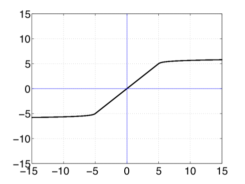
The saturation function henceforth would be the mapping which is linear in a certain adjustable range, and its slope becomes zero asymptotically (see Fig. 2(b)) defined by:
(22) where and is the identify function on ; determines the asymptotic rate at which the slope of decreases and . (see Fig. 2(b)); is linear in the region with a slope , and the slope of approaches as monotonically according to .
Putting together the above into (18), the update equation at the node is modeled by:
| (23) |
Note that in the model in (23), the weights are unspecified, but they actually can be solved for given a ECoG/EEG time-series (topic of Section 4). In Section 3.1 and 3.2, we describe the dynamics of a node when it operates in autonomous node and in the nonautonomous mode. In Section 3.3, we state sufficient conditions on the parameters , and , to ensure state-forgetting property of any evolving network arising out of (23). However, to understand the model, a few remarks are in order concerning the role of the offset parameter and the saturation function in (23):
From (20), it follows that the individual drive from the node into node , at time is given by . To make the role of the weights meaningful, a smaller weight should ensure smaller individual drive from node , i.e., we must have close to zero whenever is close to zero. We note that this would be the case whenever the offset parameter is sufficiently large. To observe this, we remark on the behavior of as the weight gets close to zero. By definition of in (21), when is close to zero, it follows that is close to . When is close to , is close to . For practical purposes we restrict (see Section 4), and hence if is much larger than , then is close to , and is close to zero, and thus is very close to zero. However, it is also to be noted that if is made unreasonably large, the signature of on gets weaker, so is chosen in an appropriate range, although with a large value. Physiologically, the parameter has no direct relation, but serves as a mathematical plug to overcome the difficulty in modeling the drive directly from the dynamical states of a connecting node that take both positive and negative values. The offset has another role: its value could determine the state-forgetting property of an evolving network (see Theorem 3.3.1).
The particular choice of the saturation function is not critical to the model; for the convenience of mathematical proofs, we need to be differentiable and unbounded and hence its form. On the other hand, for practical reasons, choosing such a , helps in the simulation stage to troubleshoot if each of the parameters , and are chosen in an appropriate range lest the network lose the state-forgetting property. While the network does not have the state-forgetting property, the dynamics can be unbounded in the absence of a saturation function since the range of is unbounded and the numerical values on a computer could indicate an error.
3.1 Isolated node-dynamics
We present a short summary of the dynamics of the family of maps described in (19). The detailed analysis of this family of maps is not the subject matter of this paper, and the discussion here is only intended to convey the point that the dynamics of adds notable features to the evolving network model. Recall that the parameters are restricted to and . With , it can be easily verified that there is an invariant closed interval symmetrically extending on either side of the real number given by , i.e., . The dynamics of on is relevant to us since the dynamics outside escapes to . With fixed, and increasing through to , the dynamics of this family of maps on takes a route to chaos qualitatively similar to the variation in from to in the well studied logistic family of maps on (for e.g., [6]). Elaborating this further, when , the fixed point is globally stable, in the sense that every orbit asymptotically approaches the fixed point as tends to ; when , the fixed point loses stability and undergoes a period doubling bifurcation. As is increased beyond , period doubling cascades occur alike in the logistic family of maps [6], and eventually there is a transition to chaos. Thus each node has the potential to have self-excitatory dynamics (oscillate or exhibit complicated behaviour) if the stability parameter for the node is set between .
3.2 Driven node-dynamics
Adding a time varying drive to the update equation of by
makes the mapping depend on , and clearly the graph of such a mapping at any is a vertically shifted version of the graph of Fig. 2(a) with the shift determined by . Since, we expect to be changing with every , the stable fixed point dynamics is not a feature of nonautonomous dynamics. As mentioned above, increasing beyond , makes the dynamics move away from the fixed point at . We make use of the fact that to move the nonautonomous dynamics away from the fixed point, it is not necessarily required to increase beyond , but a sufficiently strong drive is capable of moving the dynamics. Also, some background observations and computer simulations suggest that larger the magnitude of drive, further away is the likelihood of the dynamics away from .
3.3 Is the evolving network state-forgetting?
Having made some points on the nodal dynamics, we now state a result on the evolving network. Next, we state a theorem which says that when is sufficiently large, then any evolving network obtained from (22) is state-forgetting. The complete proof of this result is provided in Appendix C.
Theorem 3.3.1
Fix non-zero, positive reals such that the following hold
4 Heuristic algorithm: directed weights from EEG/ECoG time-series
Henceforth, for ease of jargon we call the component of a -dimensional time series data , i.e., the data in the channel. Given , we present a method for solving the weights in(23) based on inferring a causal relationship between the nodes, which we call a synchrony measure.
To explain the methodology of solving weights from (23), we rewrite (23) by rearranging as
| (24) |
where is the inverse of the saturation function . Clearly, given a -dimensional time-series of EEG or ECoG clinical data, and having fixed , in the model, the right hand side of (24) can be computed easily for each from the channel data. Let denote the right hand side term in (24).
For a fixed , we have a single equation
| (25) |
where there are unknown quantities as is varied from to with . Hence, multiple solutions of could exist since we have more unknowns than equations. We regard seizure spread in the network due to sustained energy transmitted from a node that is seizing to the ones which is not. With this principle, we hypothesize to be an increasing parametric function of a certain synchrony measure between the two distinct nodes and . Physiologically, the synchrony measure between two nodes and represents the ease at which energy dissipates (a measure of conductance) from node into node , and hence is directed – nodes and could have different interconnections, and energy dissipation between nodes is not symmetric. To get a measure of such conductance, we let the synchrony measure depend on (i) a sustained influence from node into node measured by a leaky integrator placed between the two nodes (ii) the similarity between the average amplitude or power in the two channels up to time .
The algorithm for computation of directed synchrony between two channels is described in Section 4.1. We now explain the idea/reasoning behind some of the steps of the algorithm. The discussion can be read in conjunction with the various steps of the algorithm.
The very first step of the algorithm involves normalisation of the amplitude of data for setting the amplitude of the time-series in any channel lies between (see (S1) of Section 4.1).
In a succeeding stage of the algorithm, we compute the average power at each instant in a window of length in each channel (see definition of in (S6) of Section 4.1). It turns out that the time interval in which there is sustained influence of one node on the other by the synchrony measure is determined by . We comment on the choice of in Section 5.1
The directed synchrony depends on the product of two factors (see (S7) of Section 4.1). One of the factors is the similarity between the powers in the and channels which we quantify by a similarity index . Note that due to normalisation in (S1), the average power in any window is between and , and hence , and the similarity index attains if and only if and are identical.
The other factor that contributes to is , the output of a (directed) nonlinear leaky integrator placed between two distinct nodes and whose states are evaluated recursively (for details see (S8) to (S12) of Section 4.1)). The purpose of such a leaky integrator is to model the sustained influence of the signal strength in the node on node – the word sustained points to the fact that the integrator leaks, and unless the influence is not sustained over a period of time, the influence diminishes. Any such leaky integrator in (S11) of Section 4.1 is a nonautonomous dynamical system in its own right, and hence its future states are obtained by iteration on the current state. In essence, a leaky integrator sums up (or integrates) its previous state with what is fed to it typically as an input, but also leaks a small fraction of the sum while integrating. Here, we set the leaky integrator dynamics for the connection from node to as
where the cumulative average power in the channel is calculated as in (S9) of the algorithm. This cumulative average fractional power is determined by first calculating the fractional power in the channel (see (S8) of the algorithm). The cumulative average of this fractional power is calculated as in (S9) of the algorithm; this cumulative average is calculated iteratively using the elementary idea: to calculate the average of a collection of numbers , if the average of numbers is given to be , then the average of numbers can be updated by .
Once the synchrony from the time series from the algorithm in Section 4.1 is computed, then for convenience, we proceed to deduce the intermediate quantity from which the actual weight can be readily obtained (see (28)).
We hypothesise to be an increasing parametric function of and is in the form
| (26) |
where the parameter can be solved as explained below. Substituting in Eq. (25), we have the following straightforward deduction to get an expression for :
| (27) |
Once is found, the weight can be easily found since is invertible. From (21), we get
| (28) |
4.1 Algorithm to find the synchrony
The algorithm is described in the following ordered steps (S1) to (S12).
-
(S1).
Normalize or scale the time-series data , by dividing each component in each channel by so that upon normalisation the time-series satisfies: (i) every value of the time series in each channel lies between (ii) the maximum of absolute value of the normalised time-series (retaining the same notation as the original time-series) is , i.e., .
-
(S2).
Fix the parameters , and of the network, and a large positive integer . It is suggestive that the parameters and are chosen to satisfy , and . Once these values are fixed, (by Theorem 3.3.1) the value of the parameter determines the state-forgetting property of the evolving network. The state-forgetting property can be cross-verified after simulations (see Figure 3); the minimum value of required increases with the number of nodes in the network. For instance, in our simulation results in Section 5, with , the value of is found to be sufficient for the network to satisfy the state-forgetting property when , and .
-
(S3).
For all time , initialise the cumulative average power in each of the channel to be .
-
(S4).
At time , initialize, the leaky integrator state a random number for all .
-
(S5).
Set a counter to an initial state, (to aid a calculation in (S9)).
-
(S6).
Obtain the average power in every channel of the time series at the time instant using the data in the window as (Note: Clearly, since the data is normalized in (S1), )
-
(S7).
Define the directed synchrony for all , running from with .
-
(S8).
Find the fraction of the power in each channel , using
-
(S9).
For each , compute the cumulative average of the fractional power from and using
-
(S10).
Denote , the quantity that is to be fed into the leaky integrator to obtain its next state.
-
(S11).
The function when shifted up and to the right is a positive increasing map on with a large slope in a very short interval; we use such a function to update the leaky integrator state according to
-
(S12).
If needs to be computed, set ; , and return to (S6).
We recapitulate from Section 2, that only a state-forgetting network can attract all other iterates towards a unique entire solution. As a numerical verification of this, in Section 5 we show the ability of the evolving network model to generate a time series from an arbitrary initial condition that begins to resemble the original one in a very few time steps.
5 Network Inference & Potential Utility
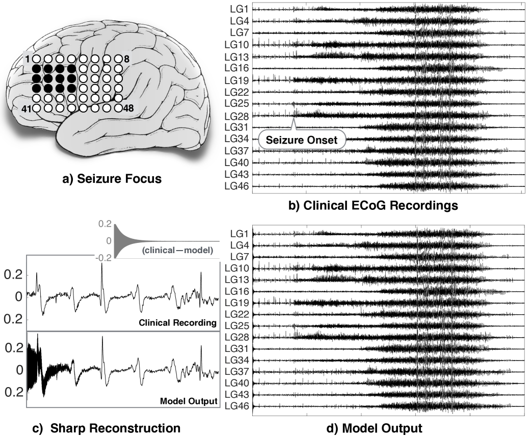
We infer cortical connectivity from a 58 year old male patient diagnosed at Mayo Clinic. The patient had intractable focal seizures (seizures that fail to come under control due to treatment) with secondary generalization (seizures that start in one area and then spread to both sides of the brain). The patient underwent surgical treatment and pre-surgical evaluations were performed using a combination of history, physical exam, neuroimaging, and electrographic recordings. For delineating the epileptogenic tissues, electrocorticography (ECoG) recording was performed at a sampling frequency of 500 Hz for four days continuously with grid, strip, and depth electrodes implanted intracranially on the frontal, temporal and inter-hemispheric cortical regions. A total of nine seizures were captured during the recording period and complete seizure freedom was achieved (ILAE class I) following the resection of pathological tissues in the left medial frontal lobe and medial temporal structures. All recordings were performed conforming to the ethical guidelines and under the protocols monitored by the Institutional Review Board (IRB) according to National Institutes of Health (NIH) guidelines. The clinical data and ECoG recordings for this patient are publicly available on the IEEG portal (https://www.ieeg.org) with dataset ID ‘Study 038’.
In our analysis, we consider only the electrodes in the grid placed on the frontal lobe where both the seizure onset and its spread were captured. The electrodes which circumscribed the epileptogenic tissues are shaded in black on the schematic shown in Fig. 3(a). A small segment of ECoG recording is sufficient to demonstrate the efficacy of our modelling framework. Therefore, we select an ECoG segment comprising of both pre-ictal and ictal activities to explore how the network evolves during seizures. We remove the noise artefacts and the power-line interference from the raw ECoG signals by applying a bandpass filter between Hz and a notch filter at Hz. The ECoG signals from a few exemplary electrodes (labeled with a prefix LG) are shown in Fig. 3(b).
Next, we infer an evolving network synthesized from the ECoG data. We consider the cortical area under each ECoG electrode as a network node and apply algorithm detailed in Section 4.1 to get the directed and weighted edges or interconnections between the nodes so that (23) is satisfied. In particular with parameters , , , we apply the algorithm to obtain the weights of the interconnections between the nodes at each time sample of the data. To cross validate that the weights obtained eventually render a state-forgetting evolving network, we adopt the following procedure. With an arbitrary initial condition and the obtained weights at time , we use (23) to obtain . Repeating this, we obtain , and so on. The time-series in a few channels obtained from this procedure is shown in Fig. 3(d). Apparently, the time-series in Fig. 3(b) and Fig. 3(d) are similar. Actually, the similarity is true barring a few hundred samples at the beginning (see Fig. 3(c)). This convergence of the model output from an arbitrary initial condition to the given time-series verifies state-forgetting property and validates our modelling framework for the study of network evolution during seizure onset and seizures.
As a passing remark to the reader, the model’s ability to sharply reconstruct the given data as indicated in Fig. 3(c) (plots of the first 2000 samples of an ECoG channel data, corresponding model output and their difference) is robust even for a different choice of parameters in the algorithm. In fact, Theorem 3.3.1 tells us that such a reconstruction is possible as long as the parameters are in a certain range.
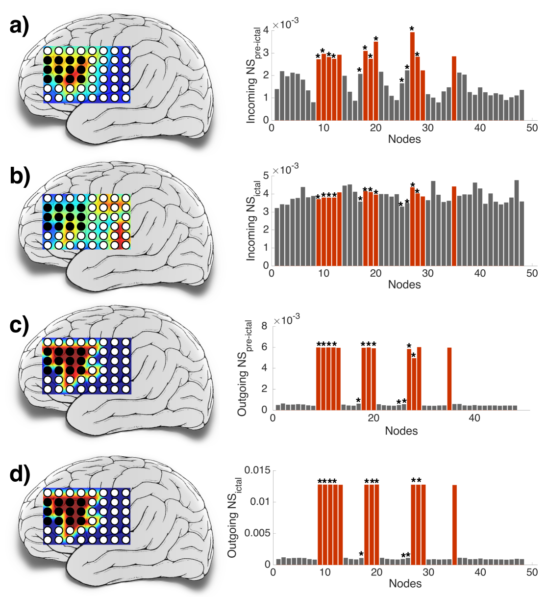
With an objective of identifying the nodes crucial for the seizure genesis, we study the network properties before and after the seizure onset. Consequently, we divide the ECoG recordings into two segments: pre-ictal (before seizure onset) and ictal (after seizure onset).
For each segment of this data, we compute an ensemble average of node strengths as explained next. It may be recalled from Section 3 that the drive from node to at time is given by . For each node , we compute its mean incoming drive strength of node over a time period as where is the number of nodes, and is the number of sample points in . In a similar vein, we compute the mean outgoing drive strength of node over a time period as
Figure 4 shows the mean incoming and outgoing node strengths for each node during the pre-ictal and ictal periods. Fig. 4 (a) indicates a strong correlation of the mean incoming node strengths with the clinical seizure onset zone or seizure focus (depicted by the electrodes shaded in black) during the pre-ictal period, while Fig. 4 (b) indicates a more uniform spread of mean incoming node strengths across all nodes during the ictal period. The correlation of the mean incoming node strengths with the clinical seizure onset zone during the pre-ictal period can be understood as that the external drives from other nodes play a supportive role in initiating seizures (a hypothesis of our model as well). Since during the ictal period all channels seem to have similar average power due to seizures, all nodes are likely to receive a similar quantum of external drive. Hence, the mean incoming drive strength appears to be uniform.
In contrast, Fig. 4 (c, d) shows that the distinctively higher mean outgoing node strength (during both ictal and pre-ictal period) is much strongly “correlated” with the clinical seizure onset zone than that shown by the corresponding mean incoming node strengths. Therefore, from Fig. 4 (c, d), it is evident that the nodes whose node strengths are shown as columns in red (i.e., nodes ) are the outgoing hubs. We refer to this set of nodes as the theoretical seizure onset zone.
Incidentally in this experiment there are 12 nodes in the theoretical seizure onset zone, similar in cardinality to the set of the nodes at the site of clinical resection ( i.e., nodes ). We refer to the nodes at the site of clinical resection as the clinical seizure onset zone. It is evident that the theoretical seizure onset zone and the clinical seizure onset zone point to very similar regions in the brain. Thus, the model has the potential utility of identifying an approximate seizure focus zone prior to surgery by analysing some pre-ictal and ictal data.
Although the theoretical and clinical onset zones differ slightly, from a theoretical standpoint of view, we can hypothesise the outcome of the surgical removal of these two zones and compare these outcomes if we have a suitable objective measure. To explain this, let be the indices of the subset of the nodes that are omitted from a network of nodes in a simulation experiment, i.e, the nodes in are made non-functional by setting for all if either or belongs to . Using such modified weight matrices in (23) we can obtain a time-series of the depleted network can be calculated by starting with any initial condition that satisfies whenever . In other words, the signal has to have zero amplitude in all the channels corresponding to the nodes in since they are assumed to not participate in the network dynamics.
We quantify the efficacy of the removal of the nodes that belong to by calculating the ratio of the average power in those channels outside prior to removal of nodes and after it by:
where denotes the number of samples over a time-interval and denotes the cardinality of the set . Similarly the average power in the signal generated from the depleted network can be calculated by and we calculate the efficacy of removing the nodes by the ratio
We tabulate the values of below, where is determined by the following choices: (i) the clinical seizure onset zone (ii) theoretical seizure onset zone (outgoing hubs) (iii) an arbitrary set of 12 nodes (iv) 12 nodes randomly drawn (average of is tabulated in this case). Now, we discuss the potential application of the model in a clinical study when surgery is part of the treatment. The aim of a clinical surgery would be to a minimise the removal of tissue from the brain along with subsiding seizures post surgery. In our study above, the removal of a set of nodes from the evolving network is intended to simulate a surgical removal of the tissue beneath the nodes in . A time series from the depleted network is intended to simulate the resultant clinical ECoG time series observed after surgery, and the quantity is meant to measure the efficacy of the surgery. Thus prior to an actual surgery, the theoretical efficacy of surgical removal of nodes can be studied by using the corresponding depleted network. From the tabulated values of , we observe that the removal of nodes from the outgoing hubs that form the theoretical onset zone maximises the efficacy of a surgery when (the tissue beneath) a set with 12 nodes is assumed to be removed in each simulation. In fact the large value of obtained after the removal of the nodes in the theoretical onset zone translates to complete subsiding of seizures in the resultant time-series (not shown here) generated from the depleted network. When a small subset of the outgoing hubs were retained in the network, was still observed to be smaller and the seizures continued to persist from the resultant time-series (not shown here) generated from the depleted networks. From this ability of outgoing hubs to subside seizures in the rest of the network upon their omission, we also refer the outgoing hubs to as spreaders. For a reader interested in finding an optimal set of nodes for subsiding seizures, we note that one does not have to necessarily aim to get a very large value of , but any that yields a seizure free time-series is adequate.
| Onset zone | ||
|---|---|---|
| Clinical | ||
| Theoretical | ||
| Random | ||
| 20 sets of Random | each trial (not listed here) has 12 nodes |
We remark that in our simulations, the mean incoming (outgoing) node strengths and the mean incoming (outgoing) weights of a node exhibit similar variation across nodes, but we employ the former as it accounts for more accurate interaction between two nodes since it subsumes both the effect of the weight of the interconnection and the signal strength of the node that connects.
5.1 Practical issues and modifications
The parameter determines the length of the windows in which average powers are compared (in the algorithm in Section 4.1) while computing the synchrony measure. Since the power during the inter-ictal period (period between two distinct seizures) is negligible in all channels and seizures are relatively short epochs, if is made extremely large then the synchrony measures would not show distinct variation across nodes, and we could end up with no useful network information as the weights lose physical significance. It is required to set in a range so that some noticeable pre-ictal activity or larger power in the data that typically occurs (e.g.,[16]) just prior to seizures is captured in the synchrony measure. In this paper, we set so that with a sampling rate of Hz we use about 10 seconds of data for such a power comparison. However, it turns out that the mean node strengths show similar variation even if is increased in a range of up to , but a large increases computational complexity.
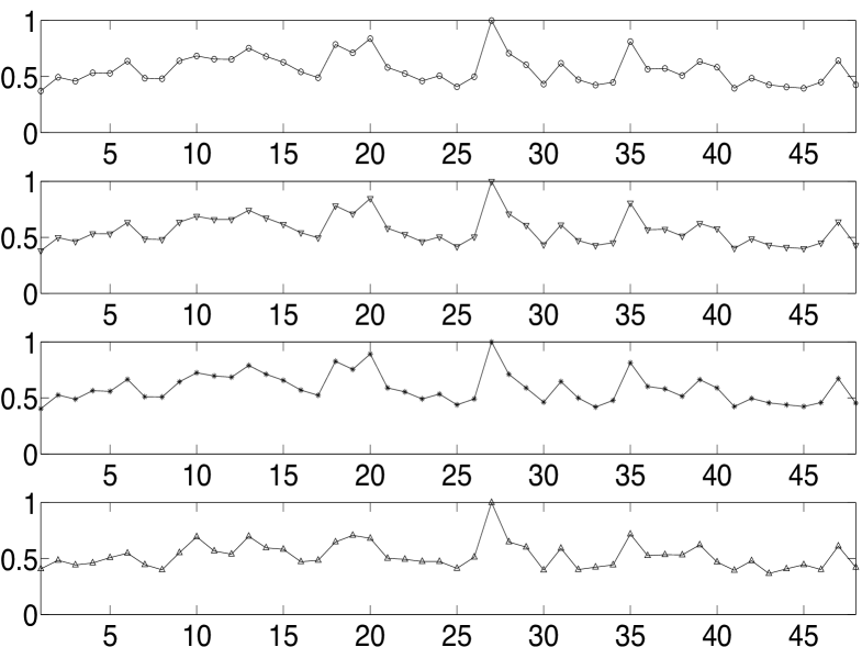
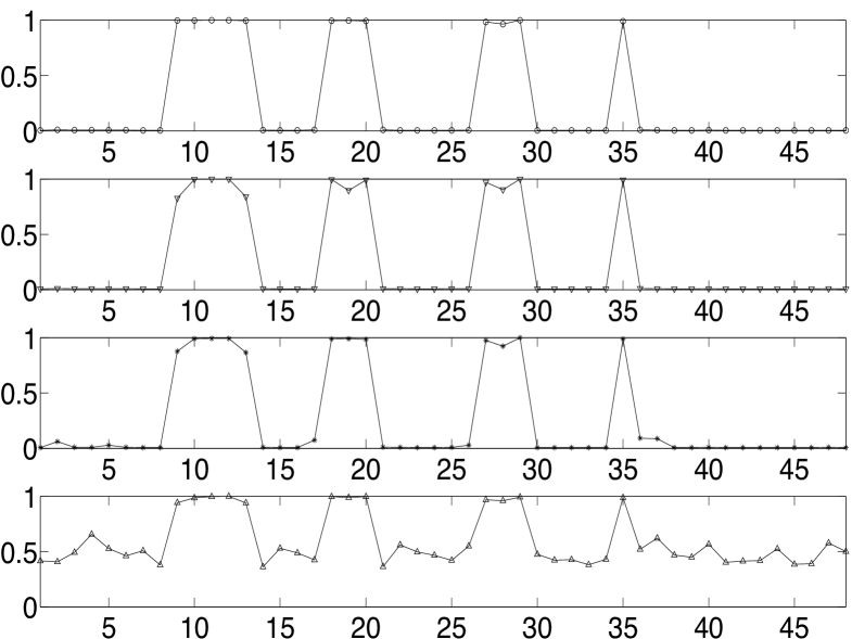
In conventional machine learning problems, complicated models are avoided fearing an over-fitted model. An over-fitted network model is usually a static network with a very large number of nodes and it tends to model the random noise or anomalies in the data rather than the underlying relationship. We evaluate the sensitivity of the weight computation algorithm or the model by analysing the change in computed weights with additive artefact noise to the data; we use weights rather than node strengths since we are analysing the model sensitivity and not evaluating a seizure focus. By adding realizations of zero mean iid noise having uniform distribution to the above analysed patient’s clinical ECoG data (taking values in ), we plot in Fig. 5(a) and Fig. 5(b) the normalised average incoming and outgoing connections for different noise variances – the average weights are normalised to have a maximum average value of for the purpose of comparison across different noise variances. The pattern in the variation of the average weights has many similar features even when the noise variance is high (fourth panel in Fig. 5(a) and Fig. 5(b)). With such a high variance of noise, we observe from Fig. 5(b) that all the nodes in the theoretically determined focus are still outgoing hubs. Similar robustness of the pattern in normalised weights were observed when the data was quantised or when the parameters (, and ) in our algorithm were varied.
Lastly, we remark that the model is flexible to changes and can be modified to work as long as the state-forgetting property is satisfied. In particular, the dynamical system at each node in (19) and inferring causality in the Algorithm in 4.1 can be made more sophisticated or changed to be based on a deeper or alternate physiological understanding of how epileptic seizures are generated.
6 Conclusions
In this paper, we have presented a modeling approach to transform data into an evolving network that has the state forgetting property or robustness to initial conditions. Although, this principle of transformation can be applied to data originating from any source, the particular evolving network model concerned an epileptic network. Although time-series can be modeled with reasonable accuracy by static networks of very large dimension such as recurrent neural networks, the individual nodes in such case have no physical significance and they do not correspond to the regions in the brain. The interconnection-strengths between the nodes were solved via a causal relationship inferred from the sustained power similarity between two nodes.
Since the model can produce a sharp reconstruction of the time-series, there is flexibility to study the interconnections in the evolving network in conjunction with the value of the time series at any time point, or over a time-interval. We have observed from modeling clinical data of an epileptic patient that certain nodes turn into outgoing hubs during the pre-ictal period and persist through the ictal period. These outgoing hubs also have a location in the brain similar to that of the clinically identified seizure onset zone (seizure focus). This hints that the (pathological) seizure causing areas in the brain could be having strong outgoing connections during seizure onset and during seizures.
Further, to quantify the influence of such outgoing hubs on the network dynamics, we have presented a result quantifying the theoretical efficacy of removal of such nodes in subsiding seizures. Of course, the result is based on data of a single patient, but then a comprehensive study of the effect of a removal of any node in an evolving network has to be backed up with a justification – since altering even a single interconnection could alter the entire network dynamics, a reliable model should show small changes in the network dynamics for small changes in the weights. In a sequel paper, we present a mathematical justification for inferring network information from a depleted network where we establish that changing the interconnections results in a continuous change in the time series whenever the evolving network is state-forgetting. Such a result is needed to justify a more detailed study of the theoretical efficacy of removal of nodes. In fact, it is possible to prove a very strong result showing that the effect of the removal of a node can be studied reliably if and only if a ‘nontrivial’ evolving network has state-forgetting property.
Acknowledgments
The author would like to thank Nishant Sinha at Nanyang Technological University for assistance in presenting plots in Section 5 and some discussions there in. The author thanks the team of the IEEG portal (https://www.ieeg.org) for providing access to the ECoG data. Access to the image(s) and/or data was supported by Award number U24NS06930 from the U.S. National Institute of Neurological Disorders and Stroke. The content of this publication/presentation is solely the responsibility of the author, and does not necessarily represent the official views of the U.S. National Institute for Neurological Disorders and Stroke or the U.S. National Institutes of Health. The author thanks an anonymous referee for pointing out several typographical errors.
References
References
- [1] Benjamin, O., Fitzgerald, T., Ashwin, P., Tsaneva-Atanasova, K., Chowdhury, F., Richardson, M. P., and Terry, J. R. (2012). A phenomenological model of seizure initiation suggests network structure may explain seizure frequency in idiopathic generalised epilepsy. J Math Neurosci, 2(1):1.
- [2] Bertram, E. H., Mangan, P., Fountain, N., Rempe, D., et al. (1998). Functional anatomy of limbic epilepsy: a proposal for central synchronization of a diffusely hyperexcitable network. Epilepsy research, 32(1):194–205.
- [3] Bonilha, L., Nesland, T., Martz, G. U., Joseph, J. E., Spampinato, M. V., Edwards, J. C., and Tabesh, A. (2012). Medial temporal lobe epilepsy is associated with neuronal fibre loss and paradoxical increase in structural connectivity of limbic structures. Journal of Neurology, Neurosurgery & Psychiatry, pages jnnp–2012.
- [4] Bragin, A., Wilson, C., and Engel, J. (2000). Chronic epileptogenesis requires development of a network of pathologically interconnected neuron clusters: a hypothesis. Epilepsia, 41(s6):S144–S152.
- [5] Breakspear, M., Roberts, J., Terry, J. R., Rodrigues, S., Mahant, N., and Robinson, P. (2006). A unifying explanation of primary generalized seizures through nonlinear brain modeling and bifurcation analysis. Cerebral Cortex, 16(9):1296–1313.
- [6] Devaney, R. L. (1989). An introduction to chaotic dynamical systems. Addison-Wesley.
- [7] Diessen, E., Diederen, S. J., Braun, K. P., Jansen, F. E., and Stam, C. J. (2013). Functional and structural brain networks in epilepsy: what have we learned? Epilepsia, 54(11):1855–1865.
- [8] Elaydi, S. (2005). An introduction to difference equations. Springer Science & Business Media.
- [9] FitzHugh, R. (1969). Mathematical models of excitation and propagation in nerve. In Biological engineering, pages 1–85. McGraw-Hill, New York.
- [10] Furi, M. and Martelli, M. (1991). On the mean value theorem, inequality, and inclusion. American Mathematical Monthly, pages 840–846.
- [11] Hutchings, F., Han, C. E., Keller, S. S., Weber, B., Taylor, P. N., and Kaiser, M. (2015). Predicting surgery targets in temporal lobe epilepsy through structural connectome based simulations. PLoS Comput Biol, 11(12):e1004642.
- [12] Jaeger, H. (2001). The “echo state” approach to analysing and training recurrent neural networks-with an erratum note. Bonn, Germany: German National Research Center for Information Technology GMD Technical Report, 148:34.
- [13] Jansen, B. H. and Rit, V. G. (1995). Electroencephalogram and visual evoked potential generation in a mathematical model of coupled cortical columns. Biological cybernetics, 73(4):357–366.
- [14] Jirsa, V. K., Stacey, W. C., Quilichini, P. P., Ivanov, A. I., and Bernard, C. (2014). On the nature of seizure dynamics. Brain, 137(8):2210–2230.
- [15] Kalitzin, S. N., Velis, D. N., and da Silva, F. H. L. (2010). Stimulation-based anticipation and control of state transitions in the epileptic brain. Epilepsy & Behavior, 17(3):310–323.
- [16] Khosravani, H., Mehrotra, N., Rigby, M., Hader, W. J., Pinnegar, C. R., Pillay, N., Wiebe, S., and Federico, P. (2009). Spatial localization and time-dependant changes of electrographic high frequency oscillations in human temporal lobe epilepsy. Epilepsia, 50(4):605–616.
- [17] Kloeden, P., Pötzsche, C., and Rasmussen, M. (2013). Discrete-time nonautonomous dynamical systems. In Stability and bifurcation theory for non-autonomous differential equations, pages 35–102. Springer.
- [18] Kloeden, P. E. and Rasmussen, M. (2011). Nonautonomous dynamical systems. Number 176. American Mathematical Soc., Providence.
- [19] Kramer, M. A. and Cash, S. S. (2012). Epilepsy as a disorder of cortical network organization. The Neuroscientist, 18(4):360–372.
- [20] Lemieux, L., Daunizeau, J., and Walker, M. C. (2011). Concepts of connectivity and human epileptic activity. Frontiers in systems neuroscience, 5:1–13.
- [21] Maass, W., Natschläger, T., and Markram, H. (2002). Real-time computing without stable states: A new framework for neural computation based on perturbations. Neural computation, 14(11):2531–2560.
- [22] Manjunath, G. and Jaeger, H. (2013). Echo state property linked to an input: Exploring a fundamental characteristic of recurrent neural networks. Neural computation, 25(3):671–696.
- [23] Manjunath, G. and Jaeger, H. (2014). The dynamics of random difference equations is remodeled by closed relations. SIAM Journal on Mathematical Analysis, 46(1):459–483.
- [24] Marten, F., Rodrigues, S., Suffczynski, P., Richardson, M. P., and Terry, J. R. (2009). Derivation and analysis of an ordinary differential equation mean-field model for studying clinically recorded epilepsy dynamics. Physical Review E, 79(2):021911.
- [25] Morgan, R. J. and Soltesz, I. (2008). Nonrandom connectivity of the epileptic dentate gyrus predicts a major role for neuronal hubs in seizures. Proceedings of the National Academy of Sciences, 105(16):6179–6184.
- [26] Ngugi, A. K., Bottomley, C., Kleinschmidt, I., Sander, J. W., and Newton, C. R. (2010). Estimation of the burden of active and life-time epilepsy: a meta-analytic approach. Epilepsia, 51(5):883–890.
- [27] Richardson, M. P. (2012). Large scale brain models of epilepsy: dynamics meets connectomics. Journal of Neurology, Neurosurgery & Psychiatry, 83(12):1238–1248.
- [28] Robinson, P., Rennie, C., and Rowe, D. (2002). Dynamics of large-scale brain activity in normal arousal states and epileptic seizures. Physical Review E, 65(4):041924.
- [29] Rocsoreanu, C., Georgescu, A., and Giurgiteanu, N. (2012). The FitzHugh-Nagumo model: bifurcation and dynamics, volume 10. Springer Science & Business Media.
- [30] Schmidt, H., Petkov, G., Richardson, M. P., and Terry, J. R. (2014). Dynamics on networks: the role of local dynamics and global networks on the emergence of hypersynchronous neural activity. PLoS Comput Biol, 10(11):e1003947.
- [31] Silva, F. H., Blanes, W., Kalitzin, S. N., Parra, J., Suffczynski, P., and Velis, D. N. (2003). Dynamical diseases of brain systems: different routes to epileptic seizures. Biomedical Engineering, IEEE Transactions on, 50(5):540–548.
- [32] Spencer, S. S. (2002). Neural networks in human epilepsy: evidence of and implications for treatment. Epilepsia, 43(3):219–227.
- [33] Steil, J. J. (2004). Backpropagation-decorrelation: online recurrent learning with o (n) complexity. In Neural Networks, 2004. Proceedings. 2004 IEEE International Joint Conference on, volume 2, pages 843–848. IEEE.
- [34] Suffczynski, P., Kalitzin, S., and Da Silva, F. L. (2004). Dynamics of non-convulsive epileptic phenomena modeled by a bistable neuronal network. Neuroscience, 126(2):467–484.
- [35] Taylor, P. N., Goodfellow, M., Wang, Y., and Baier, G. (2013). Towards a large-scale model of patient-specific epileptic spike-wave discharges. Biological cybernetics, 107(1):83–94.
- [36] Terry, J. R., Benjamin, O., and Richardson, M. P. (2012). Seizure generation: the role of nodes and networks. Epilepsia, 53(9):e166–e169.
- [37] Wendling, F., Bartolomei, F., Bellanger, J., and Chauvel, P. (2002). Epileptic fast activity can be explained by a model of impaired gabaergic dendritic inhibition. European Journal of Neuroscience, 15(9):1499–1508.
- [38] Wendling, F., Hernandez, A., Bellanger, J.-J., Chauvel, P., and Bartolomei, F. (2005). Interictal to ictal transition in human temporal lobe epilepsy: insights from a computational model of intracerebral eeg. Journal of Clinical Neurophysiology, 22(5):343.
Appendix A Appendix: Autonomous vs. Nonautonomous Dynamics
When interconnections change with time in a network of dynamical systems, the overall dynamics of the entire network is nonautonomous – autonomous dynamics is rendered when systems evolve according to a rule fixed for all time, and when it is not fixed (here, due to the time-varying interconnections), nonautonomous dynamics emerges (see Section 2 for definitions). The evolution of an autonomous system depends on only the initial condition presented to it, whereas in a nonautonomous system the evolution depends both on the initial condition and the time at which it is presented. The evolution of an autonomous system in discrete-time can be described by an update equation , where is a function governing the rule for evolution. The evolution of a nonautonomous system can be described by an update equation , where a family of maps govern the rule of evolution.
We explain the advantage of considering a nonautonomous model. Consider a two-dimensional autonomous dynamical system which updates its dynamics according to the rule ( and are any functions whose domain and range are and ) to generate a -dimensional time series . Suppose in reality, only the first coordinate or dimension of the time series, i.e, is observable. Then, in general it is not possible to model the time-series as the dynamics of a one-dimensional dynamical system, in other words it is not possible to find a function (map) so that holds for all since inherently depends on . However, it is possible to find a nonautonomous system, i.e., a family of maps so that . In general, whenever we are unable to completely observe all the variables from a dynamical system (including nonautonomous systems) it is possible to synthesise a nonautonomous system that models the observed variables. In real world systems, the non-autonomous system can account for obfuscated factors such as the unfeasibility of observing all variables, exogenous influence etc. by subsuming their net-effect by a collection or family of maps that vary with time.
Appendix B Appendix: Formal Definition of State Forgetting Property
Mathematically, viewing an evolving network as a static network being acted upon by an exogenous stimulus that influences the network connections at each time step gives us the advantage of employing the formal framework of the echo-state static networks theory in machine learning [12, 22]. We recall some notions [12, 22] and adapt to our setup. We begin now with a formal description.
Here, and throughout, only the Euclidean distance is employed as a metric/distance on any two elements of . Also represents a nondegenerate compact interval of , and denotes the -times product .
Following [22, 23] and several others (e.g., [8, 17, 18]), we define a discrete-time nonautonomous system on a metric space as a sequence of maps , where each is a continuous map. Any sequence that satisfies for all is called an entire-solution of . For the discussion in this paper it is sufficient to consider an evolving network with each of the nodes having a one-dimensional dynamical system on an interval , i.e., for an isolated node, there is some function mapping to as it is an autonomous system. We formally define an evolving network below:
Definition B.1
Let be a compact interval of , and let be an integer. Suppose a function has a real-valued matrix , and a value in as its arguments and maps it to a value in for each , i.e., is such that
-
(i)
is continuous and
-
(ii)
is defined by a set of (continuous) coordinate maps such that , where represents the row of a matrix , and the component of ; here generates the node dynamics at the node,
then such a map is called a family of evolving network. If in particular, a bi-infinite sequence of matrices is fixed, then the sequence of mappings is referred to as an evolving network.
Clearly, any evolving network is also a nonautonomous system on if we set for all . We call the connectivity weight matrix or just the weight matrix.
We next define the state-forgetting property of a family of evolving networks and also for a particular evolving network.
Definition B.2
Let be a family of evolving networks. If for each choice of , the evolving network has exactly one entire-solution, then the family of evolving networks is said to be state-forgetting. In particular, for any fixed , the corresponding evolving network (or the nonautonomous system) is said to be state-forgetting if it has exactly one entire-solution.
Appendix C Appendix: Proof of State Forgetting Property
We first recall some preliminaries and known results that help us in presenting the proof of Theorem 3.3.1.
It is convenient to have the following alternate representation of a nonautonomous system. Let the collection of all integer tuples so that , i.e., . Given a nonautonomous system on , it is convenient (see [22]) to denote the nonautonomous system through a function called a process on that satisfies: and We say has the state-forgetting property if has the state-forgetting property.
The following Lemma is reproduced from [22, Lemma 2.2].
Lemma C.1
Let be a process on a compact metric space metrized by . Suppose that, for all , there exists a sequence of positive reals converging to such that for all and for all . Then has the state-forgetting property, i.e., there is exactly one entire solution of the process .
The essence of the following result is that if has the state-forgetting property then all initial conditions converge to the unique entire-solution in Proposition C.1. For a detailed explanation see [23] and references therein.
Proposition C.1
Let be a process on a compact metric space metrized by . Suppose is the unique entire-solution of , then for all and .
We repeatedly use the following standard inequalities involving the infinity norm and spectral norm: and for all ; when , .
A generalization of the mean-value theorem in one-dimensional calculus to higher dimensions results in the following mean-value inequality (e.g., [10]). This result can be stated as: if is a -function where is an open subset of then for any
| (C-29) |
where is the -norm, and is the induced norm of the Jacobian of at the point .
To simplify the notations in the proof of Theorem 3.3.1, whenever , we adopt the notation
and
, where and are column vectors and the superscript represents the transpose of the vector .
Proof of Theorem 3.3.1. Fix a that satisfies (23) for all and . Let be defined by , where is as in (21). Since fixing a or a ( related to by (21)) amounts to fixing an evolving network, we have fixed a nonautonomous system.
In the notion of a process, the evolving network update obtained by varying from to in (23) can be represented at time by
where , and
, with as the column vector . Since the function in (22), ensures , we have
| (C-30) |
Since the choice of was made arbitrarily, if we show that has exactly one-entire solution then we would have shown that the evolving network is state-forgetting by Definition B.2. Since is a process on , a compact subset of , we make use of Lemma C.1 to show has exactly one-entire solution. We employ the metric induced by the norm for getting an inequality of the form in Lemma C.1.
Let be any real number in . We first aim to show that there exists a (that depends on ) such that for all , the following inequality is satisfied.
| (C-31) |
We next proceed to prove for all . Recall that . We first consider the first term on the right hand side, i.e., and prove an upper bound for using the mean value theorem.
Since is differentiable and has a continuous derivative, by applying the mean value theorem on the domain we infer:
| (C-32) |
by hypotheses, and . If , it is straightforward to deduce the following equivalent statements: for all for all (since ) for all for all since the derivative .
Since is continuous, for all implies for all . Using this in (C-32), it follows that
| (C-33) |
Now,
| (C-34) | |||||
Let be such that . Since , the Jacobian evaluated at is a diagonal matrix and the diagonal element of this matrix is found to be
| (C-35) |
The following deductions give an upper bound for :
| (C-36) | |||||