Exact--Relation Graphs
Abstract
Pairwise compatibility graphs (PCGs) with non-negative integer edge weights recently have been used to describe rare evolutionary events and scenarios with horizontal gene transfer. Here we consider the case that vertices are separated by exactly two discrete events: Given a tree with leaf set and edge-weights , the non-negative integer pairwise compatibility graph has vertex set and is an edge whenever the sum of the non-negative integer weights along the unique path from to in equals . A graph has a representation as if and only if its point-determining quotient is a block graph, where two vertices are in relation if they have the same neighborhood in . If is of this type, a labeled tree explaining can be constructed efficiently. In addition, we consider an oriented version of this class of graphs.
keywords:
Pairwise compatibility graphs , edge-labeled trees , thin graphs , block graphs , oriented graphsMSC:
05C75 , 05C05 , 92B101 Introduction
Consider a tree with leaf set and a non-negative edge-weight function . Denote by the unique path between and in . The canonical distance function is then defined by
| (1) |
This definition is the starting point for mathematical phylogenetics, which is centered around finite additive metric spaces and their generalizations [1, 2]. It also serves as a basis for defining a large class of graphs that in the recent past has received considerable attention. The pairwise compatibility graphs has vertex set and edges
| (2) |
Originally introduced in the context of phylogenetics [3], they have received considerable interest in the last years, see [4, 5] and the references therein, as well as [6, 7, 8]. A further generalization of “multi-interval” PCGs in explored in [9]. In the setting of PCGs and most phylogenetic applications one usually stipulates that , measuring e.g. the time between two distinct events associated with adjacent vertices of . A class of graphs that is conceptually closely are the exact -leaf powers [10], for which for all edges of and .
In an alternative interpretation, models the number of discrete evolutionary events along an edge of of . This is of interest in particular in the context of so-called rare genomic changes such as the gene or loss of a particular gene of gene family or a particular genomic rearragement [11]. Some of these convey phylogenetic information that is (nearly) free of homoplasy, i.e., the independent occurrance in independent lineages. Examples of such rare events are the emergence of novel microRNA families [12] or rearrangements of the genomic gene order [13]. Since such events are very unlikely to have occurred more than once in the same manner, they identify phylogenetic groupings that share such an innovation with very little ambiguity. This provides information to resolve also parts the phylogenetic tree where classical, sequence-based methods fail [14]. In this context it is necessary to allow because the events of interest are by definition so rare that not all taxa will be distinguished by them. In the same vein it important that events are discrete and hence an integer-valued weight function . Both conditions on cause subtle but important differences in comparison with the usual definition of PCGs that requires non-zero edge length but otherwise allows arbitrary real values. We will denote these “non-negative integer pairwise compatibility graph” by nniPCG to distinguish them from the better studied class of PCGs with non-zero real-valued edge weights .
The special case in which two leaves and of are separated by a single event, corresponding to graphs of the form , was explored in [15] as a model of rare events in evolution. It turns out that this graph class coincides with the forests. The graphs requiring at least one event along the path between two leaves also have a very simple structure: they are exactly the complete multipartite graphs [16].
Considering a rooted tree instead of an unrooted tree , it is natural to consider the digraphs with edges whenever a certain number of events occured between the last common ancestor and . This construction appears naturally in the context of horizontal gene transfer (HGT), where one asks whether and are separated by at least one HGT event111HGT refer to the import of gene from an unrelated species e.g. through an infection, ingestion, acquisition via a plasmid. This gives rise to the class of Fitch graphs [17], which form a subclass of di-cographs introduced by [18]. Their underlying undirected graphs are exactly the , i.e., the complete multipartite graphs.
A related construction requires a certain number of events between and and excludes all events between and . This class of graphs appears naturally when events are directed, i.e., when it is (in general) no possible to revert the effect of an operation in a single step. Probably the best studied type of single genomic events of this type are so-called Tandem-Duplication-Random-Loss events, during which a genomic interval is duplicated and then one of the two copies of each gene is lost at random [19]. The antisymmetric digraphs obtained by single events are characterized in [15].
Our interest in the graphs for general also stems from rare-event phylogenetic data. Since we assume an underlying tree, the distance matrix is additive and its entries are small non-negative integers. The fact that all edge lengths are also integers of course imposes additional constraints. As demonstrated e.g. in the context of orthology assignment (a related problem with vertex labeled trees for which the corresponding graphs turn out to be cographs), graph editing can be employed to correct empirically estimated input graphs [20]. This approach requires, however, that constraint on the graphs that can appear are known. In the case of rare-event phylogenetics, we know that the graph with edge set must be a . In the rare-event scenario, the number of pairs of nodes with will quickly decrease with , so that the empirical input graphs will have few edges for larger values of and thus rarely reveal obstructions. Hence only small value of are of practical value for detecting measurement errors in the data. Since the are forests, the corresponding graph editing problem amounts to identifying spanning forests, and possible false positive events are edges in cycles. False negatives are not detectable for since there are no non-tree graphs that would become trees by inserting edges. They could be detected, however, as missing edges in the empirical graph for compared to the most similar member of . In this contribution, therefore, we are interested in the characterization of the graphs , in which edges correspond to exactly two events between two leaves. This graph class is very different from the exact-2-leaf power graphs, which are known to coincide with the disjoint unions of cliques [21, 10]. In contrast, we shall see below that e.g. every path also has a representation as .
This contribution is organized as follows: We first consider a few general properties of the slightly more general exactly--relation before investigating for some small graphs and simple graph families whether they can be respresented with respect to the exactly--relation on the leaf set of some tree. Here, we consider the case that , i.e., that all leaves are separated by at least one event, and then relax this constraint and characterize the entire graph class for non-negative, integer . Our main result is that these graphs are those whose quotient with respect to the false twin (R-thinness) relation is a block graph. We then consider the oriented version of the problem and give characterization in terms of forbidden subgraphs.
2 Simple Properties of the Exactly--Relation
We shall see that the restriction to integer edge weights on the one hand, and the admission of zero-weights on the other hand, make the graphs quite different from the exact--leaf power graphs studies systematically in [10]. While it is true that every with non-negative real weigths and bounds and also has a representation as with integer weights and bounds [22, Lemma 2], the restriction to integer weights clearly affects the definition of graph classes. For instance, the PCG class with rational weights and bounds contains the for all . Throughout this contribution we use a notation that is inspired by related work in mathematical phylogenetics.
Definition 1.
Let be an unrooted tree with leaf set and edge-labeling
function . For we consider the
exactly--relation defined by if the
(unique) path from to in satisfies
.
Furthermore, we say
explains a graph (with respect to the
exactly--relation) if if and only if .
We consider unrooted instead of rooted tree since the distances and thus the exactly--relation contains no information on position of root. In fact, it is well known [23, 24] that a metric of the form (1) uniquely defines an unrooted tree. Therefore, one can only hope to reconstruct the unrooted tree .
Definition 2.
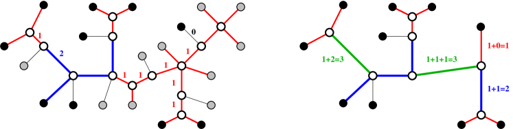
The edge-labeled tree displays the edge labeled tree if can be obtained from by first removing every edge and vertex from that is not contained in a path connecting two leaves of , and then contracting every path in the remainder of that has only interior vertices of degree by a single edge in with label .
In particular, therefore it is sufficient to consider phylogenetic trees, that is, trees in which every interior node has degree at least . Fig. 1 gives an example. A simple, but important consequence of Definition 1 is the following
Lemma 3.
If displays , explains
and explains .
Then
, the subgraph of induced by .
Proof.
If displays then for all , and thus we conclude that for all , we have if and only if , i.e., is the subgraph of induced by . ∎
It follows that “being explained with respect to the exactly--relation” is a hereditary graph property for all .
We also note the following immediate consequence of the definition.
Lemma 4.
If explains with respect to , then explains with respect to .
Lemma 5.
Let be a graph with connected components , . Then there is an edge-labeled tree explaining with respect to if and only if there are edge labeled trees explaining for all .
Proof.
The condition is necessary because of heredity. In order to see sufficiency, we can construct from the disjoint union of the in the following way: first we arrange them as an arbitrary tree . Then we replace each by with the two edges and labeled such that . Now choose for each tree an arbitrary inner vertex in and the unique vertex if . Finally, we connect and by an edge with if and only if and are adjacent in . To verify that indeed explains we observe: (i) If and are leafs from different connected components of , they are located in different subtrees and thus the path connecting them contains one of the edges label , thus and are not in relation . ∎
It is therefore sufficient to consider connected graphs.
Definition 6.
An edge-labeled graph is canonical if is phylogenetic and for all interior edges.
Lemma 7.
Let be the edge labeled tree obtained from by (1) replacing every path in whose interior vertices have degree by a single edge in with label and (2) contracting every interior edge with . The tree is uniquely defined, canonical, and explains the same graph as .
Proof.
The maximal paths with interior vertices of degree in are disjoint and thus can be treated independently. By construction, any such path can also be stepwisely replaced by edges, eventually arriving at the same edge weight for the single edge that remains. Given , the resulting tree is therefore unique and contains no vertex of degree . It is therefore phylogenetic. Since an interior edge with label does not contribute the total weight of any path that runs through it, it can be contracted without changing the total path weights between leaves. Thus and explain the same graph. ∎
Consider two leaves in an edge-labeled tree such that , i.e., , and another leaf . The triangle inequalities and implies . Thus and have the same neighbors in graph explained by , i.e., .
Definition 8.
Let be a graph. For each denote by the neighbors of . Two vertices and are false twins, , if .
In contrast, true twins, which play no role here, satisfy . By definition, false twins are non-adjacent, while true twins are always adjacent [25].
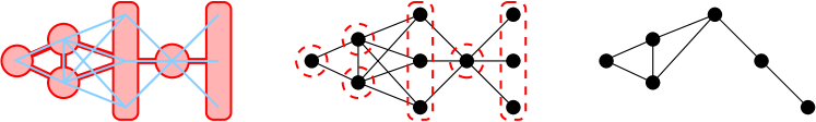
The false twin (R-thinness) relation has been well studied in the literature, in particular in the context of graph products [26]. It is well known that is an equivalence relation, see e.g. [26, sect. 8.2]. Its equivalence classes, which we denote by , , are totally disconnected in because, by definition, . Denote by be the subgraph of induced by one arbitrarily chosen representative of each false twin class. Since for any and we have if and only for all and all we observe that and the quotient graph are isomorphic. An illustration is given in Fig. 2.
Lemma 9.
Let be a canonical tree explaining a connected graph with respect to , and let be a set of sibling leaves attached to the same parent with for all . Then is contained in a false twin class for the graph explained by with respect to for all .
Proof.
Consider a node . Then the total weight of the path between and every is the same. Furthermore, the total path weight between any two vertices in is , i.e., there is no edge between and . Thus , i.e., for all . ∎
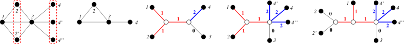
A graph is called R-thin [27], point determining graph [28] or mating graph [29] if is discrete, i.e., every false twin class consists of only a single point. Clearly, is R-thin. R-thin graphs have also been studied from the point of view of combinatorial enumeration [30, 31]. Algorithms for prime-factorization of graphs, furthermore, often operate on , since R-thinness ensures uniqueness of the factorization and allows for highly efficient algorithms [27, 32, 26]. Below we show that it also suffices to consider , i.e., R-thin graphs, in our setting. Indeed, a simple consequence of Lemma 9 is
Corollary 10.
If is R-thin and is a canonical tree explaining with respect to , then is discrete.
For an illustrative example see Fig. 3.
Theorem 11.
can be explained w.r.t. if and only can explained w.r.t. . If is a canonical tree explaining , then a canonical tree explaining is obtained by Algorithm 1.
Proof.
Since can be explained and is an induced subgraph of , can be explained w.r.t. to by a tree that we denote by . Let be the representative of the false twin class of , and let . Insert into are a sibling of and set . Then and have the same total path weights to all other vertices. This remains true if each leaf in is replaced in this manner by the set of sibling vertices with . Since no two vertices in are adjacent we require that , i.e., . If this conditions is satisfied, then explains with respect to .
If , Alg. 1 inserts an extra vertex adjacent to with . Since we assumed that was canonical, has at least two more neighbors, i.e., the resulting tree is again canonical. Since is attached with edge weights we conclude that (i) the total path weight between and is and (ii) for all , i.e., and are not adjacent in the graph explained by . Hence and have the same neighbors and thus belong the same false twin class of . Since the total path weights between all representatives of false twin classes are preserved by this construction, indeed explains with respect to . We note, finally, that is again canonical because has at least three neighbors (the parent and at least members of ), and all interior edges the resulting tree have non-zero labels as long as was canonical. ∎
From here on we will therefore assume the is canonical, i.e., it has non-zero labels for all inner edges of . It is important to note, however, that we still need to consider zero weights on the edges incident with leaves. For instance, it not difficult to check that the graph in Fig. 3, i.e., , cannot be explained by a tree with only non-zero edge weights.
3 Graphs Explained w.r.t.
We will first consider the special case of edge labelings with discrete . In this case every interior vertex of is incident with at most one zero-weight edge.
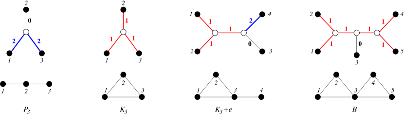
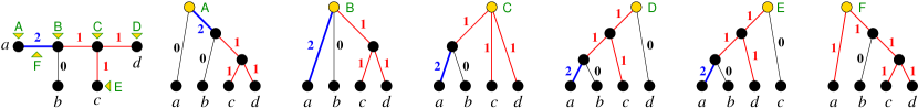
The trivial cases and are explained by the trees and with label at the unique edge , respectively. For there is only a single phylogenetic tree, the star with three leaves and two connected graphs, , and , see Fig. 4. We denote the edges from the center to leaf by , . Fig. 4 also shows that class of graphs explained w.r.t. is much larger than the exact-2-leaf powers graphs, which comprise only the disjoint unions of cliques [21, 10].
Lemma 12.
There are unique labelings and of the
tree with discrete that explain the graphs
and , respectively:
and ;
;
Proof.
contains three paths on length two.
Adopting the notation of Fig. 4 for both cases and
we need and
. Therefore .
Explicitly enumerating the three cases yields:
implies and thus ,
in which case , contradicting the fact is discrete.
implies , and thus
.
implies and thus ,
whence .
∎
Lemma 13.
The path on four vertices is explained only be the tree with labels and .
Proof.
First we observe that the path on four vertices cannot be explained by any labeling of a . This leaves the fully resolved tree on four vertices. Its interior edge cannot be labeled . First consider . It cannot contain an with all three edges labeled since this would induce a triangle, i.e., at most one neighbor of , say , is attached by a 1-edge. The other neighbor of , call it , then must be attached by a -edge, since otherwise is isolated. In order for not to be isolated, also must have a neighbor, that is connected via a -edge, say . The same argument implies the the remaining leaf must be connected to with . This tree, however, explains the non-connected graph . Thus . Connectedness implies that at least one of the leaves attached to and must be labeled , say , and thus and are adjacent in . It remains to consider the possible coloring for the remaining to edges and . If then is isolated for all choices of . An analogous statement is true for . For we obtain . If and we obtain . The same is true for and . Thus the only remaining choice is . It indeed explains the path , see Fig. 5. ∎
The fact that is the only “exact-2-leaf root” of , i.e., the only tree with unit edge weights that explains is shown in [10, Lemma 2]. It is not difficult to see that there is also no other choice of non-negative integer labels on that explains :
Lemma 14.
The complete graph is explained with respect to by the star with the unique labeling function for all .
Proof.
Is is easy to check that this construction explains for all . The trivial cases and are explained in the text. is only explained by with all edges labeled . Since the start displays corresponding to every subgraph, all edges of must be labeled by . ∎
We note for later reference that the uniqueness results in Lemmas 13 and 14 do not require the precondition that is discrete. This observation will be important in the following section.
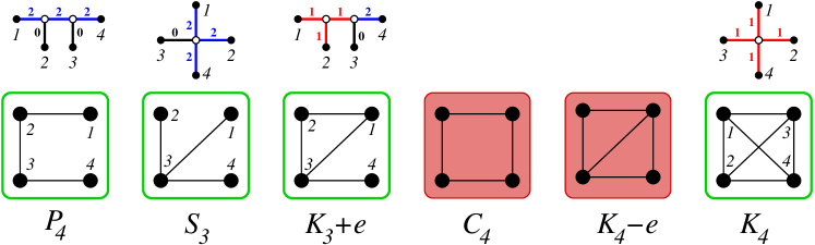
Lemma 15.
There is no edge-labeled tree with discrete that explains the graphs and with respect to . The graph is explained by a unique edge-labeled tree.
Proof.
There are two topologically distinct trees for , the star and tree with a single interior split. First consider the star . In order to explain or three of the four edges must be labeled (corresponding to the induced . Depending on whether or , the fourth vertex is either connected to all or none of the three other vertices. In order explain , there must be two edges with and one with corresponding to an induced . The remaining edge then must have . But then , contradicting that is discrete.
Now consider the tree, which can be obtained from by subviding one of the edges and attaching an extra leaf to the subdividing vertex. Denote by the (unique) inner edge of . Consider and as shown in Fig. 5. Then we must have . If we recover the situation of , since the inner edge does not contribute to . On the other hand, if If , then and cannot be connected with or , contradicting the existence of as induced subgraph. Thus . Then . By assumption, since otherwise . If , the is an isolated vertex in . If , then while is not in relation to either or . Thus . The corresponding edge labeled tree is shown in Fig. 4. Since we have already considered all cases, cannot be explained with respect to .
Finally, consider and suppose that contains as induced subgraph. There are two cases: If then connectedness of implies that , contradicting that is discrete. In the alternative case we can assume, w.l.o.g., that and . Furthermore, in order to explain we must have . If both . Then and yields , for we obtain . In the remaining case we can choose and . Now contradicts discreteness of , yields the edgeless graph. For we obtain . Thus cannot be explained by with respect to by a labeling with discrete . ∎
The fact that is a forbidden subgraph implies that two cliques in cannot be “glued together” by a single common edges. It is possible, however, for cliques to touch in a cut vertex as shown by the example of the bowtie graph , which is obtained by gluing together two triangles at a common vertex, see Fig. 4.
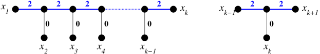
Graphs that can be represented as pairwise compatibility graphs of caterpillars have received special attention in the literature [5, 33, 34, 35]. It is not difficult to see that the path , can represented by a caterpillar in several settings. These results cannot be directly applied in our setting, however. Any two leaves and attached to two distinct inner vertices of a caterpillar are separated by at least three edges an thus cannot be in relation if we assume strictly positive integer weights. It follows immediately that is not an exact-2-leaf power of a caterpillar and that cannot be explained by caterpillar unless zero-weights are allowed. An explicit construction in [15] shows that is explained by a caterpillar with edge weights in with respect to exactly-1-relation . Lemma 4 implies that we can use the same construction to explain by a caterpillar with edge weights in , see Fig. 6. It will be important later on that this construction is indeed unique:
Lemma 16.
The path has as its unique explaining tree the caterpillar with all inner edges and the edges connecting to the end-points of labeled and all edges connecting to inner vertices of labeled .
Proof.
We first recall that the tree explaining is unique by Lemma 13. Now assume that for , the tree explaining is unique and thus a caterpillar. Any tree explaining therefore must display , i.e., is obtained from by subdiving one edge and attaching leaf and edge to the new vertex, or by attaching and to an inner vertex of . One easily checks that the latter yields a branched tree or a disconnected graph. The same is true is any other edge except and , the edges adjacent to the leaves or are subdivided. In the latter case, cannot be adjacent to . In the remaining case, the edge with which is attached is subdivided into an interior part and the part incident with . Since the interior part cannot carry a zero label, we must have , , and . Thus the caterpillar of Fig. 6 is indeed the only choice. We emphasize that this observation remains true even is is not assumed to be discrete. ∎
Lemma 17.
The simple cycles , cannot be explained with respect to irrespective of whether is discrete or not.
Proof.
Every cycle contains a path with one vertex less as an induced subgraph. From Lemma 16 we known that has a unique explanation by a caterpillar for all . Thus any tree explaining thus must display caterpillar and thus is obtained from by either attaching and to inner vertex of or by subdiving an edge and attaching and to the newly inserted vertex. As argued above, attachment to an inner vertex or subdivision of an edge other than or leads to a branched tree or a disconnected graph. If is inserted by subdivision of , then cannot be adjacent to and subdivision of precludes adjacency of and for . Thus the catapillar tree cannot be extented to tree that explains for any . Note that this argument did not make the assumption that is discrete. ∎
Let us now turn to the general case. We first note that all graphs explained w.r.t. with discrete are chordal, i.e., every cycle of length greater than three has a chord. Even more stringently, every cycle of length corresponds to a clique in because the , i.e., the 4-cycle with a chord, is also a forbidden induced subgraph. We note that there is ample literature on the relationship of chordal graphs and PCGs, see e.g. [4, 5]. Due to the differences in the edge weight functions, it is not immediately pertinent to our discussion, however.
Lemma 18.
If can be explained by the exact--relation with discrete and contains a Hamiltonian cycle, then is a complete graph.
Proof.
The assertion is trivially true for and holds for because and , the only Hamiltonian graphs on 4 vertices except are forbidden induced subgraphs. Now suppose the statement is true for for all and consider a graph with vertices. Since is chordal, there is in particular a planar triangulation of that is a subgraph of and thus there are three consecutive vertices along such that is a also an edge in . Thus is Hamiltonian. As an induced subgraph of it can be explained by the exact--relation and thus is a complete graph by the induction hypothesis. Thus is triangle in and is a cycle of length in . Since and cannot appear as induced subgraphs of , must for a clique in , and hence the edge for all . Thus is a complete graph. ∎
Lemma 19.
A graph with at least three vertices that can be explained by the exact-2-relation with discrete is complete if and only if it is 2-connected.
Proof.
If is Hamiltonian, it is in particular also 2-connected. Now consider the case that is 2-connected but not Hamiltonian. Let be a cycle of maximal length in and let be a vertex not in . Then there is a cycle in that contains and at least two distinct vertices of since otherwise one of the vertices of would be a cut vertex of , contradicting 2-connectedness. Starting from , let and be first and last vertex of encountered along . By Lemma 18, is a complete graph, and hence there is a another Hamiltonian cycle on so that and are consecutive along . Thus the cycle obtained traversing from to and then following from through back to is a cycle that is strictly longer than , contradicting maximality. Thus is Hamiltonian, and hence complete. ∎
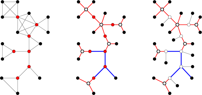
A graph is a block graph [36] if each of its biconnected components is a clique. Lemma 19 thus implies that every graph that can be explained with respect to the exact--relations with discrete is a block graph (see Thm. 21 below for a formal proof). Algorithm 2 (illustrated in Figure 7) explicitly constructs an edge-labeled tree that explains a given block graph.
Lemma 20.
Algorithm 2 transforms any connected block-graph into an edge-labeled tree that explains with respect to the exactly--relation with discrete .
Proof.
The output of Alg. 2 contains no cycles since all cycles in the input are contained within a block and each block is replaced by a star. Furthermore, the replacement of a clique by a star with vertices preserves connectedness, hence has been transformed into a tree at this stage. Every vertex of a clique , with this is not also contained in another block is now a leaf; all other nodes of are marked red. Every vertex in an original block is either a leaf or marked “red”. By construction, every “red” vertex has degree at least and hence is not a leaf. The final operation adds a leaf to each “red” vertex. Together with the renaming of the vertices, thus, every vertex of the input graph is now a leaf in .
Now consider the labeling. First suppose that and are non-adjacent in the input , that is, there is a least one cut-vertex, say , between them in . The construction of ensures that the unique path from to in runs through a vertex that as its neighbor. If the path from to in ran through an edge in a triangle, it passes through the corresponding star and hence contains two edges labeled . Otherwise it runs through an unaltered -block of , which is labeled . In each case, therefore, . Now suppose that and are adjacent in . First suppose is contained in a triangle of . If neither nor was marked “red” they are both adjacent to the center of a star with edges labeled . If was a cut vertex, i.e., marked “red”, it appears a leaf adjacent to a vertex that in turn is adjacent to ; furthermore and . Analogous reasoning applied if was a cut vertex of . In all cases, thus . If the edge is not contained in a triangle, then it is labeled . If or are cut vertices, then the unique path from to is , , or , with and a label for the remaining edge. Hence, . In summary if and only and are adjacent in . Thus is explained by with respect to the exactly--relation. ∎
Theorem 21.
A graph can be explained by an edge-labeled tree with respect to the exact--relation with discrete if and only if it is a block graph.
Proof.
Suppose can be explained w.r.t. with discrete . If is 2-connected, it is a clique by Lemma 19 and therefore also a block graph. Otherwise, we note that every 2-connected component of is induced subgraph of and thus, by Lemma 3, can be explained w.r.t. . By Lemma 19 every 2-connected component of therefore must be a clique, i.e., is a block graph.
The main result of this section is now obtained as
Corollary 22.
A graph is explained by if and only if is a block graph.
Proof.
In the remainder of this section we consider the ambiguities in the construction of trees explaining block graphs. We start by characterizing contractible edges:
Lemma 23.
Suppose is obtained from a phylogenetic tree by contracting the edge in and setting for all and suppose that is connected. Then if and only if is an interior edge of and .
Proof.
We have already noted the contracting an inner -edge does not change the graph. By definition, leaf-edges cannot be contracted, since the vertices of correspond to the leaves of . Connectedness of implies that there is a pair of vertices whose connecting path runs through and whose distance . The contraction of only leaves this distance unaffected if . Otherwise changes, which implies that and become disconnected in and hence the graph by the modified tree is different from . ∎
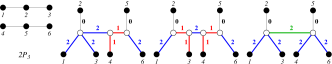
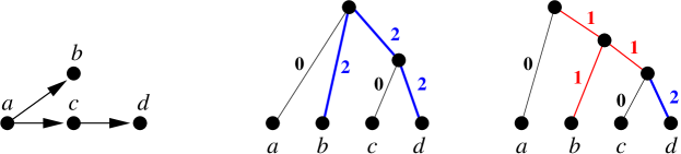
We note that connectedness of is necessary in Lemma 23 since for non-connected , the connected components can be “glued together” with arbitrarily complex trees as long as the distances between the attachment points is at least . In such examples it can be possible to contract edges without changing the explained graph. There are, for example at least three topologically different canonical trees that explain , see Fig. 8.
Lemma 24.
Let be a canonical tree explaining a connected graph and let be an interior vertex in . Then all edges incident to are 1-edges or has at least one adjacent leaf with .
Proof.
Suppose has no incident leaf. Since is connected, for every edge there is another edge such that . For this pair of edges we have because no interior edges is -labeled. Thus for all incident with . On the other hand, if has a neighbor with , then connectedness of implies that there is another neighbor of with . Hence, unless has only -neighbors, then there must be a least one incident -edge, which by assumption must be a leaf. ∎
We remark, finally, that a tree with minimal number of vertices (or edges) that explains a graph with respect to the exactly--relation is necessarily canonical. Otherwise, the contraction of an edge would make it possible to decrease of both the number of edges and vertices.
4 Oriented Exactly-2-Relation
Generalizing the construction of the oriented exactly-1-relation in [15], we consider here an oriented version of the exactly--relation. In constrast to the previous sections, we consider here rooted trees with leaf set . For two leaves and there is a unique least common ancestor, denoted by , defined as the vertex most distant from the root of that is common to the paths connecting with and with , respectively.
Definition 25.
Let be a rooted tree with leaf set and
edge-labeling function .
For we consider the directed exactly--relation
defined by if
and
holds for the the
(unique) paths from to and
from to , respectively.
The rooted tree explains a the
directed graph (with respect to the
directed exactly--relation) if if and only if
.
By construction is an oriented graph, i.e., at most one of and can be an edge. As in the unrooted case, we say that a rooted tree is canonical if it is a rooted phylogenetic tree and does not have an inner 0-edge. In the following we will consider the case that is discrete. As in the undirected case, we shall relax this requirement in the end.
As in [15], our strategy is to exploit the close relationships between the oriented and the undirected case. Therefore, we first derive some technical results regarding common properties of the oriented relation and its undirected relative .
Note that the underlying tree of a rooted canonical tree is not necessarily an unrooted canonical tree. By contracting all the interior 0-edges and degree 2 vertices, we get a unique unrooted canonical tree corresponds to . Conversely, for any unrooted canonical tree with , we can create a set of corresponding rooted least resolved trees as follows: (i) each interior vertex of may serve as a root; (ii) each leaf attached by a 0-edge may serve as a root; and (iii) every 2-edge can be subdivided by inserting a the root as a new vertex such that each of the two resulting edges is labeled 1. The construction is detailed in Algorithm 3. An example is given in Figure 9. The following lemma formalizes this one-to-one correspondence between unrooted canonical trees and its corresponding sets of rooted canonical tree.
Lemma 26.
Every rooted canonical tree can be constructed from its underlying unrooted canonical tree by Algorithm 3.
Proof.
By construction, the set of canonical rooted trees corresponding to unrooted canonical tree is well defined, i.e., the correspondence is a mapping.
Suppose there are two distinct unrooted canonical trees and such that both their correspondings sets of rooted trees contains . By construction, it has a underlying tree from which a unique canonical tree is obtained by contracting 0-edges and degree 2 vertices. Thus , a contradiction. Hence the mapping is injective.
The mapping is also surjective, since each rooted canonical tree can be constructed from its corresponding unrooted canonical tree. ∎
Lemma 27.
Suppose the unrooted canonical tree explains with respect to . Let be a digraph explained w.r.t. by a rooted tree corresponding to . Then the underlying graph of is a spanning subgraph of .
Proof.
By construction, and has the same leaf set, and hence .
Any arc in is an edge in the underlying graph of because that fact that explains implies and . Considering the underlying unrooted graph , we have . Since explains , and by construction displays , we conclude that also explains . Hence . ∎
Definition 28.
Suppose there a tree with discrete that explains w.r.t. , then every subgraph of is allowed for . Analogously, if there is a rooted tree with discrete that explains w.r.t. , we say that every subgraph of is allowed for .
In more detail a graph is allowed for if there exists such that for any , we have . If is not allowed for , we say that is it is forbidden (as a subgraph) for . Analogous, a graph is allowed for in the rooted case, if there exists such that for any , we have and . If is not allowed as a subgraph in , we that say is forbidden (as a subgraph) for in .
Lemma 29.
If is forbidden for , then any orientation of is forbidden in . If is allowed as a subgraph for with rooted tree , then its underlying graph is allowed for as a subgraph with the corresponding underlying tree .
Proof.
Suppose, for contradictions, that is forbidden for but the orientation of is allowed for . Then there exists a rooted tree such that for any arc in , we have and where . Consider the unrooted tree of . Since if and only if or is an arc in , then for any , and where . By definition, is allowed for , i.e., we arrive at a contradiction. The second statement is a simple consequence of the first one. ∎
The technical results obtained so far will allow us to infer properties of the oriented graph and their explaining trees from their underlying undirected graphs and unrooted trees . In the following we will focus on graphs that can be explained w.r.t. by a rooted tree with discrete .
Lemma 30.
Oriented cycles are forbidden as a subgraph for .
Proof.
Suppose is allowed. Then, by definition, there exists an orientation graph with vertex set such that is a subgraph of and a rooted tree that explains . W.l.o.g., we assume is a rooted canonical tree.
Consider the underlying unrooted canonical tree of , we claim that must be . Suppose that explains graph . By Lemma 27 since the underlying graph of is a subgraph of which has the same vertex set with , and contains a Hamiltonian cycle, thus also contains a Hamiltonian cycle, by Lemma 18 is a complete graph . And by Lemma 14 the displays .
Then we consider all the possibility to construct the set of rooted canonical trees corresponding to , and consider the oriented graph it explains. By Algorithm 3 we can place the root either on the center vertex, which will explain an empty graph, or place it on one of the leaves, which will explains oriented star on vertices point to the leaves. In either case there is no cycles. By Lemma 26 we know we have constructed all rooted canonical trees and thus all oriented graphs they explain. Thus oriented cycles are forbidden as a subgraph for . ∎
Lemma 31.
2-star oriented to center, , is forbidden as an induced subgraph for .
Proof.
Explicit construction shows that we obtain for each of the three triples , , and . This contradicts the assumption that is discrete. ∎
Lemma 32.
Every graph that can be explained by an edge-labeled tree w.r.t. is an oriented forest with the property that all its component trees have a unique source vertex from which all arcs are directed away.
Proof.
Let be a graph that can be explained w.r.t. . Since all cycles are forbidden induced subgraphs, is a forest. Furthermore, there is only a single source vertex in each connected component. Otherwise, if both and were sources within the same component tree, then the unique path from to would necessarily contain an induced subgraph of the form , which is forbidden. ∎
A canonical tree with discrete that explains a connected oriented graph w.r.t. has a leaf that is attached to the root by 0-edge.
Theorem 33.
is explained w.r.t. by a rooted tree with discrete if and only if is an oriented forest that does not contain the 2-star oriented to center, , as an induced subgraph.
Proof.
To show the “only if” part, suppose can be explained. Then is oriented and by Lemma 30 it is an orientation tree, and by Lemma 31 we know that 2-star oriented to center is forbidden. For the “if” part we use the construction employed in [15] for (with 2-edges taking the place of 1-edges): To each inner vertex of a new vertex which represent in tree is attached with a 0-edge, while the inner edges of the tree have label . The Theorem now follows directly from Lemma 4. ∎
We can relax the condition that has discrete . To this end, we extend the false twin relation to digraphs by setting iff and have the same in- and out-neighbors. The quotient graph is known as the point-determining graph of .
Corollary 34.
An oriented graph is explained w.r.t. if and only if is an oriented forest whose point-determining graph does not contain as an induced subgraph.
Proof.
It suffices to note that -equivalent vertices are in the same -class and that there is a least resolved tree in which all members of a -class are siblings. ∎
We note, finally, that the rooted trees with discrete that explain w.r.t. are not unique, as exemplified in Figure 10.
5 Concluding Remarks
The main result of this contribution is the characteriztion of the exactly--relations, i.e. the graphs . They form a proper superset of the the exact-2-leaf power graphs, which comprise only the disjoint unions of cliques. Section 2 suggests, however, that at least some of the structure and techniques carry over to general values of . Several related problems are worth considering as well: in particular, and are of interest as models for coarse grained models of evolutionary distances.
The oriented version of the exactly--relation somewhat surprisingly, is much more closely related to the oriented exactly--relation of [15] that to the undirected exactly--relation. There is an alternative natural definition for a directed exactly--relation that omit the condition that . Clearly, the resulting digraph are not oriented, i.e., they may contain double edged. We suspect that their structure is more closely related to the Fitch graph (directed at-least--relation) recently studied in [17].
Regarding the analysis of rare-event data in phylogenetics the characterization of the exactly--relation naturally leads to the edge modification problem for block graphs and graphs whose R-thin quotient is a block graph, respectively. Although these problems do not seem to have been studied so far (see e.g. [37, Tab.1] and [38]). Since exactly-2-relation graphs are hereditary by Lemma 3, we suspect that edge modification problem for the exactly-2-relation graphs can be handled in manner similar to closely related edge modification problem for chordal graphs [37, 38] or cluster editing [39].
Acknowledgments
The authors gratefully acknowledge stimulating discussions with Marc Hellmuth, Manuela Geiß, and Maribel Hernández-Rosales on related classes of graphs derived from labeled trees.
References
- [1] C. Semple, M. Steel, Phylogenetics, Oxford University Press, Oxford UK, 2003.
- [2] A. W. M. Dress, K. T. Huber, J. Koolen, V. Moulton, A. Spillner, Basic Phylogenetic Combinatorics, Cambridge University Press, Cambridge UK, 2012.
- [3] P. E. Kearney, J. I. Munro, D. Phillips, Efficient generation of uniform samples from phylogenetic trees, in: Algorithms in Bioinformatics (WABI 2003 Budapest), Vol. 2812 of Lect. Notes Comp. Sci., Springer, Berlin, 2003, pp. 177–189. doi:10.1007/978-3-540-39763-2\_14.
- [4] M. N. Yanhaona, K. S. M. T. Hossain, M. S. Rahman, Pairwise compatibility graphs, J. Appl. Math. Comput. 30 (2009) 479–503. doi:10.1007/s12190-008-0204-7.
- [5] T. Calamoneri, B. Sinaimeri, Pairwise compatibility graphs: A survey, SIAM Review 58 (2016) 445–460. doi:10.1137/140978053.
- [6] M. I. Hossain, S. A. Salma, M. S. Rahman, D. Mondal, A necessary condition and a sufficient condition for pairwise compatibility graphs, J. Graph Algorithms Appl. 21 (2017) 341–352. doi:10.1007/978-3-319-30139-6\_9.
- [7] P. Baiocchi, T. Calamoneri, A. Monti, R. Petreschi, Graphs that are not pairwise compatible: A new proof technique, in: C. Iliopoulos, H. W. Leong, W.-K. Sung (Eds.), Combinatorial Algorithms, 29th IWOCA, Vol. 10979 of Lecture Notes Comp. Sci., Springer, Berlin, Heidelberg, 2018, pp. 39–51. doi:10.1007/978-3-319-94667-2\_4.
- [8] P. Baiocchi, T. Calamoneri, A. Monti, R. Petreschi, Some classes of graphs that are not PCGs, Theor. Comp. Sci. 791 (2019) 62–75. doi:10.1016/j.tcs.2019.05.017.
- [9] S. Ahmed, M. S. Rahman, Multi-interval pairwise compatibility graphs, in: T. V. Gopal, G. Jäger, S. Steila (Eds.), Theory and Applications of Models of Computation (14’th TAMC 2017), Vol. 10185 of Lect. Notes Comp. Sci., Springer, Heidelberg, 2017, pp. 71–84. doi:10.1007/978-3-319-55911-7\_6.
- [10] A. Brandstädt, V. B. Lea, D. Rautenbach, Exact leaf powers, Theor. Comp. Sci. 411 (2010) 2968–2977. doi:10.1016/j.tcs.2010.04.027.
- [11] A. Rokas, P. W. Holland, Rare genomic changes as a tool for phylogenetics, Trends Ecol Evol 15 (2000) 454–459. doi:10.1016/S0169-5347(00)01967-4.
- [12] J. E. Tarver, E. A. Sperling, A. Nailor, A. M. Heimberg, J. M. Robinson, B. L. King, D. Pisani, P. C. J. Donoghue, K. J. Peterson, miRNAs: Small genes with big potential in metazoan phylogenetics, Mol. Biol. Evol. 30 (2013) 2369–2382. doi:10.1093/molbev/mst133.
- [13] H. Luo, W. Arndt, Y. Zhang, G. Shi, M. A. Alekseyev, J. Tang, A. L. Hughes, R. Friedman, Phylogenetic analysis of genome rearrangements among five mammalian orders, Mol Phylogenet Evol. 65 (2012) 871–882. doi:10.1016/j.ympev.2012.08.008.
- [14] J. W. Waegele, T. W. Bartholomaeus (Eds.), Deep Metazoan Phylogeny: The Backbone of the Tree of Life—New Insights from Analyses of Molecules, Morphology, and Theory of Data Analysis, De Gruyter, 2014.
- [15] M. Hellmuth, M. Hernandez-Rosales, Y. Long, P. F. Stadler, Inferring phylogenetic trees from the knowledge of rare evolutionary events, J. Math. Biol. 76 (2017) 1623–1653. doi:10.1007/s00285-017-1194-6.
- [16] M. Hellmuth, Y. Long, M. Geiß, P. F. Stadler, A short note on undirected Fitch graphs, Art Discrete Appl. Math. (ADAM) 1 (2018) P1.08. doi:10.26493/2590-9770.1245.98c.
- [17] M. Geiß, J. Anders, P. F. Stadler, N. Wieseke, M. Hellmuth, Reconstructing gene trees from Fitch’s xenology relation, J. Math. Biol. 77 (2017) 1459–1491. doi:10.1007/s00285-018-1260-8.
- [18] C. Crespelle, C. Paul, Fully dynamic recognition algorithm and certificate for directed cographs, Discr. Appl. Math. 154 (2006) 1722–1741. doi:10.1016/j.dam.2006.03.005.
- [19] K. Chaudhuri, K. Chen, R. Mihaescu, S. Rao, On the tandem duplication-random loss model of genome rearrangement, in: Proc. 17th Ann. ACM-SIAM Symp. Discrete Algorithm (SODA ’06), Soc. Industrial Appl. Math., Philadelphia, 2006, pp. 564–570. doi:10.5555/1109557.1109619.
- [20] M. Hellmuth, M. Hernandez-Rosales, K. T. Huber, V. Moulton, P. F. Stadler, N. Wieseke, Orthology relations, symbolic ultrametrics, and cographs, J. Math. Biol. 66 (2013) 399–420. doi:10.1007/s00285-012-0525-x.
- [21] N. Nishimura, P. Ragde, D. M. Thilikos, On graph powers for leaf-labeled trees, J. Algorithms 42 (2002) 69–108. doi:10.1006/jagm.2001.1195.
- [22] T. Calamoneri, E. Montefusco, R. Petreschi, B. Sinaimeria, Exploring pairwise compatibility graphs, Theor. Comp. Sci. 468 (2013) 23–36. doi:10.1016/j.tcs.2012.11.015.
- [23] P. Buneman, The recovery of trees from measures of dissimilarity, in: F. R. Hodson, D. G. Kendall, P. Tautu (Eds.), Mathematics in the Archaeological and Historical Sciences, Edinburgh University Press, Edinburgh, 1971, pp. 387–385.
- [24] J. M. S. Simões-Pereira, A note on the tree realizability of a distance matrix, J. Combin. Theory 6 (1969) 303–310. doi:10.1016/S0021-9800(69)80092-X.
- [25] H.-J. Bandelt, H. M. Mulder, Distance-hereditary graphs, J. Comb. Th., Ser. B 41 (1986) 182–208. doi:10.1016/0095-8956(86)90043-2.
- [26] R. Hammack, W. Imrich, S. Klavžar, Handbook of Product graphs, 2nd Edition, CRC Press, Boca Raton, 2011.
- [27] R. McKenzie, Cardinal multiplication of structures with a reflexive relation, Fund. Math. 70 (1971) 59–101. doi:10.4064/fm-70-1-59-101.
- [28] D. P. Sumner, Point determination in graphs, Discrete Math. 5 (1973) 179–187. doi:10.1016/0012-365X(73)90109-X.
- [29] J. J. Bull, C. M. Pease, Combinatorics and variety of mating-type systems, Evolution 43 (1989) 667–671. doi:10.1111/j.1558-5646.1989.tb04263.x.
- [30] G. Kilibarda, Enumeration of unlabelled mating graphs, Graphs Combinatorics 23 (2007) 183–199. doi:10.1007/s00373-007-0692-5.
- [31] I. Gessel, J. Li, Enumeration of point-determining graphs, J. Comb. Th., Ser. A 118 (2011) 591–612. doi:10.1016/j.jcta.2010.03.009.
- [32] W. Imrich, Factoring cardinal product graphs in polynomial time, Discrete Math. 192 (1998) 119–144. doi:10.1016/S0012-365X(98)00069-7.
- [33] A. Brandstädt, C. Hundt, Ptolemaic graphs and interval graphs are leaf powers, in: E. S. Laber, C. F. Bornstein, L. T. Nogueira, F. L. (Eds.), LATIN 2008, Vol. 4957 of Lect. Notes Comp. Sci., Springer, Berlin, 2008, pp. 479–491. doi:10.1007/978-3-540-78773-0\_42.
- [34] T. Calamoneri, A. Frangioni, B. Sinaimeri, Pairwise compatibility graphs of caterpillars, Computer J. 57 (2014) 1616–1623. doi:10.1093/comjnl/bxt068.
- [35] S. A. Salma, M. S. Rahman, M. I. Hossain, Triangle-free outerplanar 3-graphs are pairwise compatibility graphs, J. Graph Alg. Appl. 17 (2013) 81–102. doi:10.7155/jgaa.00286.
- [36] F. Harary, A characterization of block-graphs, Canadian Math. Bull. 6 (1963) 1–6. doi:10.4153/CMB-1963-001-x.
- [37] P. Burzyn, F. Bonomo, G. Durán, NP-completeness results for edge modification problems, Discr. Appl. Math. 154 (2006) 1824–1844. doi:10.1016/j.dam.2006.03.031.
- [38] R. Sritharan, Graph modification problem for some classes of graphs, J. Discr. Algorithms 38-41 (2016) 32–37. doi:10.1016/j.jda.2016.06.003.
- [39] R. Shamir, R. Sharan, D. Thur, Cluster graph modification problems, Discr. Appl. Math. 144 (2004) 173–182. doi:10.1016/j.dam.2004.01.007.