This paper was converted on www.awesomepapers.org from LaTeX by an anonymous user.
Want to know more? Visit the Converter page.

Exact distributed quantum algorithm for generalized Simon’s problem

Hao Li, Daowen Qiu $†$ issqdw@mail.sysu.edu.cn (D.W. Qiu, Corresponding author’s address) Institute of Quantum Computing and Computer Theory, School of Computer Science and Engineering, Sun Yat-sen University, Guangzhou 510006, China;
The Guangdong Key Laboratory of Information Security Technology, Sun Yat-sen University, 510006, China;
QUDOOR Technologies Inc., Zhuhai, China
   Le Luo School of Physics and Astronomy, Sun Yat-sen University, 519082 Zhuhai, China;
QUDOOR Technologies Inc., Zhuhai, China
   Paulo Mateus Instituto de Telecomunicações, Departamento de Matemática, Instituto Superior Técnico, Av. Rovisco Pais 1049-001 Lisbon, Portugal
(August 27, 2025)
Abstract

Simon’s problem is one of the most important problems demonstrating the power of quantum algorithms, as it greatly inspired the proposal of Shor’s algorithm. The generalized Simon’s problem is a natural extension of Simon’s problem, and also a special hidden subgroup problem: Given a function f:{0,1}n{0,1}mf:{\{0,1\}}^{n}\to{\{0,1\}}^{m}, with the property that for any x,y{0,1}nx,y\in{\{0,1\}}^{n}, there is some unknown hidden subgroup S2nS\leq\mathbb{Z}_{2}^{n} such that f(x)=f(y)f(x)=f(y) iff xySx\oplus y\in S, where |S|=2k|S|=2^{k} for some 0kn0\leq k\leq n (mnk)(m\geq n-k). The goal of generalized Simon’s problem is to find the hidden subgroup SS. In this paper, we present two key contributions. Firstly, we characterize the structure of the generalized Simon’s problem in distributed scenario and introduce a corresponding distributed quantum algorithm. Secondly, we refine the algorithm to ensure exactness due to the application of quantum amplitude amplification technique. Our algorithm offers exponential acceleration compared to the distributed classical algorithm. When contrasted with the centralized quantum algorithm for the generalized Simon’s problem, our algorithm’s oracle requires fewer qubits, thus making it easier to be physically implemented. Particularly, the exact distributed quantum algorithm we develop for the generalized Simon’s problem outperforms the best previously proposed distributed quantum algorithm for Simon’s problem in terms of generalizability and exactness.

pacs:
Valid PACS appear here
preprint: APS/123-QED

I INTRODUCTION

Quantum computing nielsen_quantum_2010 has been proved to have great potential in factorizing large numbers shor_polynomial-time_1997 , searching unordered database grover_fast_1996 and solving linear systems of equations HHL_2009 . However, large-scale universal quantum computers have not yet been realized due to the limitations of current physical devices. At present, quantum technology has been entered to the Noisy Intermediate-Scale Quantum (NISQ) era preskill_quantum_2018 , which makes it possible to implement quantum algorithms on middle-scale circuits.

Distributed quantum computing is a novel computing architecture, which combines quantum computing with distributed computing goos_distributed_2003 ; beals_efficient_2013 ; Qiu2017DQC ; caleffi_quantum_2018 ; avron_quantum_2021 ; Qiu22 ; Tan2022DQCSimon ; Xiao2023DQAShor ; Hao2023DDJ ; Xiao2023DQAkShor . In distributed quantum computing architecture, multiple quantum computing nodes communicate with each other and cooperate to complete computing tasks. Compared with centralized quantum computing, the size and depth of circuit can be reduced by using distributed quantum computing, which is beneficial to improve the performance of circuit against noise.

Simon’s problem is one of the most important problems in quantum computing simon_power_1997 . For solving Simon’s problem, quantum algorithms have the advantage of exponential acceleration over classical algorithms cai_optimal_2018 . Remarkably, Simon’s algorithm greatly inspired the proposal of Shor’s algorithm shor_polynomial-time_1997 . Furthermore, the generalized Simon’s problem is a natural extension of Simon’s problem, and an instance of the hidden subgroup problem nielsen_quantum_2010 ; kaye_introduction_2007 .

Tan, Xiao, and Qiu et al. Tan2022DQCSimon proposed a distributed quantum algorithm for Simon’s problem, but they left it open as to whether an exact distributed version exists. In the centralized case, Cai and Qiu cai_optimal_2018 utilized quantum amplitude amplification to address the issue of exactness for Simon’s problem. Their approach has served as inspiration for our work. In this paper, we contribute in two new ways. Firstly, we characterize the structure of the generalized Simon’s problem in distributed scenario and leverage this understanding to design a corresponding distributed quantum algorithm. Secondly, we incorporate quantum amplitude amplification BHMT02 to ensure the algorithm’s exactness.

The remainder of this paper is organized as follows. In Sec. II, we present some notations related to group theory, and recall the generalized Simon’s problem. In Sec. III, we characterize the structure of the generalized Simon’s problem in distributed scenario. Then, in Sec. IV we describe a distributed quantum algorithm for the generalized Simon’s problem and give the corresponding analytical procedure. Furthermore, in Sec. V we introduce quantum amplitude amplification technique, and with this technique, we in Sec. VI design an exact distributed quantum algorithm for the generalized Simon’s problem and prove its correctness. In addition, in Sec. VII, we compare our algorithm with other algorithms. Finally, we conclude with a summary in Sec. VIII.

II PRELIMINARIES

In this section, we present some notations related to group theory, and recall the generalized Simon’s problem.

II.1 Notations

It is known that the generalized Simon’s problem is an instance of the hidden subgroup problem. Below, we present some of the notations related to group theory.

For x,y2nx,y\in\mathbb{Z}_{2}^{n} with x=(x1,,xn)x=(x_{1},\ldots,x_{n}) and y=(y1,,yn)y=(y_{1},\ldots,y_{n}), we define

x+y((x1+y1)mod2,,(xn+yn)mod2).\displaystyle x+y\coloneqq((x_{1}+y_{1})\bmod 2,\ldots,(x_{n}+y_{n})\bmod 2). (1)
xy(x1y1++xnyn)mod2.\displaystyle x\cdot y\coloneqq(x_{1}\cdot y_{1}+\cdots+x_{n}\cdot y_{n})\bmod 2. (2)

For any subset X2nX\subseteq\mathbb{Z}_{2}^{n}, X\langle X\rangle denotes the subgroup generated by XX, i.e.,

X{i=1kαixi|xiX,αi{0,1}}.\langle X\rangle\coloneqq\left\{\sum_{i=1}^{k}\alpha_{i}x_{i}|x_{i}\in X,\alpha_{i}\in\{0,1\}\right\}. (3)

The set XX is linearly independent if XY\langle X\rangle\neq\langle Y\rangle for any proper subset YY of XX. Notice that the cardinality |X||\langle X\rangle| is 2|X|2^{|X|} if XX is linearly independent.

Let GG denote the group ({0,1},)(\{0,1\},\oplus), the basis of GG is a maximal linearly independent subset of GG. The cardinality of the basis of GG is called its rankrank, denoted by rank(G)rank(G). If HH is a subgroup of GG, then we denote HGH\leq G. For HGH\leq G, let

H{gG|gh=0,hH}.H^{\perp}\coloneqq\{g\in G|g\cdot h=0,\forall h\in H\}. (4)

Notice that (H)=H(H^{\perp})^{\perp}=H and |H|=2n|H||\langle H\rangle^{\perp}|=2^{n-|H|} if HH is linearly independent.

II.2 The generalized Simon’s problem

The generalized Simon’s problem is a special kind of the hidden subgroup problem kaye_introduction_2007 , which can be described as follows. Consider a function f:{0,1}n{0,1}mf:\{0,1\}^{n}\rightarrow\{0,1\}^{m}, where we promise that for any x,y{0,1}nx,y\in{\{0,1\}}^{n}, there is a hidden subgroup S2nS\leq\mathbb{Z}_{2}^{n}, such that f(x)=f(y)f(x)=f(y) if and only if xySx\oplus y\in S, where |S|=2k|S|=2^{k} for some 0kn0\leq k\leq n (mnk)(m\geq n-k). For the specific case where k=1k=1, the generalized Simon’s problem precisely aligns with Simon’s problem.

Denote the basis of SS as {si|si{0,1}n,1ik}\{s_{i}|s_{i}\in\{0,1\}^{n},1\leq i\leq k\}, then we have

S={i=1kαisi|si{0,1}n,αi{0,1}}.S=\left\{\sum_{i=1}^{k}\alpha_{i}s_{i}\Bigg{|}s_{i}\in\{0,1\}^{n},\alpha_{i}\in\{0,1\}\right\}. (5)

Suppose we have an oracle that can query the value of function ff. For any x{0,1}nx\in\{0,1\}^{n} and any b{0,1}mb\in\{0,1\}^{m}, if we input |x|b|x\rangle|b\rangle into the oracle, then |x|bf(x)|x\rangle|b\oplus f(x)\rangle is obtained.The goal of the generalized Simon’s problem is to find the hidden subgroup SS by performing the minimum number of queries to function ff.

The quantum query complexity of the generalized Simon’s problem is Θ(nk)\Theta(n-k). The lower bound on the classical (deterministic or randomized) query complexity of the generalized Simon’s problem is Ω(max{k,2nk})\Omega\left(\max\left\{k,\sqrt{2^{n-k}}\right\}\right), and its upper bound on the classical query complexity is O(max{k,k2nk})O\left(\max\left\{k,\sqrt{k\cdot 2^{n-k}}\right\}\right) WuGSP ; KunGSP .

III the generalized Simon’s problem in the distributed scenario

In the following, we describe the generalized Simon’s problem in distributed scenario and characterize its structure.

The function ff corresponding to the generalized Simon’s problem is divided into 2t2^{t} subfunctions fw:{0,1}nt{0,1}mf_{w}:\{0,1\}^{n-t}\rightarrow\{0,1\}^{m} as follows. Let

fw(u)=f(uw),f_{w}(u)=f(uw), (6)

where u{0,1}ntu\in\{0,1\}^{n-t}, w{0,1}tw\in\{0,1\}^{t}.

Suppose there are 2t2^{t} people, each of whom has an oracle OfwO_{f_{w}} that can query all fw(u)=f(uw)f_{w}(u)=f(uw) for any u{0,1}ntu\in\{0,1\}^{n-t}, w{0,1}tw\in\{0,1\}^{t}, where OfwO_{f_{w}} are defined as

Ofw|u|b=|u|bfw(u),O_{f_{w}}\ket{u}\ket{b}=\ket{u}\ket{b\oplus f_{w}(u)}, (7)

where u{0,1}ntu\in\{0,1\}^{n-t}, w{0,1}tw\in\{0,1\}^{t} and b{0,1}mb\in\{0,1\}^{m}.

Each person can access 2nt2^{n-t} values of ff. They need to find the hidden subgroup SS by querying their own oracle and communicating with each other as few times as possible.

Below, we further introduce some notations related to the function ff corresponding to the generalized Simon’s problem. We anticipate that the reader is already familiar with the concept of multisets.

Definition 1.

For any u{0,1}ntu\in\{0,1\}^{n-t}, let G(u)G(u) denote the multiset {fw(u)|w{0,1}t}\{f_{w}(u)|w\in\{0,1\}^{t}\}.

Definition 2.

For any u{0,1}ntu\in\{0,1\}^{n-t}, let N(u,z)={w{0,1}t|zG(u),fw(u)=z}N(u,z)=\{w\in\{0,1\}^{t}|z\in G(u),f_{w}(u)=z\}.

Definition 3.

For any u{0,1}ntu\in\{0,1\}^{n-t}, let S(u)S(u) represent a string of length 2tm2^{t}m by concatenating all strings fw(u)f_{w}(u) (w{0,1}t)(w\in\{0,1\}^{t}) according to lexicographical order, that is,

S(u)=fw0(u)fw1(u)fw2t1(u),\displaystyle S(u)=f_{w_{0}}(u)f_{w_{1}}(u)\cdots f_{w_{2^{t}-1}}(u), (8)

where fw0(u)fw1(u)fw2t1(u){0,1}mf_{w_{0}}(u)\leq f_{w_{1}}(u)\leq\ldots\leq f_{w_{2^{t}-1}}(u)\in\{0,1\}^{m}, with wi{0,1}tw_{i}\in\{0,1\}^{t} (0i2t1)(0\leq i\leq 2^{t}-1), where wiwjw_{i}\neq w_{j} for any iji\neq j and \leq denotes the lexicographical order.

Let SS be the hidden subgroup to be found, and denote the basis of SS as {silsir|si=silsir,si{0,1}n,sil{0,1}nt,sir{0,1}t,1ik}\{s_{il}s_{ir}|s_{i}=s_{il}s_{ir},s_{i}\in\{0,1\}^{n},s_{il}\in\{0,1\}^{n-t},s_{ir}\in\{0,1\}^{t},1\leq i\leq k\}.

Let

Sl={i=1kαisil|sil{0,1}nt,αi{0,1}},S_{l}=\left\{\sum_{i=1}^{k}\alpha_{i}s_{il}\Bigg{|}s_{il}\in\{0,1\}^{n-t},\alpha_{i}\in\{0,1\}\right\}, (9)

then Sl2ntS_{l}\leq\mathbb{Z}_{2}^{n-t}.

Denote kl=rank(Sl)k_{l}=rank(S_{l}), 0klmin(k,nt)0\leq k_{l}\leq\min(k,n-t), and the basis of SlS_{l} as {ei|ei{0,1}nt,1ikl}\left\{e_{i}|e_{i}\in\{0,1\}^{n-t},1\leq i\leq k_{l}\right\}.

Let

Sr={i=1kαisir|sir{0,1}t,αi{0,1}},S_{r}=\left\{\sum_{i=1}^{k}\alpha_{i}s_{ir}\Bigg{|}s_{ir}\in\{0,1\}^{t},\alpha_{i}\in\{0,1\}\right\}, (10)

then Sr2tS_{r}\leq\mathbb{Z}_{2}^{t}.

The following theorem concerning S(u)S(u) is useful and important.

Theorem 1.

Suppose function f:{0,1}n{0,1}mf:\{0,1\}^{n}\rightarrow\{0,1\}^{m}, satisfies that there is a subgroup S2nS\leq\mathbb{Z}_{2}^{n} such that f(x)=f(y)f(x)=f(y) if and only if xySx\oplus y\in S. Then u,v{0,1}nt,S(u)=S(v)\forall u,v\in\{0,1\}^{n-t},S(u)=S(v) if and only if uvSlu\oplus v\in S_{l}.

Proof.

Based on the properties of multiset, u,v{0,1}nt,S(u)=S(v)\forall u,v\in\{0,1\}^{n-t},S(u)=S(v) if and only if G(u)=G(v)G(u)=G(v). So our goal is to prove u,v{0,1}nt,G(u)=G(v)\forall u,v\in\{0,1\}^{n-t},G(u)=G(v) if and only if uvSlu\oplus v\in S_{l}.

(1) \Longleftarrow. First, we prove if uvSlu\oplus v\in S_{l}, then G(u)G(v)G(u)\subseteq G(v). We have zG(u),wN(u,z)\forall z\in G(u),\exists w\in N(u,z) such that z=f(uw)z=f(uw). According to the definition of the generalized Simon’s problem, sS\forall s\in S, f(uws)=f(uw)=zf(uw\oplus s)=f(uw)=z. In addition, we have sS\forall s\in S, slSl\exists s_{l}\in S_{l}, srSrs_{r}\in S_{r} such that s=slsrs=s_{l}s_{r}.

Thus, we have sS\forall s\in S, z=f(uws)=f((usl)(wsr))z=f(uw\oplus s)=f((u\oplus s_{l})(w\oplus s_{r})). By the definition of group SS and SlS_{l}, we have slSl\forall s_{l}\in S_{l} and slsrSs_{l}s_{r}\in S, z=f((usl)(wsr))z=f((u\oplus s_{l})(w\oplus s_{r})). Since uvSlu\oplus v\in S_{l}, there slSl\exists s_{l}\in S_{l} such that usl=vu\oplus s_{l}=v. Hence, we have z=f(v(wsr))G(v)z=f(v(w\oplus s_{r}))\in G(v). Therefore, G(u)G(v)G(u)\subseteq G(v) and |N(u,z)||N(v,z)||N(u,z)|\leq|N(v,z)|. Similarly, we can prove that G(v)G(u)G(v)\subseteq G(u) and |N(v,z)||N(u,z)||N(v,z)|\leq|N(u,z)|. As a result, we have G(u)=G(v)G(u)=G(v).

(2) \Longrightarrow. Since G(u)=G(v)G(u)=G(v), we have zG(u),zG(v)\forall z\in G(u),z\in G(v). Then we have w,w{0,1}t\exists w,w^{\prime}\in\{0,1\}^{t} such that z=f(uw)z=f(uw) and z=f(vw)z=f(vw^{\prime}). So we have f(uw)=f(vw)f(uw)=f(vw^{\prime}). According to the definition of the generalized Simon’s problem, we have uwvw=(uv)(ww)Suw\oplus vw^{\prime}=(u\oplus v)(w\oplus w^{\prime})\in S. Further, by the definition of group SS and SlS_{l}, we have uvSlu\oplus v\in S_{l}. ∎

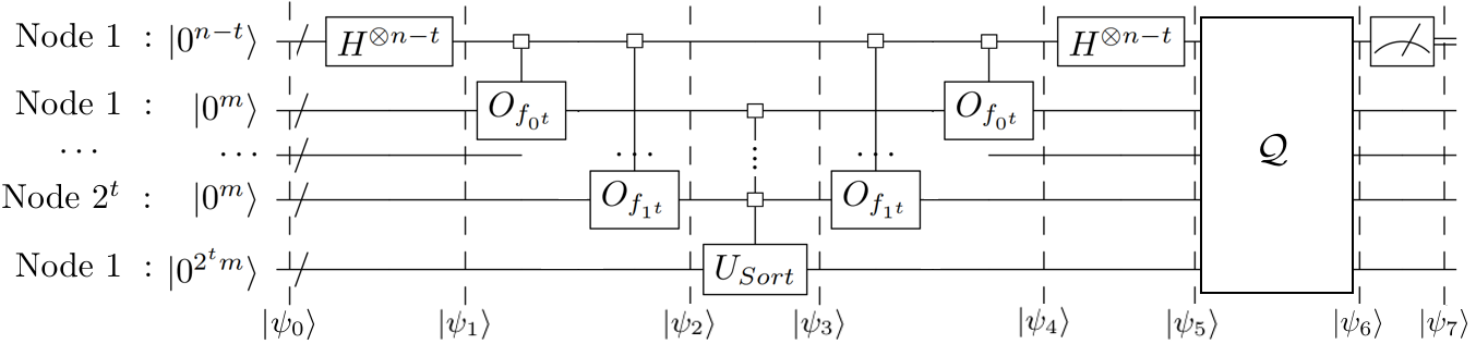
IV Distributed quantum algorithm for the generalized Simon’s problem

In the following, we begin with giving related notation, function and operators that are used in distributed quantum algorithm for the generalized Simon’s problem, i.e., Algorithm 1.

Let [N][N] represent the set of integers {0,1,,2t1}\{0,1,\cdots,2^{t}-1\}, and let BI:{0,1}t[N]{\rm BI}:\{0,1\}^{t}\rightarrow[N] be the function to convert a binary string of tt bits to an equal decimal integer.

The query operators OfwO^{\prime}_{f_{w}} in Algorithm 1 are defined as

Ofw|u|b|c=|u|b|cfw(u),O^{\prime}_{f_{w}}\ket{u}\ket{b}\ket{c}=\ket{u}\ket{b}\ket{c\oplus f_{w}(u)}, (11)

where u{0,1}ntu\in\{0,1\}^{n-t}, w{0,1}tw\in\{0,1\}^{t}, b{0,1}BI(w)b\in\{0,1\}^{{\rm BI}(w)} and c{0,1}mc\in\{0,1\}^{m}.

The operator USort:{0,1}2t+1m{0,1}2t+1mU_{Sort}:\{0,1\}^{2^{t+1}m}\rightarrow\{0,1\}^{2^{t+1}m} in Algorithm 1 is defined as

USort(w{0,1}t|fw(u))|b=(w{0,1}t|fw(u))|bS(u),\begin{split}&U_{Sort}\left(\bigotimes_{w\in\{0,1\}^{t}}\ket{f_{w}(u)}\right)|b\rangle\\ =&\left(\bigotimes_{w\in\{0,1\}^{t}}\ket{f_{w}(u)}\right)\Ket{b\oplus S(u)},\end{split} (12)

where w{0,1}t|fw(u)|f0t(u)|f0t11(u)|f1t(u)\bigotimes\limits_{w\in\{0,1\}^{t}}\ket{f_{w}(u)}\triangleq\ket{f_{0^{t}}(u)}\ket{f_{0^{t-1}1}(u)}\cdots\ket{f_{1^{t}}(u)} and b{0,1}2tmb\in\{0,1\}^{2^{t}m}.

Intuitively, the effect of USortU_{Sort} in Algorithm 1 is to sort the values in the 2t2^{t} control registers by lexicographical order and XOR to the target register.

In addition, for any operator AwA_{w} with w{0,1}tw\in\{0,1\}^{t}, we let w{0,1}tAwA1tA1t10A0t\prod_{w\in\{0,1\}^{t}}A_{w}\triangleq A_{1^{t}}A_{1^{t-1}0}\cdots A_{0^{t}}, w{0,1}tAwA0tA0t11\prod^{\prime}_{w\in\{0,1\}^{t}}A_{w}\triangleq A_{0^{t}}A_{0^{t-1}1} A1t\cdots A_{1^{t}}.

Algorithm 1 Distributed quantum algorithm for finding the elements in SlS_{l}^{\perp}
1:procedure DSL(integer nn, integer tt, integer mm, operator OfwO_{f_{w}})
2:  Y{0nt}Y\leftarrow\{0^{n-t}\};
3:  |ψ0=|0nt|02t+1m|\psi_{0}\rangle=\Ket{0^{n-t}}\Ket{0^{2^{t+1}m}};
4:  |ψ1=(HntI2t+1m)|ψ0|\psi_{1}\rangle=\left(H^{\otimes n-t}\otimes I^{\otimes 2^{t+1}m}\right)|\psi_{0}\rangle;
5:  |ψ2=w{0,1}t(OfwI2t+1mBI(w)mm)|ψ1\ket{\psi_{2}}=\prod_{w\in\{0,1\}^{t}}\left(O^{\prime}_{f_{w}}\otimes I^{\otimes 2^{t+1}m-{\rm BI}(w)\cdot m-m}\right)\ket{\psi_{1}};
6:  |ψ3=(IntUsort)|ψ2\ket{\psi_{3}}=\left(I^{\otimes{n-t}}\otimes U_{sort}\right)\ket{\psi_{2}};
7:  |ψ4=w{0,1}t(OfwI2t+1mBI(w)mm)|ψ3|\psi_{4}\rangle=\prod^{\prime}_{w\in\{0,1\}^{t}}\left(O^{\prime}_{f_{w}}\otimes I^{\otimes 2^{t+1}m-{\rm BI}(w)\cdot m-m}\right)\ket{\psi_{3}};
8:  |ψ5=(HntI2t+1m)|ψ4|\psi_{5}\rangle=\left(H^{\otimes n-t}\otimes I^{\otimes 2^{t+1}m}\right)|\psi_{4}\rangle;
9:  Measure the first register, and get an element zz;
10:  if zYz\notin\langle Y\rangle then
11:   YY{z}Y\leftarrow Y\cup\{z\}.
12:  end if
13:end procedure

In the following, we prove the correctness of Algorithm 1. The state after the third step of Algorithm 1 is

|ψ1=(HntI2t+1m)|ψ0=12ntu{0,1}nt|u|02t+1m.\begin{split}|\psi_{1}\rangle&=\left(H^{\otimes n-t}\otimes I^{\otimes 2^{t+1}m}\right)|\psi_{0}\rangle\\ &=\frac{1}{\sqrt{2^{n-t}}}\sum_{u\in\{0,1\}^{n-t}}|u\rangle\Ket{0^{2^{t+1}m}}.\end{split} (13)

Then Algorithm 1 queries each of the oracles to get the following state.

|ψ2=w{0,1}t(OfwI2t+1mBI(w)mm)|ψ1=12ntu{0,1}nt|u(w{0,1}t|fw(u))|02tm.\begin{split}\ket{\psi_{2}}=&\prod_{w\in\{0,1\}^{t}}\left(O^{\prime}_{f_{w}}\otimes I^{\otimes 2^{t+1}m-{\rm BI}(w)\cdot m-m}\right)\ket{\psi_{1}}\\ =&\frac{1}{\sqrt{2^{n-t}}}\sum_{u\in\{0,1\}^{n-t}}|u\rangle\left(\bigotimes_{w\in\{0,1\}^{t}}\ket{f_{w}(u)}\right)\Ket{0^{2^{t}m}}.\end{split} (14)

After sorting by using USortU_{Sort}, we have the following state.

|ψ3=(IntUsort)|ψ2=12ntu{0,1}nt|u(w{0,1}t|fw(u))|S(u).\begin{split}\ket{\psi_{3}}=&\left(I^{\otimes{n-t}}\otimes U_{sort}\right)\ket{\psi_{2}}\\ =&\frac{1}{\sqrt{2^{n-t}}}\sum_{u\in\{0,1\}^{n-t}}|u\rangle\left(\bigotimes_{w\in\{0,1\}^{t}}\ket{f_{w}(u)}\right)|S(u)\rangle.\end{split} (15)

After that, we query each oracle again and obtain the following state.

|ψ4=w{0,1}t(OfwI2t+1mBI(w)mm)|ψ3=12ntu{0,1}nt|u|02tm|S(u).\begin{split}|\psi_{4}\rangle=&\prod\nolimits_{w\in\{0,1\}^{t}}^{\prime}\left(O^{\prime}_{f_{w}}\otimes I^{\otimes 2^{t+1}m-{\rm BI}(w)\cdot m-m}\right)\ket{\psi_{3}}\\ =&\frac{1}{\sqrt{2^{n-t}}}\sum_{u\in\{0,1\}^{n-t}}|u\rangle\Ket{0^{2^{t}m}}|S(u)\rangle.\end{split} (16)

After using Hadamard transform on the first register, in the light of Theorem 1, we get the following state.

|ψ5=(HntI2t+1m)|ψ4=12ntu,z{0,1}nt(1)uz|z,02tm,S(u)=12nt|Sl|u,z{0,1}ntslSl(1)(usl)z|z,02tm,S(usl)=12nt+klu,z{0,1}ntslSl(1)uz(1)slz|z,02tm,S(u)=12nt+klu,z{0,1}nt(slSl(1)slz)(1)uz|z,02tm,S(u).\begin{split}|\psi_{5}\rangle=&\left(H^{\otimes n-t}\otimes I^{\otimes 2^{t+1}m}\right)|\psi_{4}\rangle\\ =&\frac{1}{2^{n-t}}\sum_{u,z\in\{0,1\}^{n-t}}(-1)^{u\cdot z}\Ket{z,0^{2^{t}m},S(u)}\\ =&\frac{1}{2^{n-t}|S_{l}|}\sum_{u,z\in\{0,1\}^{n-t}}\sum_{s_{l}\in S_{l}}(-1)^{(u\oplus s_{l})\cdot z}\\ &\Ket{z,0^{2^{t}m},S(u\oplus s_{l})}\\ =&\frac{1}{2^{n-t+k_{l}}}\sum_{u,z\in\{0,1\}^{n-t}}\sum_{s_{l}\in S_{l}}(-1)^{u\cdot z}(-1)^{s_{l}\cdot z}\\ &\Ket{z,0^{2^{t}m},S(u)}\\ =&\frac{1}{2^{n-t+k_{l}}}\sum_{u,z\in\{0,1\}^{n-t}}\left(\sum_{s_{l}\in S_{l}}(-1)^{s_{l}\cdot z}\right)(-1)^{u\cdot z}\\ &\Ket{z,0^{2^{t}m},S(u)}.\end{split} (17)

Note that if there exists slSls^{\prime}_{l}\in S_{l} such that slz=1s^{\prime}_{l}\cdot z=1, then we have

slSl(1)slz=12slSl((1)slz+(1)(slsl)z)=12slSl((1)slz+(1)slz(1)slz)=12slSl(1)slz(1+(1)slz)=0.\begin{split}\sum_{s_{l}\in S_{l}}\left(-1\right)^{s_{l}\cdot z}&=\frac{1}{2}\sum_{s_{l}\in S_{l}}\left(\left(-1\right)^{s_{l}\cdot z}+\left(-1\right)^{\left(s_{l}\oplus s^{\prime}_{l}\right)\cdot z}\right)\\ &=\frac{1}{2}\sum_{s_{l}\in S_{l}}\left(\left(-1\right)^{s_{l}\cdot z}+\left(-1\right)^{s_{l}\cdot z}\left(-1\right)^{s^{\prime}_{l}\cdot z}\right)\\ &=\frac{1}{2}\sum_{s_{l}\in S_{l}}\left(-1\right)^{s_{l}\cdot z}\left(1+\left(-1\right)^{s^{\prime}_{l}\cdot z}\right)\\ &=0.\end{split} (18)

If zSlz\in S_{l}^{\perp}, then slSl(1)slz=2kl\sum_{s_{l}\in S_{l}}(-1)^{s_{l}\cdot z}=2^{k_{l}}, so we have

|ψ5=12ntu{0,1}ntzSl(1)uz|z,02tm,S(u)=12ntzSl|zu{0,1}nt(1)uz|02tm,S(u).\begin{split}|\psi_{5}\rangle=&\frac{1}{2^{n-t}}\sum_{u\in\{0,1\}^{n-t}}\sum_{z\in S_{l}^{\perp}}(-1)^{u\cdot z}\Ket{z,0^{2^{t}m},S(u)}\\ =&\frac{1}{2^{n-t}}\sum_{z\in S_{l}^{\perp}}\Ket{z}\sum_{u\in\{0,1\}^{n-t}}(-1)^{u\cdot z}\Ket{0^{2^{t}m},S(u)}.\end{split} (19)

Thus, in line 9 of Algorithm 1, after measuring the first register of the state |ψ5\ket{\psi_{5}}, we can obtain an element zSlz\in{S_{l}}^{\perp}.

In line 9 of Algorithm 1, since the result we measure may not be linearly independent of the results we measured earlier, there is no guarantee that Y=Sl\langle Y\rangle^{\perp}=S_{l} can be obtained for YY obtained after running Algorithm 1 iteratively many times.

After running Algorithm 1 iteratively many times, we denote Sl=YS^{\prime}_{l}=\langle Y\rangle^{\perp}. Denote kl=rank(Sl)k^{\prime}_{l}=rank\left(S^{\prime}_{l}\right), klklntk_{l}\leq k^{\prime}_{l}\leq n-t, and the basis of SlS^{\prime}_{l} as {ei|ei{0,1}nt,1ikl}\left\{e^{\prime}_{i}|e^{\prime}_{i}\in\{0,1\}^{n-t},1\leq i\leq k^{\prime}_{l}\right\}. Note that SlS^{\prime}_{l} may not be equal to SlS_{l}.

Denote El=Sl{ei|ei{0,1}nt,1ikl}E_{l}=S_{l}\bigcap\{e^{\prime}_{i}|e^{\prime}_{i}\in\{0,1\}^{n-t},1\leq i\leq k^{\prime}_{l}\}, kl^=|El|\widehat{k_{l}}=|E_{l}|, 0kl^min{kl,2kl}0\leq\widehat{k_{l}}\leq\min\left\{k^{\prime}_{l},2^{k_{l}}\right\}.

Algorithm 2 Distributed quantum algorithm for finding SS
1:procedure DS(integer nn, integer tt, subgroup SlS^{\prime}_{l})
2:  Query each oracle OfwO_{f_{w}} once in parallel to get f(0ntw)f\left(0^{n-t}w\right) (w{0,1}t)\left(w\in\{0,1\}^{t}\right);
3:  Query oracle Of0tO_{f_{0^{t}}} once in parallel to get f(ei0t)f\left(e^{\prime}_{i}0^{t}\right), where {ei|ei{0,1}nt,1ikl}\left\{e^{\prime}_{i}|e^{\prime}_{i}\in\{0,1\}^{n-t},1\leq i\leq k^{\prime}_{l}\right\} is the basis of SlS^{\prime}_{l};
4:  Find vi{0,1}tv_{i}\in\{0,1\}^{t} in parallel such that f(0ntvi)=f(eni0t)f\left(0^{n-t}v_{i}\right)=f\left(e^{\prime}_{n_{i}}0^{t}\right), where eniEle^{\prime}_{n_{i}}\in E_{l}, 1ikl^1\leq i\leq\widehat{k_{l}}, 1nikl1\leq n_{i}\leq k^{\prime}_{l};
5:  Find Vj={v|f(0nt(i=1kl^βivi))=f(0ntv)}V_{j}=\left\{v\Big{|}f\left(0^{n-t}\left(\sum_{i=1}^{\widehat{k_{l}}}\beta_{i}v_{i}\right)\right)=f\left(0^{n-t}v\right)\right\} in parallel, where βi{0,1}\beta_{i}\in\{0,1\}, j=i=1kl^2i1βij=\sum_{i=1}^{\widehat{k_{l}}}2^{i-1}\beta_{i};
6:  Sj=02kl^1{(i=1kl^βieni)v|vVj}S\leftarrow\bigcup_{j=0}^{2^{\widehat{k_{l}}}-1}\left\{\left(\sum_{i=1}^{\widehat{k_{l}}}\beta_{i}e^{\prime}_{n_{i}}\right)v\Big{|}v\in V_{j}\right\};
7:  return SS.
8:end procedure

Denote S=j=02kl^1{(i=1kl^βieni)v|vVj}S^{\prime}=\bigcup_{j=0}^{2^{\widehat{k_{l}}}-1}\left\{\left(\sum_{i=1}^{\widehat{k_{l}}}\beta_{i}e^{\prime}_{n_{i}}\right)v\Big{|}v\in V_{j}\right\}. It will be proved below that SS may not be equal to SS^{\prime}, and hence Algorithm 2 is not exact.

In fact, if SlSlS^{\prime}_{l}\neq S_{l}, then there may exist eie_{i} in the basis of SlS_{l} and eij=02kl^1{i=1kl^βieni|eniEl}e_{i}\notin\bigcup_{j=0}^{2^{\widehat{k_{l}}}-1}\left\{\sum_{i=1}^{\widehat{k_{l}}}\beta_{i}e^{\prime}_{n_{i}}\Big{|}e^{\prime}_{n_{i}}\in E_{l}\right\}, where El=Sl{ei|ei{0,1}nt,1ikl}E_{l}=S_{l}\bigcap\left\{e^{\prime}_{i}|e^{\prime}_{i}\in\{0,1\}^{n-t},1\leq i\leq k^{\prime}_{l}\right\}, kl^=|El|\widehat{k_{l}}=|E_{l}|, βi{0,1}\beta_{i}\in\{0,1\} and j=i=1kl^2i1βij=\sum_{i=1}^{\widehat{k_{l}}}2^{i-1}\beta_{i}. Let s=eiviSs=e_{i}v_{i}\in S, where eiSlj=02kl^1{i=1kl^βieni|eniEl}e_{i}\in S_{l}\setminus\bigcup_{j=0}^{2^{\widehat{k_{l}}}-1}\left\{\sum_{i=1}^{\widehat{k_{l}}}\beta_{i}e^{\prime}_{n_{i}}\Big{|}e^{\prime}_{n_{i}}\in E_{l}\right\} and viSrv_{i}\in S_{r}. Thus, s=eiviSs=e_{i}v_{i}\notin S^{\prime}, which indicates that there is a case where SS is not equal to SS^{\prime}, i.e., Algorithm 2 is not exact.

V Quantum amplitude amplification

By means of the work of Cai and Qiu cai_optimal_2018 , we also require a similar method, i.e., the use of quantum amplitude amplification technique to make the distributed quantum algorithm for solving the generalized Simon’s problem exactly.

To make Algorithm 1 exact, we add a post-processing subroutine after line 8 of Algorithm 1 to ensure (Y{0nt}){z}(Y\setminus\{0^{n-t}\})\cup\{z\} is always linearly independent when we get the measured result zz of the first register.

Denote by

T={xi|i=12ntklslSl{xisl}={0,1}nt},T=\left\{x_{i}\Big{|}\bigcup\nolimits_{i=1}^{2^{n-t-k_{l}}}\bigcup\nolimits_{s_{l}\in S_{l}}\{x_{i}\oplus s_{l}\}=\{0,1\}^{n-t}\right\}, (20)
S(T)={S(u)|uT},S(T)=\{S(u)|u\in T\}, (21)

and let

|Sl,02tm,S(T)\Ket{{S_{l}}^{\perp},0^{2^{t}m},S(T)} (22)

denote the state after line 8 of Algorithm 1.

Let 𝒜:{0,1}nt+2t+1m{0,1}nt+2t+1m\mathcal{A}:\{0,1\}^{n-t+2^{t+1}m}\rightarrow\{0,1\}^{n-t+2^{t+1}m} denote the combined unitary operators from line 4 to line 8 in Algorithm 1, i.e., 𝒜\mathcal{A} is defined as

𝒜=(HntI2t+1m)(w{0,1}t(OfwI2t+1mBI(w)mm))(IntUsort)(w{0,1}t(OfwI2t+1mBI(w)mm))(HntI2t+1m).\begin{split}\mathcal{A}=&\left(H^{\otimes n-t}\otimes I^{\otimes 2^{t+1}m}\right)\\ &\left(\prod\nolimits_{w\in\{0,1\}^{t}}^{\prime}\left(O^{\prime}_{f_{w}}\otimes I^{\otimes 2^{t+1}m-{\rm BI}(w)\cdot m-m}\right)\right)\\ &\left(I^{\otimes{n-t}}\otimes U_{sort}\right)\\ &\left(\prod\nolimits_{w\in\{0,1\}^{t}}\left(O^{\prime}_{f_{w}}\otimes I^{\otimes 2^{t+1}m-{\rm BI}(w)\cdot m-m}\right)\right)\\ &\left(H^{\otimes n-t}\otimes I^{\otimes 2^{t+1}m}\right).\end{split} (23)

Define 0(ϕ):{0,1}nt+2t+1m{0,1}nt+2t+1m\mathcal{R}_{0}(\phi):\{0,1\}^{n-t+2^{t+1}m}\rightarrow\{0,1\}^{n-t+2^{t+1}m} as

0(ϕ)|x,b={|x,bx0nt or b02t+1m;eiϕ|x,bx=0nt and b=02t+1m.\begin{split}&\mathcal{R}_{0}(\phi)\Ket{x,b}\\ =&\begin{cases}\Ket{x,b}\text{, }&x\neq 0^{n-t}\text{ or }b\neq 0^{2^{t+1}m}\text{;}\\ e^{i\phi}\Ket{x,b}\text{, }&x=0^{n-t}\text{ and }b=0^{2^{t+1}m}\text{.}\end{cases}\end{split} (24)

Define 𝒜(φ,Y):{0,1}nt{0,1}nt\mathcal{R}_{\mathcal{A}}(\varphi,Y):\{0,1\}^{n-t}\rightarrow\{0,1\}^{n-t} as

𝒜(φ,Y)|x={eiφ|xxY;|xxY.\displaystyle\mathcal{R}_{\mathcal{A}}(\varphi,Y)\Ket{x}=\begin{cases}e^{i\varphi}\Ket{x}\text{, }&x\notin\langle Y\rangle\text{;}\\ \Ket{x}\text{, }&x\in\langle Y\rangle\text{.}\end{cases} (25)

Then by 0(ϕ)\mathcal{R}_{0}(\phi) and 𝒜(φ,Y)\mathcal{R}_{\mathcal{A}}(\varphi,Y), we define the quantum amplitude amplification operator 𝒬:{0,1}nt+2t+1m{0,1}nt+2t+1m\mathcal{Q}:\{0,1\}^{n-t+2^{t+1}m}\rightarrow\{0,1\}^{n-t+2^{t+1}m} as

𝒬=𝒜0(ϕ)𝒜(𝒜(φ,Y)I2t+1m).\mathcal{Q}=-\mathcal{A}\mathcal{R}_{0}(\phi)\mathcal{A}^{\dagger}\left(\mathcal{R}_{\mathcal{A}}(\varphi,Y)\otimes I^{\otimes 2^{t+1}m}\right). (26)

Denote by

X=SlY.X={S_{l}}^{\perp}\setminus\langle Y\rangle. (27)
Definition 4.

Let |ΨX\Ket{\Psi_{X}} denote the projection onto the good state subspace, that is, the subspace spanned by {|x,bxX,b{0,1}2t+1m}\big{\{}\Ket{x,b}\mid x\in X,b\in\{0,1\}^{2^{t+1}m}\big{\}}.

Definition 5.

Let |ΨY\Ket{\Psi_{Y}} denote the projection onto the bad state subspace, that is, the subspace spanned by {|y,byY,b{0,1}2t+1m}\big{\{}\Ket{y,b}\mid y\in\langle Y\rangle,b\in\{0,1\}^{2^{t+1}m}\big{\}}.

We have

|Sl,02tm,S(T)=|ΨX+|ΨY.\Ket{{S_{l}}^{\perp},0^{2^{t}m},S(T)}=\Ket{\Psi_{X}}+\Ket{\Psi_{Y}}. (28)

In order to make Algorithm 1 exact, the crucial step is to eliminate all states in Y\langle Y\rangle from the first register. In quantum amplitude amplification process, one can achieve this by choosing appropriate ϕ,φ\phi,\varphi\in\mathbb{R} such that after applying 𝒬\mathcal{Q} on |Sl,02tm,S(T)\Ket{{S_{l}}^{\perp},0^{2^{t}m},S(T)}, the amplitudes of all states in Y\langle Y\rangle of the first register become zero.

In the following, we present a proposition related to the operator 𝒬\mathcal{Q} acting on the state |Sl,02tm,S(T)\Ket{{S_{l}}^{\perp},0^{2^{t}m},S(T)}, which is proved in Appendix A.

Proposition 1.

Let ϕ=2arctan(2ntrkl32ntrkl4)\phi=2\arctan{\left(\sqrt{\frac{2^{n-t-r-k_{l}}}{3\cdot 2^{n-t-r-k_{l}}-4}}\right)}, φ=arccos(2ntrkl112ntrkl1)\varphi=\arccos{\left(\frac{2^{n-t-r-k_{l}-1}-1}{2^{n-t-r-k_{l}}-1}\right)}, where r=|Y|1r=|Y|-1. Then

𝒬|Sl,02tm,S(T)=|ΨX.\displaystyle\mathcal{Q}\Ket{S_{l}^{\perp},0^{2^{t}m},S(T)}=\Ket{\Psi_{X}}. (29)

We describe the quantum amplitude amplification algorithm used to measure good states as follows. In fact, since we do not know the rank of group SS, i.e., klk_{l}, we assume that the rank of group SS is dld_{l}, where 0dlmin(k,nt)0\leq d_{l}\leq\min(k,n-t).

Algorithm 3 Quantum amplitude amplification for measuring good states
1:procedure QAA(registers |Sl,02tm,S(T)\Ket{S_{l}^{\perp},0^{2^{t}m},S(T)}, integer nn, integer mm, integer tt, integer dld_{l}, operator 𝒜\mathcal{A}, set YY )
2:  r|Y|1r\leftarrow|Y|-1;
3:  ϕ2arctan(2ntrdl32ntrdl4)\phi\leftarrow 2\arctan{\left(\sqrt{\frac{2^{n-t-r-d_{l}}}{3\cdot 2^{n-t-r-d_{l}}-4}}\right)};
4:  φarccos(2ntrdl112ntrdl1)\varphi\leftarrow\arccos{\left(\frac{2^{n-t-r-d_{l}-1}-1}{2^{n-t-r-d_{l}}-1}\right)};
5:  Apply 𝒬\mathcal{Q} to |Sl,02tm,S(T)\Ket{S_{l}^{\perp},0^{2^{t}m},S(T)}, where 𝒬=𝒜0(ϕ)𝒜(𝒜(φ,Y)I2t+1m)\mathcal{Q}=-\mathcal{A}\mathcal{R}_{0}(\phi)\mathcal{A}^{\dagger}\left(\mathcal{R}_{\mathcal{A}}(\varphi,Y)\otimes I^{\otimes 2^{t+1}m}\right);
6:  Measure the first register, get the result zz;
7:  return zz.
8:end procedure

VI Exact distributed quantum algorithm for the generalized Simon’s problem

In this section, we first design an exact distributed quantum algorithm for finding SlS_{l}, i.e., Algorithm 4, which combines Algorithm 1 and Algorithm 3. After finding SlS_{l}, we design Algorithm 5 to find the hidden subgroup SS exactly.

We describe the main design idea for Algorithm 4 as follows. First, we use Algorithm 1 to ensure that the state of the first register is in SlS_{l}^{\perp}, and then we utilize quantum amplitude amplification technique BHMT02 to ensure that the measured result of the first register is not in Y\langle Y\rangle.

Since rank(Sl)rank(S_{l}) is undetermined, we assume it is dld_{l} and initialise dl=0d_{l}=0. For a given dld_{l}, if dlkld_{l}\neq k_{l}, then during the iterative run of Algorithm 4, it must be obtained that zYz\in\langle Y\rangle. In this case, the value of dld_{l} is increased by 1. If zYz\notin\langle Y\rangle, then add zz to YY. After that, Algorithm 4 is run repeatedly.

If |Y|=nt+1dl|Y|=n-t+1-d_{l}, this means that dld_{l} has been increased to equal klk_{l}. We have also obtained the set YY, which satisfies Y=Sl\langle Y\rangle=S_{l}^{\perp}. Eventually, by solving the system of exclusive-or equations, we can obtain Sl=YS_{l}=\langle Y\rangle^{\perp}.

Refer to caption
Figure 1: The circuit for the quantum part of exact distributed quantum algorithm for finding SlS_{l} (Algorithm 4).
Algorithm 4 Exact distributed quantum algorithm for finding SlS_{l}
1:procedure EDSL(integer nn, integer tt, integer mm, operator OfwO_{f_{w}})
2:  dl0d_{l}\leftarrow 0;
3:  Y{0nt}Y\leftarrow\{0^{n-t}\};
4:  repeat
5:   Prepare registers |0nt+2t+1m\Ket{0^{n-t+2^{t+1}m}};
6:   Apply operator 𝒜\mathcal{A} on |0nt+2t+1m\Ket{0^{n-t+2^{t+1}m}}, where 𝒜\mathcal{A} is defined in Eq. (23);
7:   zz\leftarrow QAA(𝒜|0nt+2t+1m\mathcal{A}\Ket{0^{n-t+2^{t+1}m}}, nn, mm, tt, dld_{l}, 𝒜\mathcal{A}, YY);
8:   if  zYz\in\langle Y\rangle then
9:     dldl+1d_{l}\leftarrow d_{l}+1;
10:   else
11:     YY{z}Y\leftarrow Y\cup\{z\};
12:   end if
13:  until |Y|=nt+1dl|Y|=n-t+1-d_{l};
14:  Solve the system of exclusive-or equations, get Sl=YS_{l}=\langle Y\rangle^{\perp};
15:  return SlS_{l}.
16:end procedure

In the following, we present Algorithm 5. The main design idea of Algorithm 5 is to first find the associated string corresponding to the base of group SlS_{l}, and then concatenate the strings formed by the base of group SlS_{l} with their corresponding associated strings, and finally merge them to form the hidden subgroup SS exactly.

Algorithm 5 Exact distributed quantum algorithm for finding SS
1:procedure EDS(integer nn, integer tt, subgroup SlS_{l})
2:  Query each oracle OfwO_{f_{w}} once in parallel to get f(0ntw)f\left(0^{n-t}w\right) (w{0,1}t)\left(w\in\{0,1\}^{t}\right);
3:  Query oracle Of0tO_{f_{0^{t}}} once in parallel to get f(ei0t)f\left(e_{i}0^{t}\right), where {ei|ei{0,1}nt,1ikl}\left\{e_{i}|e_{i}\in\{0,1\}^{n-t},1\leq i\leq k_{l}\right\} is the basis of SlS_{l};
4:  Find vi{0,1}tv_{i}\in\{0,1\}^{t} in parallel such that f(0ntvi)=f(ei0t)f\left(0^{n-t}v_{i}\right)=f\left(e_{i}0^{t}\right);
5:  Find Vj={v|f(0nt(i=1klγivi))=f(0ntv)}V^{*}_{j}=\left\{v\Big{|}f\left(0^{n-t}\left(\sum_{i=1}^{k_{l}}\gamma_{i}v_{i}\right)\right)=f\left(0^{n-t}v\right)\right\} in parallel, where γi{0,1}\gamma_{i}\in\{0,1\}, j=i=1kl2i1γij=\sum_{i=1}^{k_{l}}2^{i-1}\gamma_{i};
6:  Sj=02kl1{(i=1klγiei)v|vVj}S\leftarrow\bigcup_{j=0}^{2^{k_{l}}-1}\left\{\left(\sum_{i=1}^{k_{l}}\gamma_{i}e_{i}\right)v\Big{|}v\in V^{*}_{j}\right\};
7:  return SS.
8:end procedure

In the following, we prove the correctness of Algorithm 4 and Algorithm 5.

First, we prove the correctness of Algorithm 4. In line 6 of Algorithm 4, since operator 𝒜\mathcal{A} is defined in Eq. (23), which is the combined unitary operators from line 4 to line 8 in Algorithm 1, the following equation can be obtained from the proof of correctness of Algorithm 1.

𝒜|0nt+2t+1m=|ψ5=12ntzSl|zu{0,1}nt(1)uz|02tm,S(u)=|Sl,02tm,S(T).\begin{split}&\mathcal{A}\Ket{0^{n-t+2^{t+1}m}}\\ =&\ket{\psi_{5}}\\ =&\frac{1}{2^{n-t}}\sum_{z\in S_{l}^{\perp}}\Ket{z}\sum_{u\in\{0,1\}^{n-t}}(-1)^{u\cdot z}\Ket{0^{2^{t}m},S(u)}\\ =&\Ket{{S_{l}}^{\perp},0^{2^{t}m},S(T)}.\end{split} (30)

Applying 𝒬\mathcal{Q} to 𝒜|0nt+2t+1m\mathcal{A}\Ket{0^{n-t+2^{t+1}m}}, we have the state |ψ6\ket{\psi_{6}} in FIG. 1 as

|ψ6=𝒬𝒜|0nt+2t+1m=𝒬|Sl,02tm,S(T),\begin{split}\ket{\psi_{6}}=&\mathcal{Q}\mathcal{A}\Ket{0^{n-t+2^{t+1}m}}\\ =&\mathcal{Q}\Ket{{S_{l}}^{\perp},0^{2^{t}m},S(T)},\end{split} (31)

where 𝒬=𝒜0(ϕ)𝒜(𝒜(φ,Y)I2t+1m)\mathcal{Q}=-\mathcal{A}\mathcal{R}_{0}(\phi)\mathcal{A}^{\dagger}\left(\mathcal{R}_{\mathcal{A}}(\varphi,Y)\otimes I^{\otimes 2^{t+1}m}\right), ϕ=2arctan(2ntrkl32ntrkl4)\phi=2\arctan{\left(\sqrt{\frac{2^{n-t-r-k_{l}}}{3\cdot 2^{n-t-r-k_{l}}-4}}\right)}, φ=arccos(2ntrkl112ntrkl1)\varphi=\arccos{\left(\frac{2^{n-t-r-k_{l}-1}-1}{2^{n-t-r-k_{l}}-1}\right)}, r=|Y|1r=|Y|-1.

Based on the Proposition 1, we have

|ψ6=|ΨX.\ket{\psi_{6}}=\Ket{\Psi_{X}}. (32)

After measuring on the first register, we can get an element that is in SlYS_{l}^{\perp}\setminus\langle Y\rangle. After ntkln-t-k_{l} repetitions of Algorithm 4, we can obtain ntkln-t-k_{l} elements in SlS_{l}^{\perp}. Then, using the classical Gaussian elimination method, we can obtain SlS_{l}.

If we have already found out SlS_{l}, we can use Algorithm 5 to find out the hidden subgroup SS. In the following, we prove the correctness of Algorithm 5.

Denote by

S=j=02kl1{(i=1klγiei)v|vVj},\begin{split}S^{*}=\bigcup_{j=0}^{2^{k_{l}}-1}\left\{\left(\sum_{i=1}^{k_{l}}\gamma_{i}e_{i}\right)v\Bigg{|}v\in V^{*}_{j}\right\},\end{split} (33)

where γi{0,1}\gamma_{i}\in\{0,1\}, j=i=1kl2i1γij=\sum_{i=1}^{k_{l}}2^{i-1}\gamma_{i}.

To prove the correctness of Algorithm 5, we prove that S=SS=S^{*}.

First, we prove that SSS^{*}\subseteq S.

Let s=(i=1klγiei)vs^{*}=\left(\sum_{i=1}^{k_{l}}\gamma_{i}e_{i}\right)v be any element belonging to SS^{*}. Since f(0ntvi)=f(ei0t)f\left(0^{n-t}v_{i}\right)=f\left(e_{i}0^{t}\right), by the definition of the generalized Simon’s problem, we have

f(0nt(i=1klγivi))=f((i=1klγiei)0t).f\left(0^{n-t}\left(\sum_{i=1}^{k_{l}}\gamma_{i}v_{i}\right)\right)=f\left(\left(\sum_{i=1}^{k_{l}}\gamma_{i}e_{i}\right)0^{t}\right). (34)

Moreover, for any vVjv\in V_{j}, there is

f(0ntv)=f(0nt(i=1klγivi)).f\left(0^{n-t}v\right)=f\left(0^{n-t}\left(\sum_{i=1}^{k_{l}}\gamma_{i}v_{i}\right)\right). (35)

Therefore, we have f(0ntv)=f((i=1klγiei)0t)f\left(0^{n-t}v\right)=f\left(\left(\sum_{i=1}^{k_{l}}\gamma_{i}e_{i}\right)0^{t}\right). According to the definition of the generalized Simon’s problem, we have s=(i=1klγiei)vSs^{*}=\left(\sum_{i=1}^{k_{l}}\gamma_{i}e_{i}\right)v\in S. Thus, SSS^{*}\subseteq S.

Then, we prove that SSS\subseteq S^{*}.

Let s=slsrs=s_{l}s_{r} be any element belonging to SS, where slSls_{l}\in S_{l}, srSrs_{r}\in S_{r}.

Since {ei|ei{0,1}nt,1ikl}\left\{e_{i}|e_{i}\in\{0,1\}^{n-t},1\leq i\leq k_{l}\right\} is the basis of SlS_{l}, we also have

sl{i=1klγiei|ei{0,1}nt,γi{0,1}}.s_{l}\in\left\{\sum_{i=1}^{k_{l}}\gamma_{i}e_{i}\Big{|}e_{i}\in\{0,1\}^{n-t},\gamma_{i}\in\{0,1\}\right\}. (36)

By the definition of the generalized Simon’s problem, we have f(0ntsr)=f(sl0t)f(0^{n-t}s_{r})=f(s_{l}0^{t}).

Furthermore, there exists γi{0,1}\gamma_{i}\in\{0,1\} such that

f(0ntsr)=f(sl0t)=f((i=1klγiei)0t)=f(0nt(i=1klγivi)).\begin{split}f(0^{n-t}s_{r})=&f(s_{l}0^{t})\\ =&f\left(\left(\sum_{i=1}^{k_{l}}\gamma_{i}e_{i}\right)0^{t}\right)\\ =&f\left(0^{n-t}\left(\sum_{i=1}^{k_{l}}\gamma_{i}v_{i}\right)\right).\end{split} (37)

From the definition of VjV^{*}_{j}, we have srVjs_{r}\in V^{*}_{j}. Thus, sSs\in S^{*}. Consequently, SSS\subseteq S^{*}.

VII Comparisons with other algorithms

First, we compare Algorithm 1 with the distributed classical randomized algorithm for solving the generalized Simon’s problem. Based on the previous analysis, Algorithm 1 needs O(ntkl)O(n-t-k_{l}) queries for finding group SlS_{l}. However, in order to find group SlS_{l}, the distributed classical randomized algorithm needs to query oracles Ω(max{kl,2ntkl})\Omega\left(\max\left\{k_{l},\sqrt{2^{n-t-k_{l}}}\right\}\right) times.

Table 1: Comparison of Algorithm 1 with distributed classical randomized algorithm.
Algorithms Query complexity
Algorithm 1 O(ntkl)O(n-t-k_{l})
Distributed classical randomized algorithm Ω(max{kl,2ntkl})\Omega\left(\max\left\{k_{l},\sqrt{2^{n-t-k_{l}}}\right\}\right)

Therefore, Algorithm 1 has the advantage of exponential acceleration compared with the distributed classical randomized algorithm.

Second, we compare Algorithm 4 with the distributed classical deterministic algorithm for solving the generalized Simon’s problem. According to the previous analysis, Algorithm 4 needs O(nt)O(n-t) queries for finding group SlS_{l}. However, in order to find group SlS_{l}, the distributed classical deterministic algorithm needs to query oracles Ω(max{kl,2ntkl})\Omega\left(\max\left\{k_{l},\sqrt{2^{n-t-k_{l}}}\right\}\right) times.

Table 2: Comparison of Algorithm 4 with distributed classical deterministic algorithm.
Algorithms Query complexity
Algorithm 4 O(nt)O(n-t)
Distributed classical deterministic algorithm Ω(max{kl,2ntkl})\Omega\left(\max\left\{k_{l},\sqrt{2^{n-t-k_{l}}}\right\}\right)

Hence, Algorithm 4 has the advantage of exponential acceleration compared with the distributed classical deterministic algorithm.

Third, we compare Algorithm 1 and Algorithm 4 with the centralized quantum algorithm for solving the generalized Simon’s problem. In Algorithm 1 and Algorithm 4, the number of actual functioning qubits for each oracle is only nt+mn-t+m. However, in the centralized quantum algorithm, the number of actual functioning qubits for each oracle is n+mn+m.

Table 3: Comparison of Algorithm 1 and Algorithm 4 with the centralized quantum algorithm for solving the generalized Simon’s problem.
Algorithms The number of actual functioning qubits for each oracle
Algorithm 1 nt+mn-t+m
Algorithm 4 nt+mn-t+m
The centralized quantum algorithm for solving the generalized Simon’s problem n+mn+m

Consequently, Algorithm 1 and Algorithm 4 facilitate the reduction of circuit depth and the physical implementation of algorithm in the NISQ era.

Finally, we compare Algorithm 2 and Algorithm 5 with the best distributed quantum algorithm for Simon’s problem proposed previously Tan2022DQCSimon . Algorithm 2 and Algorithm 5 can not only solve Simon’s problem, but also the generalized Simon’s problem. In particular, Algorithm 5 is exact. However, the algorithm Tan2022DQCSimon cannot solve the generalized Simon’s problem and is not exact.

Table 4: Comparison of Algorithm 2 and Algorithm 5 with algorithm in Tan2022DQCSimon .
Algorithms Precision Generalisability
Algorithm 2 Inaccuracy The generalized Simon’s problem
Algorithm 5 Exact The generalized Simon’s problem
The algorithm in Tan2022DQCSimon Inaccuracy Simon’s problem

As a result, Algorithm 2 and Algorithm 5 have better generalisability. Algorithm 5 not only has better generalisability, but also has the advantage of being exact.

VIII Conclusion

In this paper, we have characterized the structure of the generalized Simon’s problem in distributed scenario. Based on the structure, we have designed a corresponding distributed quantum algorithm. Then we have further utilized quantum amplitude amplification technique to make our algorithm exact. The number of actual functioning qubits for each oracle in our algorithm is reduced, which reduces the circuit depth and helps reduce circuit noise, making our algorithm easier to be implemented in the current NISQ era.

Our algorithm has the advantage of exponential acceleration compared with the distributed classical algorithm. Compared to the centralized quantum algorithm for the generalized Simon’s problem, the oracle in our algorithm is easier to be implemented, which is an important advantage for implementing quantum query algorithms. Compared with the best distributed quantum algorithm for Simon’s problem proposed previously, the exact distributed quantum algorithm we designed for the generalized Simon’s problem has the advantage of better generalisability and exactness.

We found that characterizing the essential structure of problem is crucial for designing corresponding exact distributed quantum algorithm. In future research work, our algorithm may be instructive for designing exact distributed quantum algorithms for solving the hidden subgroup problem. Furthermore, the ideas and methods employed in the design of our algorithm may also be useful for the design of exact distributed quantum algorithms for solving other problems.

Acknowledgements

This work is supported in part by the National Natural Science Foundation of China (Nos. 61876195, 61572532), and the Natural Science Foundation of Guangdong Province of China (No. 2017B030311011).

Appendix A Proof of Proposition 1

Proposition 1.

Let ϕ=2arctan(2ntrkl32ntrkl4)\phi=2\arctan{\left(\sqrt{\frac{2^{n-t-r-k_{l}}}{3\cdot 2^{n-t-r-k_{l}}-4}}\right)}, φ=arccos(2ntrkl112ntrkl1)\varphi=\arccos{\left(\frac{2^{n-t-r-k_{l}-1}-1}{2^{n-t-r-k_{l}}-1}\right)}, where r=|Y|1r=|Y|-1. Then

𝒬|Sl,02tm,S(T)=|ΨX.\displaystyle\mathcal{Q}\Ket{S_{l}^{\perp},0^{2^{t}m},S(T)}=\Ket{\Psi_{X}}.
Proof.

From Eq. (LABEL:eq:R_0), we can write 0(ϕ)\mathcal{R}_{0}(\phi) as follows.

0(ϕ)=Int+2t+1m(1eiϕ)|0nt,02t+1m0nt,02t+1m|.\begin{split}\mathcal{R}_{0}(\phi)=&I^{\otimes n-t+2^{t+1}m}\\ &-\left(1-e^{i\phi}\right)\Ket{0^{n-t},0^{2^{t+1}m}}\Bra{0^{n-t},0^{2^{t+1}m}}.\end{split} (38)

From the definitions of 𝒜(φ,Y)\mathcal{R}_{\mathcal{A}}(\varphi,Y), |ΨX\Ket{\Psi_{X}} and |ΨY\Ket{\Psi_{Y}}, we have

(𝒜(φ,Y)I2t+1m)|ΨX\displaystyle\left(\mathcal{R}_{\mathcal{A}}(\varphi,Y)\otimes I^{\otimes{2^{t+1}}m}\right)\Ket{\Psi_{X}} =eiφ|ΨX.\displaystyle=e^{i\varphi}\Ket{\Psi_{X}}. (39)
(𝒜(φ,Y)I2t+1m)|ΨY\displaystyle\left(\mathcal{R}_{\mathcal{A}}(\varphi,Y)\otimes I^{\otimes{2^{t+1}}m}\right)\Ket{\Psi_{Y}} =|ΨY.\displaystyle=\Ket{\Psi_{Y}}. (40)

Let 𝒰(𝒜,ϕ)=𝒜0(ϕ)𝒜\mathcal{U}(\mathcal{A},\phi)=-\mathcal{A}\mathcal{R}_{0}(\phi)\mathcal{A}^{\dagger}, then based on Eq. (26), 𝒬\mathcal{Q} can be written as

𝒬=𝒰(𝒜,ϕ)(𝒜(φ,Y)I2t+1m).\mathcal{Q}=\mathcal{U}(\mathcal{A},\phi)\left(\mathcal{R}_{\mathcal{A}}(\varphi,Y)\otimes I^{\otimes{2^{t+1}}m}\right). (41)

For 𝒰(𝒜,ϕ)\mathcal{U}(\mathcal{A},\phi), we have

𝒰(𝒜,ϕ)=𝒜0(ϕ)𝒜=𝒜(Int+2t+1m(1eiϕ)|0nt,02t+1m0nt,02t+1m|)𝒜=(1eiϕ)(𝒜|0nt,02t+1m0nt,02t+1m|𝒜)Int+2t+1m=(1eiϕ)|K,02tm,S(T)K,02tm,S(T)|Int+2t+1m=(1eiϕ)(|ΨX+|ΨY)(ΨX|+ΨY|)Int+2t+1m.\begin{split}\mathcal{U}(\mathcal{A},\phi)=&-\mathcal{A}\mathcal{R}_{0}(\phi)\mathcal{A}^{\dagger}\\ =&-\mathcal{A}\left(I^{\otimes n-t+2^{t+1}m}\right.-\\ &\left.\left(1-e^{i\phi}\right)\Ket{0^{n-t},0^{2^{t+1}m}}\Bra{0^{n-t},0^{2^{t+1}m}}\right)\mathcal{A}^{\dagger}\\ =&\left(1-e^{i\phi}\right)\left(\mathcal{A}\Ket{0^{n-t},0^{2^{t+1}m}}\Bra{0^{n-t},0^{2^{t+1}m}}\mathcal{A}^{\dagger}\right)\\ &-I^{\otimes n-t+2^{t+1}m}\\ =&\left(1-e^{i\phi}\right)\Ket{K^{\perp},0^{2^{t}m},S(T)}\Bra{K^{\perp},0^{2^{t}m},S(T)}\\ &-I^{\otimes n-t+2^{t+1}m}\\ =&\left(1-e^{i\phi}\right)\big{(}\Ket{\Psi_{X}}+\Ket{\Psi_{Y}}\big{)}\big{(}\Bra{\Psi_{X}}+\Bra{\Psi_{Y}}\big{)}\\ &-I^{\otimes n-t+2^{t+1}m}.\end{split} (42)

Since |Y|=2r|\langle Y\rangle|=2^{r}and |Sl|=2ntkl|S_{l}^{\perp}|=2^{n-t-k_{l}}, according to the definition of |ΨX\Ket{\Psi_{X}} and |ΨY\Ket{\Psi_{Y}}, we have

ΨX|ΨX=12r+kl+tn.ΨY|ΨY=2r+kl+tn.ΨX|ΨY=0.\begin{split}\Braket{\Psi_{X}|\Psi_{X}}&=1-2^{r+k_{l}+t-n}.\\ \Braket{\Psi_{Y}|\Psi_{Y}}&=2^{r+k_{l}+t-n}.\\ \Braket{\Psi_{X}|\Psi_{Y}}&=0.\end{split} (43)

Thus, we can obtain the following equations.

𝒬|ΨX=𝒰(𝒜,ϕ)(𝒜(φ,Y)I2t+1m)|ΨX=eiφ𝒰(𝒜,ϕ)|ΨX=eiφ((1eiϕ)(|ΨX+|ΨY)(ΨX|+ΨY|)Int+2t+1m)|ΨX=eiφ(1eiϕ)(|ΨX+|ΨY)(ΨX|+ΨY|)|ΨXeiφ|ΨX=eiφ(1eiϕ)ΨX|ΨX(|ΨX+|ΨY)eiφ|ΨX=eiφ(1eiϕ)(12r+kl+tn)(|ΨX+|ΨY)eiφ|ΨX=eiφ((1eiϕ)(12r+kl+tn)1)|ΨX+eiφ(1eiϕ)(12r+kl+tn)|ΨY.\begin{split}\mathcal{Q}\Ket{\Psi_{X}}=&\mathcal{U}(\mathcal{A},\phi)\left(\mathcal{R}_{\mathcal{A}}(\varphi,Y)\otimes I^{\otimes 2^{t+1}m}\right)\Ket{\Psi_{X}}\\ =&e^{i\varphi}\mathcal{U}(\mathcal{A},\phi)\Ket{\Psi_{X}}\\ =&e^{i\varphi}\Big{(}\left(1-e^{i\phi}\right)\big{(}\Ket{\Psi_{X}}+\Ket{\Psi_{Y}}\big{)}\big{(}\Bra{\Psi_{X}}+\Bra{\Psi_{Y}}\big{)}\\ &-I^{\otimes n-t+2^{t+1}m}\Big{)}\Ket{\Psi_{X}}\\ =&e^{i\varphi}\left(1-e^{i\phi}\right)\big{(}\Ket{\Psi_{X}}+\Ket{\Psi_{Y}}\big{)}\big{(}\Bra{\Psi_{X}}+\Bra{\Psi_{Y}}\big{)}\\ &\Ket{\Psi_{X}}-e^{i\varphi}\Ket{\Psi_{X}}\\ =&e^{i\varphi}\left(1-e^{i\phi}\right)\Braket{\Psi_{X}|\Psi_{X}}\big{(}\Ket{\Psi_{X}}+\Ket{\Psi_{Y}}\big{)}\\ &-e^{i\varphi}\Ket{\Psi_{X}}\\ =&e^{i\varphi}\left(1-e^{i\phi}\right)\left(1-2^{r+k_{l}+t-n}\right)\big{(}\Ket{\Psi_{X}}+\Ket{\Psi_{Y}}\big{)}\\ &-e^{i\varphi}\Ket{\Psi_{X}}\\ =&e^{i\varphi}\left((1-e^{i\phi})(1-2^{r+k_{l}+t-n})-1\right)\Ket{\Psi_{X}}\\ &+e^{i\varphi}(1-e^{i\phi})(1-2^{r+k_{l}+t-n})\Ket{\Psi_{Y}}.\end{split} (44)
𝒬|ΨY=𝒰(𝒜,ϕ)(𝒜(φ,Y)I2t+1m)|ΨY=𝒰(𝒜,ϕ)|ΨY=((1eiϕ)(|ΨX+|ΨY)(ΨX|+ΨY|)Int+2t+1m)|ΨY=(1eiϕ)(|ΨX+|ΨY)(ΨX|+ΨY|)|ΨY|ΨY=(1eiϕ)ΨY|ΨY(|ΨX+|ΨY)|ΨY=(1eiϕ)2r+kl+tn(|ΨX+|ΨY)|ΨY=(1eiϕ)2r+kl+tn|ΨX((1eiϕ)(12r+kl+tn)+eiϕ)|ΨY.\begin{split}\mathcal{Q}\Ket{\Psi_{Y}}=&\mathcal{U}(\mathcal{A},\phi)\left(\mathcal{R}_{\mathcal{A}}(\varphi,Y)\otimes I^{\otimes 2^{t+1}m}\right)\Ket{\Psi_{Y}}\\ =&\mathcal{U}(\mathcal{A},\phi)\Ket{\Psi_{Y}}\\ =&\Big{(}\left(1-e^{i\phi}\right)\big{(}\Ket{\Psi_{X}}+\Ket{\Psi_{Y}}\big{)}\big{(}\Bra{\Psi_{X}}+\Bra{\Psi_{Y}}\big{)}\\ &-I^{\otimes n-t+2^{t+1}m}\Big{)}\Ket{\Psi_{Y}}\\ =&\left(1-e^{i\phi}\right)\big{(}\Ket{\Psi_{X}}+\Ket{\Psi_{Y}}\big{)}\big{(}\Bra{\Psi_{X}}+\Bra{\Psi_{Y}}\big{)}\Ket{\Psi_{Y}}\\ &-\Ket{\Psi_{Y}}\\ =&\left(1-e^{i\phi}\right)\Braket{\Psi_{Y}|\Psi_{Y}}\big{(}\Ket{\Psi_{X}}+\Ket{\Psi_{Y}}\big{)}-\Ket{\Psi_{Y}}\\ =&\left(1-e^{i\phi}\right)2^{r+k_{l}+t-n}\big{(}\Ket{\Psi_{X}}+\Ket{\Psi_{Y}}\big{)}-\Ket{\Psi_{Y}}\\ =&(1-e^{i\phi})2^{r+k_{l}+t-n}\Ket{\Psi_{X}}\\ &-\left((1-e^{i\phi})(1-2^{r+k_{l}+t-n})+e^{i\phi}\right)\Ket{\Psi_{Y}}.\end{split} (45)

By making sure the resulting superposition 𝒬(|ΨX+|ΨY)\mathcal{Q}(\Ket{\Psi_{X}}+\Ket{\Psi_{Y}}) has inner product zero with |ΨY\Ket{\Psi_{Y}}, then based on Eq. (44) and Eq. (45), we can obtain the following equation.

eiφ(1eiϕ)(12r+kl+tn)=(1eiϕ)(12r+kl+tn)+eiϕ.\begin{split}&e^{i\varphi}(1-e^{i\phi})(1-2^{r+k_{l}+t-n})\\ =&(1-e^{i\phi})(1-2^{r+k_{l}+t-n})+e^{i\phi}.\end{split} (46)

Denote by

b=12r+kl+tn.b=1-2^{r+k_{l}+t-n}. (47)

Then according to Eq. (46), we have

b=eiφ(b+1eiϕ1)=eiφ(b+1cosϕ1isinϕ)=eiφ(b+cosϕ1(cosϕ1)2+sin2ϕ+isinϕ(cosϕ1)2+sin2ϕ)=eiφ(b12+isinϕ22cosϕ).\begin{split}b=&e^{-i\varphi}\left(b+\frac{1}{e^{-i\phi}-1}\right)\\ =&e^{-i\varphi}\left(b+\frac{1}{\cos\phi-1-i\sin\phi}\right)\\ =&e^{-i\varphi}\left(b+\frac{\cos\phi-1}{\left(\cos\phi-1\right)^{2}+\sin^{2}\phi}\right.\\ &\left.+i\frac{\sin\phi}{\left(\cos\phi-1\right)^{2}+\sin^{2}\phi}\right)\\ =&e^{-i\varphi}\left(b-\frac{1}{2}+i\frac{\sin\phi}{2-2\cos\phi}\right).\end{split} (48)

Taking the square of bb, we can further have

b2=(b12)2+sin2ϕ4(1cosϕ)2.b^{2}=\left(b-\frac{1}{2}\right)^{2}+\frac{\sin^{2}\phi}{4\left(1-\cos\phi\right)^{2}}. (49)

Arrange Eq. (49) to get

4b1=sin2ϕ(1cosϕ)2=cot2ϕ2.\begin{split}4b-1&=\frac{\sin^{2}\phi}{\left(1-\cos\phi\right)^{2}}\\ &=\cot^{2}\frac{\phi}{2}.\end{split} (50)

From Eq. (50), we can obtain

ϕ=2arctan(14b1)=2arctan(2ntrkl32ntrkl4).\begin{split}\phi&=2\arctan{\left(\sqrt{\frac{1}{4b-1}}\right)}\\ &=2\arctan{\left(\sqrt{\frac{2^{n-t-r-k_{l}}}{3\cdot 2^{n-t-r-k_{l}}-4}}\right)}.\end{split} (51)

Since bb is a real number, Eq. (48) also needs to be a real number, and we can further obtain

φ=arccos(b12b)=arccos(2ntrkl112ntrkl1).\begin{split}\varphi&=\arccos{\left(\frac{b-\frac{1}{2}}{b}\right)}\\ &=\arccos{\left(\frac{2^{n-t-r-k_{l}-1}-1}{2^{n-t-r-k_{l}}-1}\right)}.\end{split} (52)

References

  • (1) M.A. Nielsen and I.L. Chuang, Quantum Computation and Quantum Information, 10th ed. (Cambridge University Press, Cambridge, 2010).
  • (2) P.W. Shor, SIAM J. Comput. 26, 1484 (1997).
  • (3) L.K. Grover, in Proceedings of the Twenty-Eighth Annual ACM Symposium on Theory of Computing (ACM Press, Philadelphia, 1996), pp. 212–219.
  • (4) A.W. Harrow, A. Hassidim, and S. Lloyd, Phys. Rev. Lett. 103, 150502 (2009).
  • (5) J. Preskill, Quantum 2, 79 (2018).
  • (6) H. Buhrman and H. Röhrig, in Mathematical Foundations of Computer Science 2003, edited by G. Goos, J. Hartmanis, J. van Leeuwen, B. Rovan, and P. Vojtáš, Lecture Notes in Computer Science Vol. 2747 (Springer, Berlin, 2003), pp. 1–20.
  • (7) R. Beals, S. Brierley, O. Gray, A.W. Harrow, S. Kutin, N. Linden, D. Shepherd, and M. Stather, Proc. R. Soc. A 469, 20120686 (2013).
  • (8) K. Li, D.W. Qiu, L.Z. Li, S.G. Zheng, and Z.B. Rong, Inf. Process. Lett. 120, 23 (2017).
  • (9) M. Caleffi, A. S. Cacciapuoti, and G. Bianchi, in Proceedings of the 5th ACM International Conference on Nanoscale Computing and Communication (Association for Computing Machinery, New York, 2018), p. 1.
  • (10) J. Avron, O. Casper, and I. Rozen, Phys. Rev. A 104, 052404 (2021).
  • (11) D.W. Qiu and L. Luo, L.G. Xiao, arXiv:2204.10487.
  • (12) J.W. Tan, L.G. Xiao, D.W. Qiu, L. Luo, and P. Mateus, Distributed quantum algorithm for Simon’s problem, Phys. Rev. A 106, 032417 (2022).
  • (13) L.G. Xiao, D.W. Qiu, L. Luo, and P. Mateus, Quantum Inf. Comput. 23, 1&2 (2023).
  • (14) H. Li, D.W. Qiu, and L. Luo, arXiv:2303.10663.
  • (15) L.G. Xiao, D.W. Qiu, L. Luo, and P. Mateus, arXiv:2304.12100.
  • (16) D. R. Simon, SIAM J. Comput. 26, 1474 (1997).
  • (17) G.Y. Cai and D.W. Qiu, J. Comput. Syst. Sci. 97, 83 (2018).
  • (18) P. Kaye, R. Laflamme, and M. Mosca, An Introduction to Quantum Computing (Oxford University Press, Oxford, 2007).
  • (19) G. Brassard, P. Hoyer, M. Mosca, and A. Tapp, Quantum amplitude amplification and estimation, AMS Contemporary Mathematics 305 (2002).
  • (20) Z.G. Wu, D.W. Qiu, J.W. Tan, H. Li, and G.Y. Cai, Theor. Comput. Sci. 924 (2022).
  • (21) Z.K. Ye, Y.Q. Huang, L.Z. Li, and Y.Y. Wang, Inf. Comput. 281, 104790 (2021).