Exact relations between Rayleigh-Bénard and rotating plane Couette flow in 2D

For the 2D Rayleigh-Bénard system there are two velocity fields and a temperature field. We take ${x}_{1}$ as the spanwise (horizontal) direction and impose periodicity in this direction, ${x}_{2}$ is the neutral direction that is absent in the 2-d case, and ${x}_{3}$ points in the direction of gravity The velocity field then has components ${{\bf u}}=({u}({x}_{1},{x}_{3}),{w}({x}_{1},{x}_{3}))$ that are restricted to be incompressible, ${\partial}_{1}{u}+{\partial}_{3}{w}=0$. The boundary conditions on the velocity field are usually rigid ${u}={w}=0$, or free-slip (${{w}=0}$ and ${\partial}_{3}{u}=0$) at the top and bottom plates. The derivations in this Section do not depend on the specific boundary conditions on ${{\bf u}}$, however, in Section 3.3 we will consider free-slip boundary conditions specifically and the implications on maximal transport.

The dimensional temperature is ${T}={T}({x}_{1},{x}_{3})$ and it satisfies the boundary conditions ${T}({x}_{3}=0)=T_{0}+\delta T$ and ${T}({x}_{3}=d)=T_{0}$, i.e. the temperature at the bottom plate is higher by the fixed amount $\delta T$. The equations of motion are

	$${\partial}_{t}{u}+({{\bf u}}\cdot{\nabla}){u}+1/\rho{\partial}_{1}{p}=\nu{\Delta}{u},$$		(1a)
	$${\partial}_{t}{w}+({{\bf u}}\cdot{\nabla}){w}+1/\rho{\partial}_{3}{p}=\nu{\Delta}{w}+g\beta{T},$$		(1b)
	$${\partial}_{t}{T}+({{\bf u}}\cdot{\nabla}){T}=\kappa{\Delta}{T},$$		(1c)

combined with incompressibility: $\nabla\cdot{\bf u}=0$, where ${\nabla}=({\partial}_{1},{\partial}_{3})$, and ${\Delta}={\partial}_{11}^{2}+{\partial}_{33}^{2}$. The other variables are the kinematic viscosity $\nu$, the thermal diffusivity $\kappa$, the expansion coefficient $\beta$ and the gravitational constant $g$. As mentioned above, ${x}_{3}=0$ is the bottom plate and ${x}_{3}=d$ the top plate. In the absence of convection, the temperature displays a linear profile, ${T}_{0}({x}_{3})=\delta T\,(1-{x}_{3}/d)$. This non-convective buoyancy is balanced by the pressure field ${p}_{0}({x}_{3})=\beta g\delta T({x}_{3}-{x}_{3}^{2}/(2d))$. We decompose the full temperature field according to ${T}({x_{1}},{x_{3}},{t})={T}_{0}({x}_{3})+{\theta}({x}_{1},{x}_{3},{t})$. Decomposing the pressure in a similar manner, but using ${p}$ to now refer to perturbations about the laminar pressure ${p}_{0}$, we can derive the equations for the deviation ${\theta}$ from the diffusive profile:

	$${\partial}_{t}{u}+({{\bf u}}\cdot\nabla){u}+{\partial}_{1}{p}=\nu{\Delta}{u},$$		(2a)
	$${\partial}_{t}{w}+({{\bf u}}\cdot\nabla){w}+{\partial}_{3}p=\nu{\Delta}{w}+g\beta{\theta},$$		(2b)
	$${\partial}_{t}{\theta}+({{\bf u}}\cdot\nabla){\theta}-{\delta}{T}\,{w}/d=\kappa{\Delta}{\theta},$$		(2c)

coupled with incompressibilty for the velocity field.

In RBC, dimensionless variables for temperature, length, and time are based on the temperature difference $\delta T$, the height $d$ and the thermal diffusivity $\kappa$. Then in the non-dimensional setting, we have the system:

	$$\partial_{t}u+({\bf u}\cdot\nabla)u+\partial_{1}p=\textrm{Pr}\Delta u,$$		(3a)
	$$\partial_{t}w+({\bf u}\cdot\nabla)w+\partial_{3}p=\textrm{Pr}\Delta w+\textrm{Pr}\textrm{Ra}\theta,$$		(3b)
	$$\partial_{t}\theta+({\bf u}\cdot\nabla)\theta=w+\Delta\theta,$$		(3c)

again coupled with incompressibility of ${\bf u}$, and where the Rayleigh number is given by $\textrm{Ra}=\frac{g\beta\delta T\,d^{3}}{\kappa\nu}$, and the Prandtl number $\textrm{Pr}=\frac{\nu}{\kappa}$. We now wish to re-scale the 2D RPC system so that it has the same functional form as these three equations. As we see, the analogy is exact only when $\textrm{Pr}=1$, and if we carefully re-scale the azimuthal component of the velocity field so that it appears in the same way as the temperature fluctuations.

The full Taylor-Couette system consists of three velocity components that are linked by incompressibility. In order to split off a temperature-like component, we consider a restricted geometry where the fields do not depend on the azimuthal coordinate and we investigate the limit of large radius. In this setup the azimuthal velocity component decouples and can be re-scaled to resemble the temperature fluctuations from RBC.

The radial direction in the TCF-system is the analog of the gravitational direction in the RBC-system, so that the ${x}_{3}$ direction becomes the radial one. The neutral direction for the flows is the axial one, which therefore is referred to as the ${x}_{1}$ direction, and in which we assume the flow to be periodic. Finally, the azimuthal component becomes the ${x}_{2}$ direction. Invariance of the azimuthal position then implies that the velocity field has dependencies $({u}({x}_{1},{x}_{3}),{v}({x}_{1},{x}_{3}),{w}({x}_{1},{x}_{3}))$. In a frame of reference rotating with frequency $\Omega$ around the $1$-axis the system then becomes

	$${\partial}_{t}{u}+({{\bf u}}\cdot{\nabla}){u}+{\partial}_{1}{p}=\nu{\Delta}{u},$$		(4a)
	$${\partial}_{t}{w}+({{\bf u}}\cdot{\nabla}){w}+{\partial}_{3}{p}=\nu{\Delta}{w}+2\Omega{v},$$		(4b)
	$${\partial}_{t}{v}+({{\bf u}}\cdot{\nabla}){v}=-2\Omega{w}+\nu{\Delta}{v},$$		(4c)

together with incompressibility, ${\partial}_{1}{u}+{\partial}_{3}{w}=0$.

The domain is bounded by two walls, i.e. the inner and outer cylinders, which we denote as ${x}_{3}=0$ and ${x}_{3}=d$, that are parallel to the ${x}_{1}-{x}_{3}$ plane. Between the plates, there is a mean shear, maintained by moving the walls at constant speed in the $2$-direction. This yields the boundary conditions ${v}({x}_{3}=0)=U$ and ${v}({x}_{3}=d)=0$, which gives rise to a linear laminar velocity profile, ${v}({x}_{3})=U(1-{x}_{3}/d)$. The typical physically motivated boundary condition on the other components of velocity is the no-slip condition meaning that the other components of the velocity field vanish identically at these walls. In Section 3.3 we discuss the effect of considering a slippery boundary for ${v}$ and ${w}$, a condition that is not as physically relevant but is more conducive to analysis.

As in the case of RBC, we are primarily concerned with deviations $v^{\prime}$ from the linear profile, that is

$${v}({x}_{1},{x}_{3},{t})=U(1-{x}_{3}/d)+v^{\prime}({x}_{1},{x}_{3},{t}),\$$

(5)

where $v^{\prime}$ is the dimensional form of the deviations. The linear part in ${v}$ is absorbed in the pressure (compensating the centrifugal forces) as was done for RBC, so that only the fluctuations remain. The equation for the azimuthal component then becomes

$${\partial}_{t}v^{\prime}+({{\bf u}}\cdot{\nabla})v^{\prime}-(U/d){w}=-2\Omega{w}+\nu{\Delta}v^{\prime}.$$

(6)

The contribution from the normal velocity has a prefactor proportional to $(U-2\Omega/d)$ that can be absorbed in the normal component $v^{\prime}$ with the rescaling

$$v^{\prime}=(U-2\Omega d)\theta\,.$$

(7)

Note that this scaling introduces an asymmetry between the velocity components since it affects only one and not all three components. It is therefore not reasonable for the full 3D system.

The identification of this renormalization of the azimuthal velocity fluctuations to the variable $\theta$ is intentional, as this normalized dependent variable is identified with the temperature fluctuations for the 2D RBC system described above. With this definition of $\theta$, the dimensional equation for the normal velocity becomes

$${\partial}_{t}\theta+({{\bf u}}\cdot{\nabla})\theta=\frac{1}{d}{w}+\nu{\Delta}\theta.$$

(8)

and the evolution of ${u}$ and ${w}$ in RPC become:

	$${\partial}_{t}{u}+({{\bf u}}\cdot{\nabla}){u}+{\partial}_{1}{p}=\nu{\Delta}{u},$$		(9a)
	$${\partial}_{t}{w}+({{\bf u}}\cdot{\nabla}){w}+{\partial}_{3}{p}=\nu{\Delta}{w}+2\Omega(U/d-2\Omega)\theta.$$		(9b)

Now we introduce dimensionless variables for the rest of the system using the height $d$ and the viscosity $\nu$ to generate spatial and temporal scales (and hence velocity as well), which give the shear Reynolds number $\textrm{Re}_{S}=Ud/\nu$, and the rotation number, $R_{\Omega}=2\Omega d/U$. Then the full non-dimensional equations for RPC become

	$$\partial_{t}u+({\bf u}\cdot\nabla)u+\partial_{1}p=\Delta u,$$		(10a)
	$$\partial_{t}w+({\bf u}\cdot\nabla)w+\partial_{3}p=\Delta w+\textrm{Re}_{S}^{2}R_{\Omega}(1-R_{\Omega})\theta,$$		(10b)
	$$\partial_{t}\theta+({\bf u}\cdot\nabla)\theta=w+\Delta\theta,$$		(10c)

which is formally identical to the RBC case identifying $\Pr=1$ and $\textrm{Ra}=\textrm{Re}_{S}^{2}R_{\Omega}(1-R_{\Omega}).$ This derivation did not use the boundary conditions on the velocity field so that it is valid for both rigid and free slip boundary conditions or any mixture thereof.

The exact relationships between the RPC and RBC systems considered here are summarized in table LABEL:table:problems.

The first set of consequences we discuss here stem from the heat and angular momentum transport, and will be valid for all boundary conditions on the velocity fields $u$ and $w$. In RBC, the temperature difference drives convection which enhances the transport between the plates. The Nusselt number measures the heat transport in units of the diffusive heat transport, and is computed as $\textrm{Nu}_{T}=1+\overline{w\theta}$, where $\overline{\cdot}$ refers to an average in time, and across the neutral direction $x_{1}$. This quantity is independent of $x_{3}$.

For RPC, the azimuthal momentum transport is derived by averaging the dimensional equation for the azimuthal velocity in the ${x}_{1}$ direction: ${\partial}_{3}\overline{{w}{v}}=2\Omega\overline{{w}}+\nu{\partial}_{33}^{2}\overline{{v}}$. The average over ${w}$ vanishes by incompressibility: physically, such a non-zero average would mean that there is a non-zero mean flux of fluid in the 3-direction, which is not possible. This can also be shown by taking the area average of the incompressibility condition: ${\partial}_{3}\overline{{w}}=-{\partial}_{1}\overline{{u}}$, by periodicity in ${x}_{1}$. Since this quantity must vanish at the walls (for all relevant boundary conditions), it vanishes everywhere. Integrating once in ${x}_{3}$ then gives the momentum current

$$J=\overline{{w}{v}}-\nu{\partial}_{3}\overline{{v}}=-\nu{\partial}_{3}\left.\overline{{v}}\right|_{{x}_{3}=0},$$

(11)

which is independent of the position ${x}_{3}$ between the plates. Using the laminar profile and (7) for the azimuthal velocity and dividing $J$ by the linear viscous drag $\nu U/d$, one arrives at the equivalent of the Nusselt number in RPC for the non-dimensional variables

	$\displaystyle\textrm{Nu}_{S}$	$\displaystyle=1+\left(1-\frac{2\Omega d}{U}\right)\overline{w\theta}=1+\left(1-R_{\Omega}\right)\overline{w\theta},$		(12)
		$\displaystyle\Rightarrow\textrm{Nu}_{S}(\textrm{Re}_{S},R_{\Omega})-1=(1-R_{\Omega})(\textrm{Nu}_{T}(\textrm{Ra})-1).$		(13)

Thus, while the relation between the parameters Ra in RBC and $\textrm{Re}_{S}$ and $\textrm{R}_{\Omega}$ in RPC is symmetric under the exchange $\textrm{R}_{\Omega}$ to $1-\textrm{R}_{\Omega}$, the relation between heat and momentum transport is not. Remarkably, this connection predicts that $\textrm{Nu}_{S}$ approaches the laminar value $\textrm{Nu}_{S}=1$ for $\textrm{R}_{\Omega}$ approaching $1$, for any value of $\textrm{Re}_{S}$.

The transport of momentum as a function of rotation number has been studied for different parameter values in both TCF and RPC. Assuming that the Nusselt number in RBC follows a scaling law $\textrm{Nu}_{T}\sim c\textrm{Ra}^{\alpha}$ with an as yet undetermined exponent $\alpha$ and some constant $c$, we can obtain a scaling for $\textrm{Nu}_{S}$ in terms of both $\textrm{Re}_{S}$ and $R_{\Omega}$ and determine the maximal $\textrm{R}_{\Omega}$. First, we observe that

	$\displaystyle\textrm{Nu}_{S}-1$	$\displaystyle\sim c\textrm{Re}_{S}^{2\alpha}R_{\Omega}^{\alpha}(1-R_{\Omega})^{1+\alpha}-1+R_{\Omega}$
	$\displaystyle\Rightarrow\textrm{Nu}_{S}$	$\displaystyle\sim R_{\Omega}+c\textrm{Re}_{S}^{2\alpha}R_{\Omega}^{\alpha}(1-R_{\Omega})^{1+\alpha}.$

For large $\textrm{Re}_{S}$, the first part can be neglected and the relation reduces to

$$\textrm{Nu}_{S}\sim c^{\prime}R_{\Omega}^{\alpha}(1-R_{\Omega})^{1+\alpha},$$

(14)

away from $R_{\Omega}=0$ or $R_{\Omega}=1$. Maximizing this transport over the rotation rate $R_{\Omega}$ (for $\textrm{Re}_{S}\gg 1$) leads to

$$\mbox{R}_{\Omega,m}\sim\frac{\alpha}{1+2\alpha}\,.$$

(15)

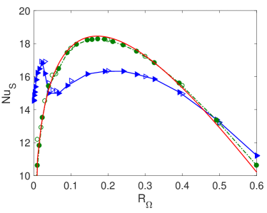
In one conjectured asymptotic regime of thermal convection (Spiegel, 1963) it is expected that $\alpha={1}/{2}$ so that the maximal momentum transport would occur for $\mbox{R}_{\Omega,m}\sim{1}/{4}$. The Reynolds numbers in numerical simulations and even in experiments are not high enough to reach this regime, and one resorts to Reynolds number dependent local scaling exponents. For RPC and $\Rey_{S}=2\times 10^{4}$, Salewski & Eckhardt (2015) find a maximum near $\mbox{R}_{\Omega,m}\approx 0.2$. The transition from TCF to RPC is discussed in Brauckmann et al. (2016), where it is shown that the maximum again appears near $\mbox{R}_{\Omega,m}\approx 0.2$ when the ratio of the radius of the inner cylinder to that of the outer cylinder is $0.99$. This observation is further cemented by the recent numerical and experimental results reported in Ezeta et al. (2020). Both sets of data (for TCF and RPC) are shown in Figure 2 (blue symbols). This agreement with observations is remarkable because the derivation here is valid only for the 2D setting with a rescaling of $v$ that violates the natural scaling of the velocity fields, whereas the reported maxima of $\textrm{R}_{\Omega}\sim 0.2$ comes from numerical studies of the full 3D flow. However, since rotation reduces the transverse components and enhances the azimuthally invariant parts, Brauckmann et al. (2016) also isolated the contribution of the azimuthally invariant 2D component of the flow, shown in Figure 2 as the green data points. They show a maximum near $R_{\Omega}\approx 0.18$. Moreover, a fit of the 2D contributions to the functional form (14) with $\alpha=0.26$ approximates the data very well over essentially the entire range $0<R_{\Omega}<0.6$ for which data is available. This confirms that the 2D analysis presented here can also explain features of the three-dimensional flow.

In turbulent RBC flows one expects the temperature to be well mixed in the interior, so that the profile consists, to a good approximation, of steep boundary layers near the top and bottom plates, and a region of constant temperature in the middle. We anticipate the same behavior will hold for the azimuthal velocity $v$ relative to the ${x}_{3}$ direction. Moreover, since equation (1c) is an explicit advection-diffusion equation, the temperature satisfies a maximum principle, i.e. ${T}$ is bounded by its values at the walls,

$$T_{0}\leq{T}\leq T_{0}+\delta T,$$

(16)

at any point in the volume. This arises because near a maximum the first derivative vanishes and the second is negative, so diffusion will act to reduce it. For RBC this indicates that there heat cannot pile up at the walls beyond that supplied by the boundary condition. Translated to RPC, the corresponding statement will address the relation between the downstream velocity and its value at the walls. A velocity field that lies outside the values provided by the boundary conditions is refered to in the literature as a backflow event. Existence of such backflow events has been a matter of controversy which was settled with the explicit demonstration of such events by Lenaers et al. (2012).

To see how the maximum principle applies to RPC, we let ${v}=-2\Omega{x}_{3}+\tilde{v}$, so that $\tilde{v}$ satisfies the advection diffusion equation ${\partial}_{t}\tilde{v}+({{\bf u}}\cdot{\nabla})\tilde{v}=\nu{\Delta}\tilde{v}$. This perturbative velocity field $\tilde{v}$ satisfies a maximum principle, i.e. its extreme values occur only at ${x}_{3}=0$ or ${x}_{3}=d$. This can be stated succinctly as $2\Omega d\leq\tilde{v}\leq U$, or $0\leq{v}\leq U$ for the original azimuthal velocity component (assuming a positive $U$). This implies that in this setting there is no backflow, i.e. the azimuthal velocity has a constant sign, and events like the ones observed by Lenaers et al. (2012) can not occur in 2D RPC. It would be of significant interest to determine if such events can occur for 3D RPC or even for the full TCF system. If so, one must question whether these events are present only for full three-dimensional flows or if the current restriction in RPC is unique.

Although the no-slip boundary condition is clearly the physically motivated choice for TCF, and hence for RPC as well, there is still some interest in considering the free-slip condition although there is less immediate physical motivation for this. Indeed, Rayleigh (1916) invoked free-slip conditions for mathematical convenience:

…for a further condition we should probably prefer $dw/dz=0$ [no-slip], corresponding to a fixed solid wall. But this entails much complication, and we may content ourselves with the supposition $d^{2}w/dz^{2}=0$ [free-slip]…

Thus, in the interest of reducing such complication due to the no-slip condition, we will consider stress-free (free-slip) boundary conditions on the plates for $u$ and $w$. As mentioned previously this is presented in the form $w=0$ and $\partial_{3}u=0$ at $x_{3}=0$ and $1$. Incompressibility then implies that the vorticity in the $x_{2}$ direction defined by $\omega_{2}=\partial_{1}w-\partial_{3}u$ vanishes at these boundaries as well. This leads to an enstrophy balance, where the enstrophy is defined as the square of the L² norm of $\omega_{2}$, i.e. $\|\omega_{2}\|_{2}^{2}$. This restriction which we consider in this Section only, does not reflect on any other aspect of the system as described above.

As shown by Whitehead & Doering (2011) this enstrophy balance, coupled with a uniform bound on $w(x_{3})$ near the boundary and a piece-wise linear, monotonic temperature profile, will yield a bound on the Nusselt number in RB of the form $\textrm{Nu}_{T}\leq c\textrm{Ra}^{5/12}$. Translated into the RPC system, this becomes

$$\textrm{Nu}_{S}\lesssim R_{\Omega}+\textrm{Re}_{S}^{5/6}(1-R_{\Omega})^{17/12}R_{\Omega}^{5/12},$$

(17)

which will have a maximum as $\textrm{Re}_{S}\rightarrow\infty$ for $\mbox{R}_{\Omega,m}=\frac{5}{22}\sim 0.227$ by equation (15). This is the only setting to date for which the scaling of $\textrm{Nu}_{S}$ is sublinear with respect to $\textrm{Re}_{S}$, deviating from the anticipated $\textrm{Re}_{S}^{1}$ scaling. Remarkably this scaling affects the $\textrm{Re}_{S}$-dependence, but it has little influence on the location of the maxima in $\textrm{R}_{\Omega}$.

References

- Ahlers & Behringer (1978) Ahlers, G. & Behringer, R.P. 1978 Evolution of turbulence from rayleigh-bénard instability. Physical Review Letters 40 (11), 712–716.
- Bradshaw (1969) Bradshaw, P. 1969 The analogy between streamline curvature and buoyancy in turbulent shear flow. Journal of Fluid Mechanics 36, 177–191.
- Brauckmann et al. (2017) Brauckmann, Hannes J., Eckhardt, Bruno & Schumacher, Jörg 2017 Heat transport in Rayleigh-Bénard convection and angular momentum transport in Taylor-Couette flow: a comparative study. Philosophical Transactions A 375 (2089).
- Brauckmann et al. (2016) Brauckmann, Hannes J, Salewski, Matthew & Eckhardt, Bruno 2016 Momentum transport in Taylor–Couette flow with vanishing curvature. Journal of Fluid Mechanics 790, 419–452.
- Busse (1969) Busse, F. H. 1969 Bounds on transport of mass and momentum by turbulent flow between parallel plates. Zeitschrift für Angewandte Mathematik und Physik 20 (1), 1–14.
- Chandrasekhar (1961) Chandrasekhar, S. 1961 Hydrodynamics and hydro-magnetic stability. Clarendon Press, Oxford, UK.
- Chossat & Iooss (2012) Chossat, P & Iooss, G 2012 The Couette-Taylor Problem. Springer New York.
- Constantin (1994) Constantin, P. 1994 Geometric statistics in turbulence. SIAM Review 36 (1), 73–98.
- Doering & Constantin (1992) Doering, C. R. & Constantin, P. 1992 Energy dissipation in shear driven turbulence. Physical Review Letters 69 (11), 1648–1651.
- Doering & Constantin (1994) Doering, C. R. & Constantin, P. 1994 Variational bounds on energy dissipation in incompressible flows: Shear flow. Physical Review E. 49, 4087–4099.
- Doering & Constantin (1996) Doering, C. R. & Constantin, P. 1996 Variational bounds on energy dissipation in incompressible flows. III. Convection. Physical Review E. 53 (6), 5957–5981.
- Doering et al. (2006) Doering, C. R., Otto, F. & Reznikoff, M. G. 2006 Bounds on vertical heat transport for infinite-Prandtl-number Rayleigh-Bénard convection. Journal of Fluid Mechanics 560, 229–241.
- Dubrulle & Hersant (2002) Dubrulle, B. & Hersant, F. 2002 Momentum transport and torque scaling in Taylor-Couette flow from an analogy with turbulent convection. European Physics Journal B 26, 379–386.
- Eckhardt et al. (2007a) Eckhardt, B., Grossmann, S. & Lohse, D. 2007a Fluxes and energy dissipation in thermal convection and shear flows. Europhysics Letters 78 (2), 7 pages.
- Eckhardt et al. (2007b) Eckhardt, B., Grossmann, S. & Lohse, D. 2007b Torque scaling in turbulent Taylor-Couette flow between independently rotating cylinders. Journal of Fluid Mechanics 581, 221–250.
- Ezeta et al. (2020) Ezeta, Rodrigo, Sacco, Francesco, Bakhuis, Dennis, Huisman, Sander G, Ostilla-Mónico, Rodolfo, Verzicco, Roberto, Sun, Chao & Lohse, Detlef 2020 Double maxima of angular momentum transport in tc turbulence. arXiv preprint arXiv:2006.03528 .
- Faisst & Eckhardt (2000) Faisst, Holger & Eckhardt, Bruno 2000 Transition from the Couette-Taylor system to the plane Couette system. Phys Rev E 61 (6 Pt B), 7227–7230.
- Gollub & Swinney (1975) Gollub, J. P. & Swinney, H. L. 1975 Onset of turbulence in a rotating fluid. Physical Review Letters 35 (14), 927–930.
- Howard (1963) Howard, L. N. 1963 Heat transport by turbulent convection. Journal of Fluid Mechanics 17 (3), 405–432.
- Howard (1972) Howard, L. N. 1972 Bounds on flow quantities. Annual Review of Fluid Mechanics 4, 473–494.
- Jeffreys (1928) Jeffreys, H. 1928 Some Cases of Instability in Fluid Motion. Proceedings of the Royal Society of London A 118, 195–208.
- Lenaers et al. (2012) Lenaers, Peter, Li, Qiang, Brethouwer, Geert, Schlatter, Philipp & Örlü, Ramis 2012 Rare backflow and extreme wall-normal velocity fluctuations in near-wall turbulence. Phys Fluids A 24 (3), 035110.
- Manneville (2010) Manneville, Paul 2010 Instabilities, Chaos and Turbulence. Imperial College Press.
- Nagata (1986) Nagata, Masato 1986 Bifurcations in Couette flow between almost corotating cylinders. Journal of Fluid Mechanics 169, 229–250.
- Nagata (2013) Nagata, Masato 2013 A note on the mirror-symmetric coherent structure in plane Couette flow. Journal of Fluid Mechanics 727, R1.
- Nickerson (1969) Nickerson, E. C. 1969 Upper bounds on torque in cylindrical couette flow. Journal of Fluid Mechanics 38 (4), 807–815.
- Otto & Seis (2011) Otto, F. & Seis, C. 2011 Rayleigh-Bénard convection: Improved bounds on the Nusselt number. Journal of Mathematical Physics 52, 083702.
- Plasting & Kerswell (2003) Plasting, S. C. & Kerswell, R. R. 2003 Improved upper bound on the energy dissipation rate in Plane Couette flow: the full solutions to Busse’s problem and the Constantin-Doering-Hopf problem with one-dimensional background fields. Journal of Fluid Mechanics 477, 363–379.
- Rayleigh (1916) Rayleigh, Lord 1916 On convection currents in a horizontal layer of fluid, when the higher temperature is on the under side. Philosophical Magazine and Journal of Science 32 (192), 529–546.
- Salewski & Eckhardt (2015) Salewski, Matthew & Eckhardt, Bruno 2015 Turbulent states in plane Couette flow with rotation. Phys Fluids A 27 (4), 045109.
- Spiegel (1963) Spiegel, E. A. 1963 A generalization of the mixing-length theory of thermal convection. Astrophysical Journal 138, 216–225.
- Veronis (1970) Veronis, George 1970 The Analogy Between Rotating and Stratified Fluids. Annu Rev Fluid Mech 2, 37–66.
- Whitehead & Doering (2011) Whitehead, J. P. & Doering, C. R. 2011 The ultimate regime of two-dimensional Rayleigh-Bénard convection with stress-free boundaries. Physical Review Letters 106, 244501.
- Whitehead & Doering (2012) Whitehead, J. P. & Doering, C. R. 2012 Rigid rigorous bounds on heat transport in a slippery container. Journal of Fluid Mechanics 707, 241–259.