Exact solutions for a spin-orbit coupled bosonic double-well system
Abstract
Exact solutions for spin-orbit (SO) coupled cold atomic systems are very important and rare in physics. In this paper, we propose a simple method of combined modulations to generate the analytic exact solutions for an SO-coupled boson held in a driven double well. For the cases of synchronous combined modulations and the spin-conserving tunneling, we obtain the general analytical accurate solutions of the system respectively. For the case of spin-flipping tunneling under asynchronous combined modulations, we get the special exact solutions in simple form when the driving parameters satisfy certain conditions. Based on these obtained exact solutions, we reveal some intriguing quantum spin dynamical phenomena, for instance, the arbitrary population transfer (APT) with and/or without spin-flipping, the controlled coherent population conservation (CCPC), and the controlled coherent population inversion (CCPI). The results may have potential applications in the preparation of accurate quantum entangled states and quantum information processing.
I Introduction
Exact solutions have played a central role in many branches of physicsbarnes109 , due to the fact that they not only can supplement numerical simulations, but also can deepen understanding of the underlying physicsZakrzewski32 . Therefore, since the birth of quantum mechanics, the search for exact solutions of quantum systems has been ongoingbarnes109 . Although widely studied over the past few decades, up to now many accurate solutions are obtained, which are based on two-level (or two-state) systemsbarnes109 ; Zakrzewski32 ; landau2 ; zener137 ; rosen40 ; rabi51 ; hioe32 ; hioe30 ; hai87 ; luoxb95 ; xie82 ; vitanov9 ; JC51 , such as the paradigmatic Landau-Zenerlandau2 ; zener137 and Rabirabi51 models, driven two-level systemsbarnes109 ; xie82 , complete population inversion by a phase jump for a two-state systemvitanov9 , the Jaynes-Cummings modelJC51 , and so on. The accurate analytic solution has proved to be very important in the contexts of qubit controlgre5 ; poem107 ; hai29 and has been extended to a series of precise controlsZakrzewski32 ; hioe30 ; hai87 ; luoxb95 ; xie82 ; vitanov9 ; bambini23 ; kyo71 ; gang82 . Not only that, the accurate solutions are extremely useful for the fundamental importance of quantum systems. However, for quantum systems with more levels, the exact solutions are more difficult to handle and are still lackingbere ; llorente .
In recent years, the study of spin-orbit (SO) coupling has been a hot topic, which has led to a number of interesting physical phenomenakato306 ; bernevig314 ; zutic76 ; step93 . It is found that SO coupling is specially appropriate for qubit control in the spintronic deviceszutic76 ; step93 ; flindt97 ; bednarek101 and plays a crucial role in topological quantum computingnayak80 . Synthetic SO coupling of both Bose and Fermi gases has been realized in recent experimentslin471 ; wang109 ; cheuk109 ; zhang109 ; huang12 ; wu354 ; zhang128 , which opens a completely new and ideal avenue for investigating quantum dynamics of SO-coupled cold atomic systems. There have been a great number of research works focusing on novel dynamics of SO-coupled cold atomic systemskart117 ; zhang628 ; tang121 ; wu99 ; ng92 ; zhang609 ; garcia89 ; citro224 ; tang ; cheng89 ; qu19 ; orso118 ; chen86 ; hu93 ; olson90 ; zcw108 ; yu90 ; ji99 ; luo93 ; luo52 ; luo22 ; gar114 ; abdu98 ; luo2021 ; luo39 ; luo74 , for instance, quantum spin dynamicstang121 ; wu99 , spin Josephson dynamicszhang609 ; garcia89 ; citro224 ; tang and localizationcheng89 ; qu19 , Anderson transition of SO-coupled cold atomsorso118 , collective dynamicszhang109 ; hu93 , Bloch oscillation dynamicsji99 , selective coherent spin transportationyu90 , spin-dependent dynamic localizationluo93 , controlling stable spin dynamicsluo22 , transparent manipulation of spin dynamicsluo39 , coherent control of spin tunnelingluo74 , and so on. To our knowledge, many works related to the quantum dynamics of SO-coupled cold atomic systems have been studied by applying approximate methodshu93 ; tang ; olson90 ; zcw108 ; ji99 ; cheng89 ; qu19 ; orso118 ; chen86 ; yu90 ; luo93 ; luo22 ; citro224 ; gar114 ; abdu98 ; luo52 ; luo2021 , for instance, numerical simulationhu93 ; olson90 ; zcw108 ; ji99 ; cheng89 ; qu19 ; orso118 , variational approximationhu93 ; cheng89 ; chen86 , mean-field approximationzcw108 , high-frequency approximation(or rotating-wave approximation)yu90 ; luo93 ; luo22 ; citro224 ; tang ; gar114 ; abdu98 ; luo39 ; luo74 , multiple-time-scale asymptotic analysisluo52 ; luo2021 , etc. However, the research on quantum spin dynamics of SO-coupled ultracold atomic systems based on exact solutions is still extremely rarehai29 .
In this paper, we present a simple method to construct the exact analytic solutions by applying combined modulations for an SO-coupled boson trapped in a double well potential (a four-level or four-state system). For the synchronous combined modulations case and the spin-conserving tunneling case, we obtain the analytical accurate solutions in general forms, respectively. For the spin-flipping case under asynchronous combined modulations, when the driving parameters are appropriately fixed, we get the simple particular exact solutions. Based on the obtained analytical exact solutions, some interesting quantum spin dynamical phenomena are revealed. Under synchronous combined modulations, the arbitrary population transfer (APT) with and/or without spin-flipping, the controlled coherent population conservation (CCPC), and the controlled coherent population inversion (CCPI) between left and right wells are shown. Under asynchronous combined modulations, for the spin-conserving and spin-flipping cases, we find new parametric conditions for performing the CCPC and CCPI, respectively. Our results may be useful for the preparation of precise quantum entangled states and the design of spintronic device.
II Model system
We consider an SO-coupled boson trapped in a driven double well, which is governed by the Hamiltonian
| (1) | |||||
Here and ( denotes the transpose). and are the creation and annihilation operators of a spin- () boson in the th () well respectively. is the effective strength of SO coupling and is the component of usual Pauli operator. represents the Hermitian conjugate of the preceding term. = denotes the number operator for spin in well , and are the time-dependent tunneling amplitude without SO coupling and Zeeman field, respectively. For simplicity, Eq. (1) has been treated as a dimensionless equation in which and the reference frequency (kHz is the single-photon recoil energy lin471 ) are set such that the parameters in and are in units of , and time is normalized in units of .
Employing the Fock basis to denote the state of a spin- boson occupying the right (left) well and no atom in the left (right) well, the quantum state of the SO-coupled bosonic system can be expanded as
| (2) |
where represents the time-dependent probability amplitude of the boson being in state or , for example, represents the time-dependent probability amplitude of the boson being in state . The occupation probability reads , which satisfies the normalization condition . For the convenience of studying dynamics, we define the population imbalance (, ) in which and are the total occupation populations of spin- boson in left and right wells respectively. Inserting Eqs. (1) and (2) into Schrödinger equation results in the coupled equations
Generally, it is very difficult to get the exact solution of Eq. (3), because of the different forms of the time-dependent modulation functions. Here, we will attempt to obtain the exact solution of Eq. (3) under the synchronous and asynchronous modulations, respectively.
III ANALYTICALLY EXACT SOLUTION UNDER THE SYNCHRONOUS MODULATIONS
For the synchronous modulations, we mean that the time-dependent driving functions and obey the relation hai87 , in which is a proportional constant. In such a case, by introducing a new time variable , Eq. (3) reduces to
| (4) |
which is the linear differential equations of with constant coefficients. In order to obtain the solutions of Eq. (4), we introduce the stationary solutions, , , , , where , , , and are constants obeying the normalization condition , and is the characteristic value. Inserting the stationary solutions into Eq. (4), we obtain the four characteristic values and the corresponding constants , , , for as
| (5) |
with constants , . Based on Eq. (5), we immediately get the four accurate stationary-like solutions (states) of the system
| (6) | |||||
for , which are the exact incoherent destruction of tunneling (IDT) states.
According to the superposition principle of quantum mechanics, we readily obtain the general exact solution of Eq. (4) by employing Eq. (6) to the linear superposition as
| (7) |
Here, for is an arbitrary superposition coefficient determined by the initial condition and normalization. Compared Eq. (7) with Eq. (2), the probability amplitudes are renormalized as
| (8) |
which is the general exact solution of Eq. (3) under the synchronous modulations. Obviously, any of the synchronous combined modulation functions and will generate an exact analytical solution to the Schrödinger equation, which thus enables us to produce an infinite variety of analytically exact solution (8) for the SO-coupled bosonic system. Here, we will select a square sech-shaped (a pulse-shaped) modulation function as an example to study the precise control of quantum spin dynamics by applying the exact solution under the synchronous modulations for the SO-coupled bosonic double-well system.
Let the modulation function sech2, where and are the driving strength and inverse pulse width respectivelyhai87 , such that the new time variable . Next, we will mainly discuss the APT with and/or without spin-flipping, the CCPC, and the CCPI between left and right wells based on the general exact solution (8).
III.0.1 APT with and/or without spin-flipping
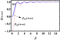
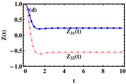
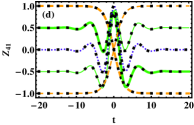
From the general exact solution (8), it is easily found that the population imbalance is a constant at and . Assuming the initial state of the system to be state with and , and according to the general exact solution (8), we plot the asymptotic population imbalances and as functions of the proportionality constant , the ratio of the driving strength and inverse pulse width , and the SO coupling strength shown in Figs. 1(a)-(c), respectively. In Fig. 1(a), the parameters are taken as (), , and . In this case, only quantum tunneling with spin-flipping can occur. Therefore, is equal to . It is easily seen from Fig. 1(a) that the asymptotic population imbalance can be continuously changed in the regime by adjusting the proportionality constant , which means the APT with spin-flipping (or the APT between state and state ) can be realized. To confirm our result, we select in Fig. 1(a) as an example to plot the time evolutions of the population imbalances (see Fig. 1(d)). From Fig. 1(d), one can get and which are in agreement with the results shown in Fig. 1(a). Furthermore, we find that as the proportionality constant increases, the asymptotic population imbalances and will tend to one in Fig. 1(a), which mean the coherent destruction of tunneling (CDT) happens (not shown here).
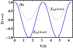
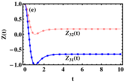
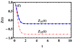
In Fig. 1(b), we set the parameters and (). Such that only quantum tunneling without spin-flipping can be performed and . The asymptotic population imbalance can be continuously adjusted in the regime via regulating the ratio value , which means the APT without spin-flipping (or the APT between state and state ) can be actualized. For example, we fix in Fig. 1(b) to plot the time evolutions of the population imbalances (see Fig. 1(e)). It can be seen from Fig. 1(e) that the asymptotic population imbalances and which are consistent with the results shown in Fig. 1(b). Specially, when in Fig. 1(b), the asymptotic population imbalance which means the completely tunneling without spin-flipping from the initial state to the final state takes place (not shown here).
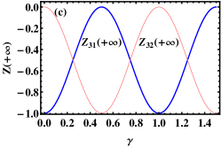
In Fig. 1(c), the parameters , , and are fixed. According to Eq. (8) and normalization condition, one can get , , and . It is obviously seen from Fig. 1(c) that the asymptotic population imbalances and oscillate periodically with the SO coupling strength in the region , which mean the tunneling probabilities with and without spin-flipping can be controlled, namely, the APT with and without spin-flipping can be manipulated. As an example, we take in Fig. 1(c) to plot the time evolutions of the population imbalances (see Fig. 1(f)). In Fig. 1(f), the asymptotic population imbalances and that are accordant with the results shown in Fig. 1(c). In particular, when , which means the spin-flipping and spin-conserving quantum tunneling with equal probability will simultaneously happen (not shown here).
III.0.2 CCPC and CCPI between left and right wells
Now, we mainly discuss the CCPC and CCPI between left and right wells. From the exact solution (8), we surprisingly find that when the parameters satisfy
| (9) |
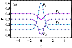
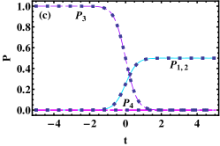
the probability () which means the final occupation probability of particle returns to the initial occupation probability as time goes from to and the final state is controllable. Thus, we call it CCPC. Here, we set the initial conditions , , , , and take the parameters , , , and to plot the time evolutions of the probabilities as shown in Fig. 2(a). From Fig. 2(a), one can find the probability , that is to say, the CCPC occurs. But, it is worth noting that the curves have oscillation around t=0, which imply the quantum transitions of particle between Fock states.
Further, from the accurate solution (8) we also notice that when the parameters satisfy
| (10) |
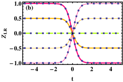
the population imbalances which mean the total populations in left well and that in right well inverse as time goes from to and the final populations in left and right wells can be controlled by setting appropriately initial conditions. So we call it CCPI between left and right wells. As an example, we take the same parameters as those of Fig. 2(a) except for and plot the time evolutions of the population imbalance for different initial conditions as shown in Fig. 2(b). It is obviously seen that . Therefore, the CCPI between left and right wells happens. That is to say, the CCPI still exists under the synchronous modulations in the SO-coupled bosonic system (four-level system), which generalizes the result obtained in the two-level system under asynchronous modulation (see Ref. hai87 ). Furthermore, what’s particularly interesting is that we find the number of oscillating peaks (valleys) of the probability and the population imbalance near in Figs. 2(a) and (b) are equal to the corresponding value of (e.g., peak for the curve of the probability near in Fig. 2(a)), except for the case of the initial population imbalance in Fig. 2(b). Not only that we also find when the initial condition is and the SO coupling strength () for the case of CCPI between left and right wells, the probabilities which mean the spin-flipping and spin-conserving tunneling with equal probability occurs simultaneously as shown in Fig. 2(c).
IV ANALYTICALLY EXACT SOLUTIONS UNDER THE ASYNCHRONOUS MODULATIONS
In this section, by using the tanh-shaped modulation and sech-shaped modulation = sech, our aim is to get the exact solutions of the asynchronous modulation system for the cases of spin-conserving and spin-flipping tunneling respectively. Then, applying those exact solutions to study the CCPC and CCPI with or without spin-flipping. From Eq. (3), it can be seen that when , is only coupled with and is only coupled with , which mean only the quantum tunneling without spin-flipping can occur. In order to investigate the exact CCPC and CCPI without spin-flipping, without loss of generality, we set (e.g., ), such that Eq. (3) reduces to two set of decoupled subequations as
| (11a) | ||||
| (11b) | ||||
Here, we solve Eq. (11a) as an example. By introducing the transformation and and inserting them to Eq. (11a), such that the Eq. (11a) reduces to
| (12) |
By using a time scale, , and utilizing the relation , the Eq. (12) can be simplified to the form
| (13) |
Obviously, the general solution of Eq. (13) can be easily obtained as
| (14) |
Such that we can get the exact solution of Eq. (11a) as
| (15) |
Similarly, we can obtain the precise solution of Eq. (11b) as
| (16) |
Here, the complex superposition constants and are determined by the initial conditions and normalization respectively.
These solutions, Eqs. (15) and (16), are the exact ones corresponding for the case of spin-conserving tunneling for arbitrary modulation functions and . Here, we only consider the asynchronous modulations and = sech. In such case, from Eq.(15), we surprisingly find when the parameters satisfy
| (17) |
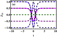
the populations and with the population imbalances (here, sign corresponds to respectively), which mean the CCPC occurs as time goes from to . As an example, we take the parameters , , , and set the different initial conditions to plot the time evolutions of the population imbalance in Fig. 3 (a). It can be seen that for different initial conditions the population imbalances remain unchanged as , namely, the CCPC happens.
When the parameters satisfy
| (18) |
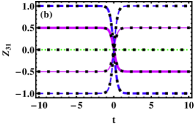
the populations and with the population imbalances (here, sign corresponds to respectively), which mean the occurrence of CCPI without spin-flipping as time . As an example, we take the same parameters and initial conditions as those of Fig. 3(a), except for , and plot the time evolutions of the population imbalance in Fig. 3 (b). It can be seen that the population imbalance under the different initial conditions, which means the CCPI occurs.
It is worth noting that the time-evolution curves of the population imbalance have oscillation around and the number of oscillating peak (or valley) for each curve is equal to the value and in Figs. 3(a) and (b) respectively, e.g., in Fig. 3(a) and in Fig. 3(b). Specially, when the initial population imbalance , the population of particle will keep standstill which means the occurrence of CDT, see Figs. 3(a) and (b). The analytical results (the squares) from Eq. (15) are in complete agreement with the numerical results (the curves) from Eq. (11a). For the exact solution (16), we can obtain the similar results.
Next, we study the exact CCPI with spin-flipping and set in Eq. (3) which means only quantum tunneling with spin-flipping can occur. Without loss of generally, we fix (e.g., ), such that Eq. (3) reduces to two set of decoupled subequations as
| (19a) | ||||
| (19b) | ||||
Note that the Eqs. (19a) and (19b) are analogous to Eq. (3) in Ref. hai87 , so we use the established method in Ref. hai87 to solve Eq. (19a) as an example to show the exact CCPI with spin-flipping. Let and from Eq. (19a) we can obtain the second-order equation
| (20) |
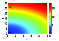
which is exactly solvable by the use of hypergeometric functionshai78 . Here, in order to get a simple solution, we select the driving parameters to satisfy
| (21) |
which is shown in Fig. 3(c). Based on Eq. (21), we can obtain the simple general solution of Eq. (20) as with constant determined by the initial condition. Such that the simple exact solution of Eq. (19a) is obtained as
It is worth noting that Eq. (22) implies and with the population imbalance , which mean the exact CCPI with spin-flipping can be implemented. As an example, we take the SO coupling strength and fix the parameters , and obeying Eq. (21) to plot the time evolutions of the population imbalance for the different initial conditions as shown in Fig. 3(d). It is obviously seen that the population imbalances , which mean the CCPI with spin-flipping happens. Here, we note that the time-evolution curve for the initial population imbalance has oscillation, which is different from the case of CCPI without spin-flipping (see Fig. 3(b)). The exact results (the squares) from Eq. (22) are in good agreement with the numerical results (the curves) from Eq. (19a).
By using the homologous method of solving Eq. (19a), we readily get the simple exact solution of Eq. (19b) as
| (23) |
where the constant is determined by the initial condition and the driving parameters must also obey Eq. (21). Likewise, it is also noticed in Eq. (23) that and with the population imbalance (not shown here). Note that the above results obtained in the case of spin-flipping are similar to ones obtained in the two-level system without SO coupling (see Ref. hai87 ), which goes against common intuition.
V CONCLUSION and DISCUSSION
In summary, we have proposed a simple method of combined modulations to obtain the analytical exact solutions for an SO-coupled boson trapped in a driven double-well potential. For the cases of synchronous combined modulations and the non-spin-flipping tunneling, we have obtained the general analytical precise solutions of the system respectively. For the spin-flipping tunneling case under asynchronous combined modulations, we have gotten the particular accurate solutions in simple form when the driving parameters are appropriately chosen. Based on these obtained accurate solutions, we have revealed some intriguing spin dynamical phenomena. Under synchronous combined modulations, the APT with and/or without spin-flipping, the CCPC, and the CCPI between left and right wells have been displayed. Under asynchronous combined modulations, we have also performed the CCPC and the CCPI with spin-conserving or with spin-flipping, respectively. Surprisingly, we have found that the CCPI exists in the cases of synchronous and asynchronous combined modulations in the SO-coupled cold atomic system (four-level system), which generalizes the result obtained in the case of asynchronous modulation in the two-level system without SO coupling (see Ref. hai87 ). The results may have potential applications in the qubit manipulation and the preparation of accurate quantum entangled states.
ACKNOWLEDGMENTS
This work was supported by the Hunan Provincial Natural Science Foundation of China under Grants No. 2021JJ30435 and No. 2017JJ3208, the Scientific Research Foundation of Hunan Provincial Education Department under Grants No. 21B0063 and No. 18C0027, and the National Natural Science Foundation of China under Grant No. 11747034.
References
- (1) E. Barnes and S. Das Sarma, Phys. Rev. Lett. 109, 060401 (2012).
- (2) J. Zakrzewski, Phys. Rev. A 32, 3748 (1985).
- (3) L. D. Landau, Physik Z. Sowjetunion 2, 46 (1932).
- (4) C. Zener, Proc. R. Soc. Lond. A 137, 696 (1932).
- (5) N. Rosen and C. Zener, Phys. Rev. 40, 502 (1932).
- (6) I. I. Rabi, Phys. Rev. 51, 652 (1937).
- (7) F. T. Hioe and C. E. Carroll, Phys. Rev. A 32, 1541 (1985).
- (8) F. T. Hioe, Phys. Rev. A 30, 2100 (1984).
- (9) W. Hai, K. Hai, and Q. Chen, Phys. Rev. A 87, 023403 (2013).
- (10) X. Luo, B. Yang, X. Zhang, L. Li, and X. Yu, Phys. Rev. A 95, 052128 (2017).
- (11) Q. Xie and W. Hai, Phys. Rev. A 82, 032117 (2010).
- (12) N. V. Vitanov, New J. Phys. 9, 58 (2007).
- (13) E. T. Jaynes and F. W. Cummings, Proc. IEEE 51, 89 (1963).
- (14) A. Greilich, S. E. Economou, S. Spatzek, D. R. Yakovlev, D. Reuter, A. D. Wieck, T. L. Reinecke, and M. Bayer, Nat. Phys. 5, 262 (2009).
- (15) E. Poem, O. Kenneth, Y. Kodriano, Y. Benny. S. Khatsevich, J. E. Avron, and D. Gershoni, Phys. Rev. Lett. 107, 087401 (2011).
- (16) K. Hai, W. Zhu, Q. Chen, and W. Hai, Chin. Phys. B 29, 083203 (2020).
- (17) A. Bambini and P. R. Berman, Phys. Rev. A 23, 2496 (1981).
- (18) E. S. Kyoseva and N. V. Vitanov, Phys. Rev. A 71, 054102 (2005).
- (19) A. Gangopadhyay, M. Dzero, and V. Galitski, Phys. Rev. B 82, 024303 (2010).
- (20) V. P. Berezovoj, M. I. Konchatnij, and A. J. Nurmagambetov, J. Phys. A: Math. Theor. 46, 065302 (2013).
- (21) J. M. G. Llorente and J. Plata, Phys. Rev. A 49, 2759 (1994).
- (22) Y. K. Kato, R. C. Myers, A. C. Gossard, and D. D. Awschalom, Science 306, 1910 (2004).
- (23) B. A. Bernevig, T. L. Hughes, and S. C. Zhang, Science 314, 1757 (2006).
- (24) I. Žutić, J. Fabian, and S. Das Sarma, Rev. Mod. Phys. 76, 323 (2004).
- (25) D. Stepanenko, N. E. Bonesteel, Phys. Rev. Lett. 93, 140501 (2004).
- (26) C. Flindt, A. S. Sørensen, K. Flensberg, Phys. Rev. Lett. 97, 240501 (2006).
- (27) S. Bednarek, B. Szafran, Phys. Rev. Lett. 101, 216805 (2008).
- (28) C. Nayak, S. H. Simon, A. Stern, M. Freedman, and S. Das Sarma, Rev. Mod. Phys. 80, 1083 (2008).
- (29) Y. Lin, K. Jiménez-García, and I. B. Spielman, Nature (London) 471, 83 (2011).
- (30) P. J. Wang, Z. Q. Yu, Z. K. Fu, J. Miao, L. H. Huang, S. J. Chai, H. Zhai, and J. Zhang, Phys. Rev. Lett. 109, 095301 (2012).
- (31) L. W. Cheuk, A. T. Sommer, Z. Hadzibabic, T. Yefsah, W. S. Bakr, and M. W. Zwierlein, Phys. Rev. Lett. 109, 095302 (2012).
- (32) J. Zhang, S. Ji, Z. Chen, L. Zhang, Z. Du, B. Yan, G. Pan, B. Zhao, Y. Deng, H. Zhai, S. Chen, and J. Pan, Phys. Rev. Lett. 109, 115301 (2012).
- (33) L. Huang, Z. Meng, P. Wang, P. Peng, S. L. Zhang, L. Chen, D. Li, Q. Zhou, and J. Zhang, Nat. Phys. 12, 540 (2016).
- (34) Z. Wu, L. Zhang, W. Sun, X. T. Xu, B. Z. Wang, S. C. Ji, Y. Deng, S. Chen, X. J. Liu, and J. W. Pan, Science 354, 83 (2016).
- (35) S. Zhang and G. Jo, J. Phys. Chem. Solids 128, 75 (2019).
- (36) Y. V. Kartashov, V. V. Konotop, D. A. Zezyulin, and L. Torner, Phys. Rev. Lett. 117, 215301 (2016).
- (37) D. Zhang, Z. Xue, H. Yan, Z. Wang, and S. Zhu, Phys. Rev. A 85, 013628 (2012).
- (38) W. Tang and S. Zhang, Phys. Rev. Lett. 121, 120403 (2018).
- (39) C. Wu, J. Fan, G. Chen, and S. Jia, Phys. Rev. A 99, 013617 (2019).
- (40) H. T. Ng, Phys. Rev. A 92, 043634 (2015).
- (41) D. Zhang, L. Fu, Z. Wang, and S. Zhu, Phys. Rev. A 85, 043609 (2012).
- (42) M. A. Garcia-March, G. Mazzarella, L. Dell’Anna, B. Juliá-Díaz, L. Salasnich, and A. Polls, Phys. Rev. A 89, 063607 (2014).
- (43) R. Citro and A. Naddeo, Eur. Phys. J. Spec. Top. 224, 503 (2015).
- (44) J. Tang, Z. Hu, Z. Zeng, J. Xiao, L. Li, Y. Chen, A. Chen, and X. Luo, arXiv: 2208.13198 (2022).
- (45) Y. Cheng, G. Tang, and S. K. Adhikari, Phys. Rev. A 89, 063602 (2014).
- (46) C. Qu, L. P. Pitaevskii, and S. Stringari, New J. Phys. 19, 085006 (2017).
- (47) G. Orso, Phys. Rev. Lett. 118, 105301 (2017).
- (48) F. Hu, J. Wang, Z. Yu, A. Zhang, and J. Xue, Phys. Rev. E 93, 022214 (2016).
- (49) A. J. Olson, S. Wang, R. J. Niffenegger, C. Li, C. H. Greene, and Y. Chen, Phys. Rev. A 90, 013616 (2014).
- (50) Y. Zhang, L. Mao, and C. Zhang, Phys. Rev. Lett. 108, 035302 (2012).
- (51) W. Ji, K. Zhang, W. Zhang, and L. Zhou, Phys. Rev. A 99, 023604 (2019).
- (52) Z. Chen and H. Zhai, Phys. Rev. A 86, 041604(R) (2012).
- (53) X. Luo, Z. Zeng, Y. Guo, B. Yang, J. Xiao, L. Li, C. Kong, and A. Chen, Phys. Rev. A 103, 043315 (2021).
- (54) X. Luo, B. Yang, J. Cui, Y. Guo, L. Li, and Q. Hu, J. Phys. B: At. Mol. Opt. Phys. 52, 085301 (2019).
- (55) Z. Yu and J. Xue, Phys. Rev. A 90, 033618 (2014).
- (56) Y. Luo, G. Lu, C. Kong, and W. Hai, Phys. Rev. A 93, 043409 (2016).
- (57) Y. Luo, X. Wang, Y. Luo, Z. Zhou, Z. Zeng, and X. Luo, New J. Phys. 22, 093041 (2020).
- (58) K. Jiménez-García, L. J. Leblanc, R. A. Williams, M. C. Beeler, C. Qu, M. Gong, C. Zhang, and I. B. Spielman, Phys. Rev. Lett. 114, 125301 (2015).
- (59) F. Kh. Abdullaev and M. Salerno, Phys. Rev. A 98, 053606 (2018).
- (60) W. Li, H. Yin, J. Yi, Y. Luo, X. Xie, W. Hai, and Y. Luo, Results Phys. 39, 105706 (2022).
- (61) Y. Luo, J. Yi, W. Li, X. Xie, Y. Luo, and W. Hai, Commun. Theor. Phys. 74, 055104 (2022).
- (62) Y. Luo, G. Lu, J. Tan, and W. Hai, J. Phys. B: At. Mol. Opt. Phys. 48, 015002 (2015).
- (63) W. Hai, S. Rong, and Q. Zhu, Phys. Rev. E 78, 066214 (2008).