Examining the Robustness of Spiking Neural Networks on Non-ideal Memristive Crossbars

Abhiroop Bhattacharjee^∗, Youngeun Kim^∗, Abhishek Moitra, and Priyadarshini Panda ^∗ These authors have contributed equally to this work. Department of Electrical Engineering, Yale University, USA
{abhiroop.bhattacharjee, youngeun.kim, abhishek.moitra, priya.panda}@yale.edu

Abstract

Spiking Neural Networks (SNNs) have recently emerged as the low-power alternative to Artificial Neural Networks (ANNs) owing to their asynchronous, sparse, and binary information processing. To improve the energy-efficiency and throughput, SNNs can be implemented on memristive crossbars where Multiply-and-Accumulate (MAC) operations are realized in the analog domain using emerging Non-Volatile-Memory (NVM) devices. Despite the compatibility of SNNs with memristive crossbars, there is little attention to study on the effect of intrinsic crossbar non-idealities and stochasticity on the performance of SNNs. In this paper, we conduct a comprehensive analysis of the robustness of SNNs on non-ideal crossbars. We examine SNNs trained via learning algorithms such as, surrogate gradient and ANN-SNN conversion. Our results show that repetitive crossbar computations across multiple time-steps induce error accumulation, resulting in a huge performance drop during SNN inference. We further show that SNNs trained with a smaller number of time-steps achieve better accuracy when deployed on memristive crossbars.

Index Terms:

Spiking neural network, memristive crossbar, ANN-SNN conversion, energy-efficiency, non-idealities

I Introduction

The previous decade has witnessed the rise of Spiking Neural Networks (SNNs) in the context of low-power machine intelligence [1, 2]. SNNs, unlike Artificial Neural Networks (ANNs), process visual information with discrete binary spikes or events over multiple time-steps resulting in asynchronous event-driven processing. Recent works have shown that the event-driven behaviour of SNNs can be efficiently implemented on emerging neuromorphic hardware to yield 1-2 orders of magnitude of energy-efficiency compared to that of ANNs on static image classification problems [3, 4, 5]. To this end, memristive crossbars, built using Non-Volatile-Memory (NVM) devices, have emerged as a fast, compact and energy-efficient solution to implementing neural networks for In-Memory Computing (IMC) in the analog domain [6, 7].

Refer to caption — Figure 1: (a) Ideal crossbar with input voltages $V_{i}$ , synaptic conductances $G_{ij}$ and output currents $I_{j}=\sum_{i}{G_{ij}V_{i}}$ ; (b) Non-ideal crossbar with the interconnect and synaptic non-idealities annotated.

However, there are several pitfalls to IMC using analog crossbars. Crossbars possess several non-idealities such as, interconnect parasitics, non-linearities/variations in the synapses, etc. [8, 9] that result in imprecise dot-product currents, leading to performance (accuracy) degradation upon mapping neural networks. Many works have modelled these non-idealities to study their impact on the performance and robustness of crossbar-mapped ANNs [10, 11, 12, 13, 14]. Although SNNs, as compared to ANNs, have been shown to be more robust to input noise owing to inherent stochasticity in the spike-encoding methods [15], there is no work that assesses the impact of crossbar non-idealities on the performance (robustness) of SNN models. To this end, our work is aimed at understanding- How robust is an SNN, evaluated over multiple time-steps, with respect to its ANN counterpart when mapped onto non-ideal IMC crossbars? Our findings indicate that, for an SNN trained with gradient backpropagation, repetitive crossbar operations across multiple time-steps induce error accumulation due to non-idealities that has detrimental impact on the performance of SNNs on crossbars as compared to ANNs. On the other hand, an SNN converted from pre-trained ANN is not affected by the number of time-steps since the converted SNN is the approximated version of the ANN model.

In summary, the key contributions of this work are as follows:

•

This work for the first time compares the robustness of SNNs on non-ideal memristive crossbars against corresponding ANN models. We examine SNNs trained from various learning algorithms such as, Surrogate Gradient (SG) learning [16], ANN-SNN conversion [17], and Batch Normalization Through Time (BNTT) [18].
•

We conduct experiments with VGG5 and VGG9 network architectures for ANNs and SNNs using benchmark datasets, namely MNIST and CIFAR10, to show that SNNs underperform with respect to ANNs when mapped on non-ideal crossbars of size 64 $\times$ 64 and 32 $\times$ 32.
•

We also perform ablation studies using SG-trained VGG9/CIFAR10 SNNs with different time-steps (10, 20 and 30). We find that a reduction in the number of time-steps improves the performance of SNNs on non-ideal crossbars.
•

We introduce noise-aware batch normalization adaptation technique to mitigate the vulnerability of BNTT-trained SNNs on non-ideal crossbars.

II Related Works

There has been a plethora of works that have proposed hardware accelerator designs to carry out SNN inference showing a high degree of parallelism, throughput, and energy-efficiency [1, 19, 7, 3, 20, 5]. These include inference accelerators with a fully-digital architecture, such as IBM’s TrueNorth processor [5], as well one in which synaptic computational cores comprise of analog memristive crossbars, such as RESPARC [7]. A recent work [20] proposed a methodology to map spiking neurons on analog crossbar architectures such that neurons having higher spike activities are placed close together to reduce communication energy overheads and better energy-efficiency. In summary, the primary focus of majority of these works has been to facilitate sparse event-driven spike communications with the key objective of improving the energy-efficiency of the deployed SNNs. But, none of the works on crossbar-based accelerators for SNNs account for the impact of the inexorable parasitic non-idealities that can detrimentally impact the performance of the mapped SNN architectures. Unless it is ascertained that the trained SNN models can yield a descent performance on mapping onto non-ideal crossbar arrays, the energy-efficiency advantages extracted from SNNs become inconsequential.

There have been many prior works that have included non-idealities during the inference of ANNs on crossbars [12, 10, 21, 9, 11]. These include Crosssim [22] and Neurosim [23] platforms that include device-to-device variations in the NVM synapses during inference. However, the resistive crossbar non-idealities (interconnect parasitics) that lead to IR-drops during the dot-product operations are not modelled by these platforms. To this end, a recent work called RxNN [8] splits and maps an ANNs computations into crossbar operations and proposes a fast crossbar model (FCM) to accurately capture the impact of resistive crossbar non-idealities during inference. The non-ideality integration framework employed in this work for evaluating SNN models is similar to the RxNN method for ANNs, and can model the impact of both resistive and device-to-device non-idealities. With this framework, we conduct extensive experiments to show the community where the performance of SNNs on analog crossbars stands in comparison to their ANN counterparts.

III Background

III-A Memristive Crossbars and Non-Idealities

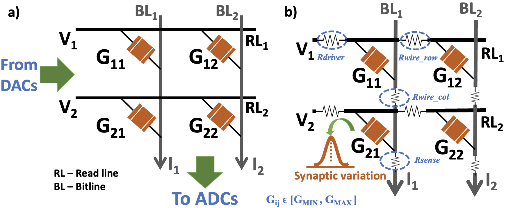
Memristive crossbars are used to realize Multiply-and-Accumulate (MAC) operations on IMC hardware in an analog manner. Crossbars receive the input activations of a neural network as analog voltages from Digital-to-Analog converters (DACs) and produce currents analogous to the outputs of MAC operations that are sensed by Analog-to-Digital converters (ADCs). Ideally, the MAC operations occur using Ohm’s Law and Kirchoff’s current law with the interaction of the input voltages and the memristive conductances for the synapses (programmed between $G_{MIN}$ and $G_{MAX}$ ) as shown in Fig. 1(a). However, the analog nature of the computation leads to various non-idealities, such as, circuit-level interconnect parasitics and synaptic-level non-linearities or variations [10, 9, 8].

Fig. 1(b) describes the equivalent circuit for a memristive crossbar consisting of various circuit-level and device-level non-idealities, viz. $Rdriver$ , $Rwire\_row$ , $Rwire\_col$ and $Rsense$ (interconnect parasitics), modelled as parasitic resistances and variations/non-linearities in the memristive synapses. The impact of these non-idealities or hardware noise can be incorporated by transforming the ideal memristive conductances $G_{ij(ideal)}$ (obtained from the weights of a neural network) to non-ideal conductances $G_{ij(non-ideal)}$ using linear algebraic operations and circuit laws. Consequently, the net output current sensed at the end of the crossbar-columns ( $I_{non-ideal}$ ) deviates from its ideal value ( $I_{ideal}$ ).

III-B Spiking Neural Networks

SNNs [1, 24] have gained attention due to their potential energy-efficiency compared to standard ANNs. The main feature of SNNs is the type of neural activation function for temporal signal processing, which is different from a ReLU activation for ANNs. A Leak-Integrate-and-Fire (LIF) neuron is commonly used as an activation function for SNNs. The LIF neuron $i$ has a membrane potential $u_{i}^{t}$ which accumulates the asynchronous spike inputs, which can be formulated as follows:

u_{i}^{t}=\lambda u_{i}^{t-1}+\sum_{j}w_{ij}o^{t}_{j}.

(1)

Here, $t$ stands for time-step, and $w_{ij}$ is for weight connections between neuron $i$ and neuron $j$ . Also, $\lambda$ is a leak factor. The LIF neuron $i$ accumulates membrane potential and generates a spike output $o_{i}^{t}$ whenever membrane potential exceeds the threshold $\theta$ :

o^{t}_{i}=\begin{cases}1,&\text{if $u_{i}^{t}>\theta$},\\ 0&\text{otherwise.}\end{cases}

(2)

The membrane potential is reset to zero after firing. This integrate-and-fire behavior of an LIF neuron generates a non-differentiable function, which is difficult to be used with standard backpropagation.

To address this, various training algorithms for SNNs have been studied in the past few decades. ANN-SNN conversion methods [17, 25, 26, 27, 28] convert pre-trained ANNs to SNNs using weight (or threshold) scaling in order to approximate ReLU activation with LIF activation. They can leverage well-established ANN training methods, resulting in high accuracy on complex datasets. On the other hand, surrogate gradient learning addresses the non-differentiability problem of a LIF neuron by approximating the backward gradient function [16]. Surrogate gradient learning can directly learn from the spikes, in a smaller number of time-steps. Based on the surrogate learning, several advanced algorithms have been proposed. Tandem learning [29, 30] designs an auxiliary ANN in order to stabilise error back-propagation for SNN training. Moreover, a line of work [31, 32] directly train membrane decay (or firing threshold) in an LIF neuron with standard weight update, resulting in a better representation power of SNNs. Batch Normalization (BN) technique [33] has been applied to accelerate the training process of SNNs [34, 18, 35]. In this work, we measure the impact of crossbar non-idealities during the inference of SNNs trained via both ANN-SNN conversion and surrogate gradients.

IV Robustness of SNNs on Memristive Crossbars

Algorithm 1 ANN-SNN Conversion [17]

Input: data set ( $X$ ); label set ( $Y$ ); max time-step ( $T$ ); network depth ( $L$ ); pre-trained ANN model ( $ANN$ ); SNN model ( $SNN$ )
Output: converted SNN network

SNN.weights\leftarrow ANN.weights

\triangleright

Copy weights

SNN.th

\leftarrow

\triangleright

Initialize firing threshold

3:for

l\leftarrow 1

L-1

4: for

t\leftarrow 1

T

O^{t}

\leftarrow

PoissonGenerator(X)

6: for

l^{\prime}\leftarrow 1

l

7: if

l^{\prime}<l

then

(O^{t}_{l},U_{l}^{t})\leftarrow(U_{l}^{t-1},W_{l},O^{t}_{l-1})

\triangleright

Forward (Eq. 1)

9: else

10:

SNN_{l}.th

\leftarrow

max(

SNN_{l}.th

{W_{l}O^{t}_{l-1}}

)

11: end if

12: end for

13: end for

14:end for

Algorithm 2 Training process with Surrogate Gradient

Input: data set ( $X$ ); label set ( $Y$ ); max time-step ( $T$ )
Output: updated network weights

1:for

i\leftarrow 1

max\_iter

2: fetch a mini batch X

3: for

t\leftarrow 1

T

4: O

\leftarrow

PoissonGenerator(X)

5: for

l\leftarrow 1

L-1

(O^{t}_{l},U_{l}^{t})\leftarrow(\lambda,U_{l}^{t-1},(W_{l},O^{t}_{l-1}))

7: end for

8: % For the final layer

L

, accumulate the voltage

U_{L}^{t}\leftarrow(U_{L}^{t-1},(W_{l},O^{t}_{L-1}))

10: end for

11: % Calculate the loss and back-propagation

12:

L\leftarrow(U_{L}^{T},Y)

13:end for

IV-A Optimizing SNNs

Here, we first describe two representative SNN training algorithms in detail used in our experiments.

ANN-SNN conversion: We use an iterative layer-wise ANN-SNN conversion method proposed in [17]. This method normalizes the firing thresholds in SNNs to approximate float activation value in a pre-trained ANN model. The overall conversion algorithm is presented in Algorithm 1. Firstly, we initialize SNNs using the weights from a pre-trained ANN (line 1). After that, we search the maximum activation value across all time-steps in a layer, and set the firing threshold with searched activation value (line 3-14). The conversion process starts from the first layer and sequentially goes through deeper layers.

TABLE I: Classification accuracy (%) of ANNs and SNNs on MNIST and CIFAR10 datasets. SW accuracy shows the clean performance achieved on a GPU machine. HW accuracy takes into account non-idealities in

64\times 64

crossbars during inference. The symbol

\Delta

represents a relative accuracy (performance) drop, i.e.,

\frac{SWaccuracy-HWaccuracy}{SWaccuracy}\times 100

, that denotes our metric to measure ANN and SNN performances.

Method	Architecture	Dataset	Time-steps	SW accuracy (%)	HW accuracy (%)	$\Delta$ (%)
ANN	VGG5	MNIST	-	99.34	99.20	0.14
ANN	VGG9	CIFAR10	-	91.90	86.29	6.10
Conversion [17]	VGG5	MNIST	50	99.26	99.07	0.19
Conversion [17]	VGG9	CIFAR10	500	91.02	86.40	5.07
Surrogate Gradient [16]	VGG5	MNIST	25	99.32	98.52	0.80
Surrogate Gradient [16]	VGG9	CIFAR10	30	86.70	14.94	82.76
BNTT [18]	VGG5	MNIST	10	99.45	11.35	88.58
BNTT [18]	VGG9	CIFAR10	20	90.43	10.01	88.93

Surrogate Gradient Backpropagation: Surrogate gradient learning approximates the non-differentiable firing behavior of LIF neurons by using surrogate function. Let $o^{t}_{i}$ and $u^{t}_{i}$ be output spikes and membrane potential at time-step $t$ of neuron $i$ , respectively. To calculate gradients, we use piece-wise linear backward function:

\frac{\partial o_{i}^{t}}{\partial u_{i}^{t}}=\max\{0,1-\ |\frac{u_{i}^{t}-\theta}{\theta}\ |\},

(3)

where, $\theta$ represents the firing threshold. With such an approximated function, surrogate gradient based backpropagation learning can be implemented on machine learning frameworks like PyTorch [36]. In our experiments, we use spatio-temporal back-propagation (STBP) [16]. They that accumulates the gradients over spatial and temporal dimensions which can be formulated as follows:

\frac{\partial L}{\partial W_{l}}=\begin{cases}\sum_{t}(\frac{\partial L}{\partial O_{l}^{t}}\frac{\partial O_{l}^{t}}{\partial U_{l}^{t}}+\frac{\partial L}{\partial U_{l}^{t+1}}\frac{\partial U_{l}^{t+1}}{\partial U_{l}^{t}})\frac{\partial U_{l}^{t}}{\partial W_{l}},&\text{if $l:$ hidden }\\ \frac{\partial L}{\partial U_{l}^{T}}\frac{\partial U_{l}^{T}}{\partial W_{l}}.&\text{if $l:$ output}\end{cases}

(4)

Here, $O^{t}_{l}$ and $U^{t}_{l}$ are output spikes and membrane potential at time-step $t$ for layer $l$ , respectively. The details are presented in Algorithm 2.

IV-B Experimental settings

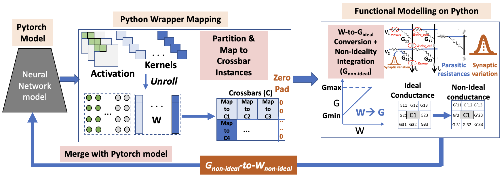
Hardware: In this work, we use a crossbar-based hardware evaluation framework (see Fig. 2) [13] to include the impact of crossbar non-idealities to the weights of a trained ANN or SNN during inference. The entire framework is written in Python. It involves a Python wrapper that reshapes the 4D convolutional weight-matrices of each layer of trained ANNs or SNNs into 2D matrices ( $W$ ) consisting of ideal weights. Thereafter, the matrices are partitioned into multiple crossbar instances (of a given size), followed by conversion of the ideal weights into synaptic conductances. Next, we model the resistive crossbar non-idealities using circuit laws and linear algebraic operations in Python [8] and obtain the non-ideal conductance matrices. Finally, the non-ideal synaptic conductances are transformed into non-ideal weights which are then integrated into the original Pytorch based ANN or SNN model to conduct inference. Note, we follow an NVM device agnostic approach for analyzing the impact of intrinsic circuit-level and synaptic crossbar non-idealities on the performance of SNNs or ANNs during inference. The ON/OFF ratio for the NVM devices in the crossbars is considered to be 10 (i.e., $R_{MIN}=20k\Omega$ and $R_{MAX}=200k\Omega$ ), typical for ReRAM devices. The resistive non-idealities (see Fig. 1(b)) are as follows: $Rdriver=1k\Omega$ , $Rwire\_row=5\Omega$ , $Rwire\_col=10\Omega$ and $Rsense=1k\Omega$ . The synaptic variations are modelled as a Gaussian variation in the synaptic conductances with $\sigma/\mu=10\%$ [10].

Software: In our experiments, we use two convolutional architectures (i.e., VGG5 and VGG9) on two public datasets (i.e., MNIST and CIFAR10). MNIST [37] contains gray-scale images of size 28 $\times$ 28. CIFAR10 [38] consists of 60,000 RGB color images of size 32 $\times$ 32 (50,000 for training / 10,000 for testing) with 10 categories. Our implementation is carried out on the PyTorch framework [36]. Total number of training epochs are set to 60 and 100 for MNIST and CIFAR10 datasets, respectively. During training, we utilize step-wise learning rate scheduling with a decay factor of 10 at 50% and 75% of the total epochs. We train the networks with Adam optimizer with an initial learning rate $1e-4$ .

TABLE II: Table with Classification accuracy (%) of ANNs and SNNs with VGG9 architecture on CIFAR10 dataset showing SW accuracy, HW accuracy and

\Delta

for 32

\times

32 and 64

\times

64 non-ideal crossbars during inference.

Method	Time-steps	Crossbar size	SW acc. (%)	HW acc. (%)	$\Delta$ (%)
ANN	-	32 $\times$ 32	91.90	90.46	1.56
ANN	-	64 $\times$ 64	91.90	86.29	6.10
Surrogate [16]	20	32 $\times$ 32	84.33	62.49	25.89
Surrogate [16]	20	64 $\times$ 64	84.33	14.21	83.14
BNTT [18]	20	32 $\times$ 32	90.43	10.01	88.93
BNTT [18]	20	64 $\times$ 64	90.43	10.01	88.93

IV-C Accuracy comparison with crossbar non-idealities

Table I shows the classification accuracies and performance ( $\Delta$ ) of ANNs and SNNs with the impact of crossbar non-idealities. From the experimental results, we observe the following: (1) ANN-SNN conversion shows similar performance with the corresponding ANN model since both are basically identical in nature and functionality. The converted SNN has the same weights and its spike rates across all the time-steps are proportional to the corresponding float ANN activations. (2) On the other hand, non-idealities bring a huge performance drop for surrogate gradient learning based SNNs as compared to ANNs. This is because surrogate gradient learning exploits spike dynamics (i.e., spike timing, membrane potential, etc) which are highly susceptible to crossbar non-idealities. Note, although surrogate gradient learning shows greater vulnerability on non-ideal crossbars, they can be implemented with a small number of time-steps. (3) As the dataset and network architecture gets more complicated, the performance drop increases. For instance, ANN, Conversion, and Surrogate gradient learning show less than $1\%$ accuracy drop on MNIST. However, for CIFAR10 dataset, the performance degradation increases significantly. (4) We also examine the effect of Batch Normalization (BN) technique for SNN, called BNTT [18], which presents temporal BN parameters. This technique enables SNNs to achieve high performance on software with even lesser number of time-steps. Note, BNTT is based on surrogate gradient learning. Our empirical results show that BNTT aggravates the computation error arising from crossbar non-idealities.

IV-D Ablation studies

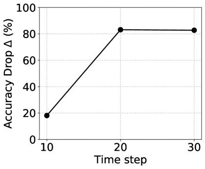
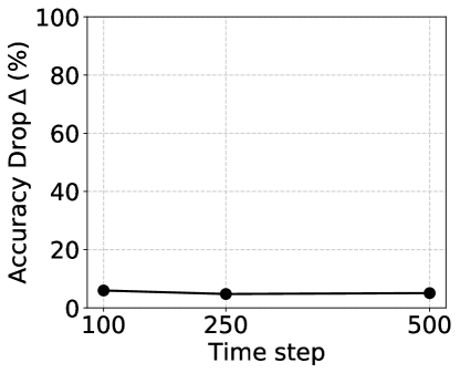
Time-steps: We explore the performance drop with respect to time-steps for the various SNN learning algorithms on $64\times 64$ non-ideal crossbars. In Fig. 3, we report the performance of surrogate gradient learning and ANN-SNN conversion with time-step {10, 20, 30} and {100, 250, 500}, respectively. For surrogate gradients, crossbar noise is accumulated across multiple time-steps, resulting in high performance drop at the high time-step regime. For the ANN-SNN conversion case, since the converted SNN can be approximated with the ANN model, the performance remains consistent irrespective of the number of time-steps.

Crossbar size: In addition to the previous experiments on $64\times 64$ crossbars, we evaluate the robustness of the SNN models on $32\times 32$ crossbars, having lesser non-idealities (see Table II). We find that for BNTT, a huge performance drop occurs for even smaller crossbar size of $32\times 32$ , while SG learning attains superior performance as compared to $64\times 64$ crossbars. This further validates the higher vulnerability of the BNTT-trained SNNs implemented on non-ideal crossbars. However, all performances are still inferior to the corresponding ANN models on comparing the $\Delta$ values for ANNs and SNNs in Table II).

IV-E Noise-aware BN adaptation for BNTT-trained SNNs

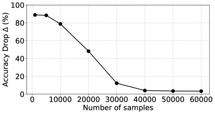
From Table I and Table II, we find that BNTT shows a huge performance degradation on crossbars owing to the distribution mismatch between clean and noisy activations. To address this, we present noise-aware BN adaptation which minimizes this mismatch by updating the average mean in the BN layers. Specifically, we forward a number of image samples through the SNN, adapting the moving average of BNTT with respect to noisy crossbar activations (while keeping other learnable parameters frozen). This can mitigate the impact of non-idealities on SNNs with BN techniques. Fig. 4 shows the variation of performance drop ( $\Delta$ ) with respect to the number of image samples forwarded during noise-aware BN adaptation. The results show that SNN performance drop decreases with increase in the number of image samples, and with a large number of samples can surpass the corresponding ANN performance on crossbars.

V Conclusion

We explore the impact of crossbar non-idealites on the performance of SNNs. Interestingly, we find that SNNs trained using surrogate gradient learning are more vulnerable to crossbar non-idealites compared to ANNs due to repetitive crossbar computations across multiple time-steps. This also leads to the finding that SNNs evaluated with a small number of time-steps show lower performance degradation on non-ideal crossbars. Furthermore, applying batch-normalization technique on SNNs amplifies the effect of non-idealites on the activations, thereby resulting in greater performance losses. Unless such vulnerabilities pertaining to SNNs are addressed, the seamless integration of the SNN algorithms with emerging NVM-based hardware architectures will be precarious. Thus, in future we will explore SNN-crafted training algorithms using noise-aware training [10] as well as managing the representation type/scheme of input spikes to crossbars [39], for mitigating the effect of non-idealites.

Acknowledgement

This work was supported in part by C-BRIC, a JUMP center sponsored by DARPA and SRC, the National Science Foundation (Grant#1947826), TII (Abu Dhabi) and the DARPA AI Exploration (AIE) program.

References

[1] K. Roy, A. Jaiswal, and P. Panda, “Towards spike-based machine intelligence with neuromorphic computing,” Nature, vol. 575, no. 7784, pp. 607–617, 2019.
[2] D. V. Christensen, R. Dittmann, B. Linares-Barranco, A. Sebastian, M. Le Gallo, A. Redaelli, S. Slesazeck, T. Mikolajick, S. Spiga, S. Menzel, et al., “2022 roadmap on neuromorphic computing and engineering,” Neuromorphic Computing and Engineering, 2022.
[3] M. Davies, N. Srinivasa, T.-H. Lin, G. Chinya, Y. Cao, S. H. Choday, G. Dimou, P. Joshi, N. Imam, S. Jain, et al., “Loihi: A neuromorphic manycore processor with on-chip learning,” Ieee Micro, vol. 38, no. 1, pp. 82–99, 2018.
[4] S. B. Furber, F. Galluppi, S. Temple, and L. A. Plana, “The spinnaker project,” Proceedings of the IEEE, vol. 102, no. 5, pp. 652–665, 2014.
[5] F. Akopyan, J. Sawada, A. Cassidy, R. Alvarez-Icaza, J. Arthur, P. Merolla, N. Imam, Y. Nakamura, P. Datta, G.-J. Nam, et al., “Truenorth: Design and tool flow of a 65 mw 1 million neuron programmable neurosynaptic chip,” IEEE transactions on computer-aided design of integrated circuits and systems, vol. 34, no. 10, pp. 1537–1557, 2015.
[6] I. Chakraborty, A. Jaiswal, A. Saha, S. Gupta, and K. Roy, “Pathways to efficient neuromorphic computing with non-volatile memory technologies,” Applied Physics Reviews, vol. 7, no. 2, p. 021308, 2020.
[7] A. Ankit, A. Sengupta, P. Panda, and K. Roy, “Resparc: A reconfigurable and energy-efficient architecture with memristive crossbars for deep spiking neural networks,” in Proceedings of the 54th Annual Design Automation Conference 2017, pp. 1–6, 2017.
[8] S. Jain, A. Sengupta, K. Roy, and A. Raghunathan, “Rxnn: A framework for evaluating deep neural networks on resistive crossbars,” IEEE Transactions on Computer-Aided Design of Integrated Circuits and Systems, vol. 40, no. 2, pp. 326–338, 2020.
[9] I. Chakraborty, M. F. Ali, D. E. Kim, A. Ankit, and K. Roy, “Geniex: A generalized approach to emulating non-ideality in memristive xbars using neural networks,” in 2020 57th ACM/IEEE Design Automation Conference (DAC), pp. 1–6, IEEE, 2020.
[10] A. Bhattacharjee, L. Bhatnagar, Y. Kim, and P. Panda, “Neat: Non-linearity aware training for accurate, energy-efficient and robust implementation of neural networks on 1t-1r crossbars,” IEEE Transactions on Computer-Aided Design of Integrated Circuits and Systems, 2021.
[11] B. Liu, H. Li, Y. Chen, X. Li, Q. Wu, and T. Huang, “Vortex: Variation-aware training for memristor x-bar,” in Proceedings of the 52nd Annual Design Automation Conference, pp. 1–6, 2015.
[12] A. Bhattacharjee, A. Moitra, and P. Panda, “Efficiency-driven hardware optimization for adversarially robust neural networks,” in 2021 Design, Automation & Test in Europe Conference & Exhibition (DATE), pp. 884–889, IEEE, 2021.
[13] A. Bhattacharjee and P. Panda, “Rethinking non-idealities in memristive crossbars for adversarial robustness in neural networks,” arXiv preprint arXiv:2008.11298, 2020.
[14] A. Bhattacharjee and P. Panda, “Switchx: Gmin-gmax switching for energy-efficient and robust implementation of binary neural networks on reram xbars,” 2021.
[15] S. Sharmin, N. Rathi, P. Panda, and K. Roy, “Inherent adversarial robustness of deep spiking neural networks: Effects of discrete input encoding and non-linear activations,” in European Conference on Computer Vision, pp. 399–414, Springer, 2020.
[16] Y. Wu, L. Deng, G. Li, J. Zhu, and L. Shi, “Spatio-temporal backpropagation for training high-performance spiking neural networks,” Frontiers in neuroscience, vol. 12, p. 331, 2018.
[17] A. Sengupta, Y. Ye, R. Wang, C. Liu, and K. Roy, “Going deeper in spiking neural networks: Vgg and residual architectures,” Frontiers in neuroscience, vol. 13, p. 95, 2019.
[18] Y. Kim and P. Panda, “Revisiting batch normalization for training low-latency deep spiking neural networks from scratch,” Frontiers in Neuroscience, 2021.
[19] P. Panda, S. A. Aketi, and K. Roy, “Toward scalable, efficient, and accurate deep spiking neural networks with backward residual connections, stochastic softmax, and hybridization,” Frontiers in Neuroscience, vol. 14, p. 653, 2020.
[20] A. Balaji, A. Das, Y. Wu, K. Huynh, F. G. Dell’Anna, G. Indiveri, J. L. Krichmar, N. D. Dutt, S. Schaafsma, and F. Catthoor, “Mapping spiking neural networks to neuromorphic hardware,” IEEE Transactions on Very Large Scale Integration (VLSI) Systems, vol. 28, no. 1, pp. 76–86, 2019.
[21] A. Bhattacharjee, L. Bhatnagar, and P. Panda, “Examining and mitigating the impact of crossbar non-idealities for accurate implementation of sparse deep neural networks,” 2022 Design, Automation & Test in Europe Conference & Exhibition (DATE), 2022.
[22] S. J. Plimpton, S. Agarwal, R. Schiek, and I. Richter, “Crosssim,” tech. rep., Sandia National Lab.(SNL-NM), Albuquerque, NM (United States), 2016.
[23] P.-Y. Chen, X. Peng, and S. Yu, “Neurosim: A circuit-level macro model for benchmarking neuro-inspired architectures in online learning,” IEEE Transactions on Computer-Aided Design of Integrated Circuits and Systems, vol. 37, no. 12, pp. 3067–3080, 2018.
[24] P. U. Diehl and M. Cook, “Unsupervised learning of digit recognition using spike-timing-dependent plasticity,” Frontiers in computational neuroscience, 2015.
[25] P. U. Diehl, D. Neil, J. Binas, M. Cook, S.-C. Liu, and M. Pfeiffer, “Fast-classifying, high-accuracy spiking deep networks through weight and threshold balancing,” in 2015 International joint conference on neural networks (IJCNN), pp. 1–8, ieee, 2015.
[26] B. Han and K. Roy, “Deep spiking neural network: Energy efficiency through time based coding,” in Computer Vision–ECCV 2020: 16th European Conference, Glasgow, UK, August 23–28, 2020, Proceedings, Part X 16, pp. 388–404, Springer, 2020.
[27] Y. Li, S. Deng, X. Dong, R. Gong, and S. Gu, “A free lunch from ann: Towards efficient, accurate spiking neural networks calibration,” arXiv preprint arXiv:2106.06984, 2021.
[28] B. Rueckauer, I.-A. Lungu, Y. Hu, M. Pfeiffer, and S.-C. Liu, “Conversion of continuous-valued deep networks to efficient event-driven networks for image classification,” Frontiers in neuroscience, vol. 11, p. 682, 2017.
[29] J. Wu, Y. Chua, M. Zhang, G. Li, H. Li, and K. C. Tan, “A tandem learning rule for effective training and rapid inference of deep spiking neural networks,” arXiv e-prints, pp. arXiv–1907, 2019.
[30] J. Wu, C. Xu, D. Zhou, H. Li, and K. C. Tan, “Progressive tandem learning for pattern recognition with deep spiking neural networks,” arXiv preprint arXiv:2007.01204, 2020.
[31] W. Fang, Z. Yu, Y. Chen, T. Masquelier, T. Huang, and Y. Tian, “Incorporating learnable membrane time constant to enhance learning of spiking neural networks,” in Proceedings of the IEEE/CVF International Conference on Computer Vision, pp. 2661–2671, 2021.
[32] N. Rathi and K. Roy, “Diet-snn: A low-latency spiking neural network with direct input encoding and leakage and threshold optimization,” IEEE Transactions on Neural Networks and Learning Systems, 2021.
[33] S. Ioffe and C. Szegedy, “Batch normalization: Accelerating deep network training by reducing internal covariate shift,” arXiv preprint arXiv:1502.03167, 2015.
[34] E. Ledinauskas, J. Ruseckas, A. Juršėnas, and G. Buračas, “Training deep spiking neural networks,” arXiv preprint arXiv:2006.04436, 2020.
[35] H. Zheng, Y. Wu, L. Deng, Y. Hu, and G. Li, “Going deeper with directly-trained larger spiking neural networks,” arXiv preprint arXiv:2011.05280, 2020.
[36] A. Paszke, S. Gross, S. Chintala, G. Chanan, E. Yang, Z. DeVito, Z. Lin, A. Desmaison, L. Antiga, and A. Lerer, “Automatic differentiation in pytorch,” 2017.
[37] Y. LeCun, L. Bottou, Y. Bengio, and P. Haffner, “Gradient-based learning applied to document recognition,” Proceedings of the IEEE, vol. 86, no. 11, pp. 2278–2324, 1998.
[38] A. Krizhevsky, G. Hinton, et al., “Learning multiple layers of features from tiny images,” 2009.
[39] Y. Kim, H. Kim, S. Kim, S. J. Kim, and P. Panda, “Gradient-based bit encoding optimization for noise-robust binary memristive crossbar,” arXiv preprint arXiv:2201.01479, 2022.


(a) Surrogate Gradients	(b) ANN-SNN Conversion