Excursions away from the Lipschitz minorant of a Lévy process
Abstract.
For , the -Lipschitz minorant of a function is the greatest function such that and for all , should such a function exist. If is a real-valued Lévy process that is not a pure linear drift with slope , then the sample paths of have an -Lipschitz minorant almost surely if and only if and . Denoting the minorant by , we consider the contact set , which, since it is regenerative and stationary, has the distribution of the closed range of some subordinator “made stationary” in a suitable sense. We provide a description of the excursions of the Lévy process away from its contact set similar to the one presented in Itô excursion theory. We study the distribution of the excursion on the special interval straddling zero. We also give an explicit path decomposition of the other “generic” excursions in the case of Brownian motion with drift with . Finally, we investigate the progressive enlargement of the Brownian filtration by the random time that is the first point of the contact set after zero.
Key words and phrases:
fluctuation theory, regenerative set, subordinator, last exit decomposition, global minimum, path decomposition, enlargement of filtration2010 Mathematics Subject Classification:
60G51, 60G55, 60J651. Introduction
Recall that a function is -Lipschitz for some if for all . Given a function , we say that dominates the -Lipschitz function if for all . A necessary and sufficient condition that dominates some -Lipschitz function is that is bounded below on compact intervals and satisfies and . When the function dominates some -Lipschitz function there is an -Lipschitz function dominated by such that for all for any -Lipschitz function dominated by ; we call the -Lipschitz minorant of . The -Lipschitz minorant is given concretely by
| (1.1) |
The purpose of the present paper is to continue the study of the -Lipschitz minorants of the sample paths of a two-sided Lévy process begun in [AE14].
A two-sided Lévy process is a real-valued stochastic process indexed by the real numbers that has càdlàg paths, stationary independent increments, and takes the value at time . The distribution of a two-sided Lévy process is characterized by the Lévy-Khintchine formula for and , where
with , , and a -finite measure concentrated on satisfying (see [Ber96, Sat99] for information about (one-sided) Lévy processes — the two-sided case involves only trivial modifications). In order to avoid having to consider annoying, but trivial, special cases in what follows, we henceforth assume that is not just deterministic linear drift , , for some ; that is, we assume that there is a non-trivial Brownian component () or a non-trivial jump component ().
The sample paths of have bounded variation almost surely if and only if and . In this case can be rewritten as
We call the drift coefficient.
We now recall a few facts about the -Lipschitz minorants of the sample paths of from [AE14].
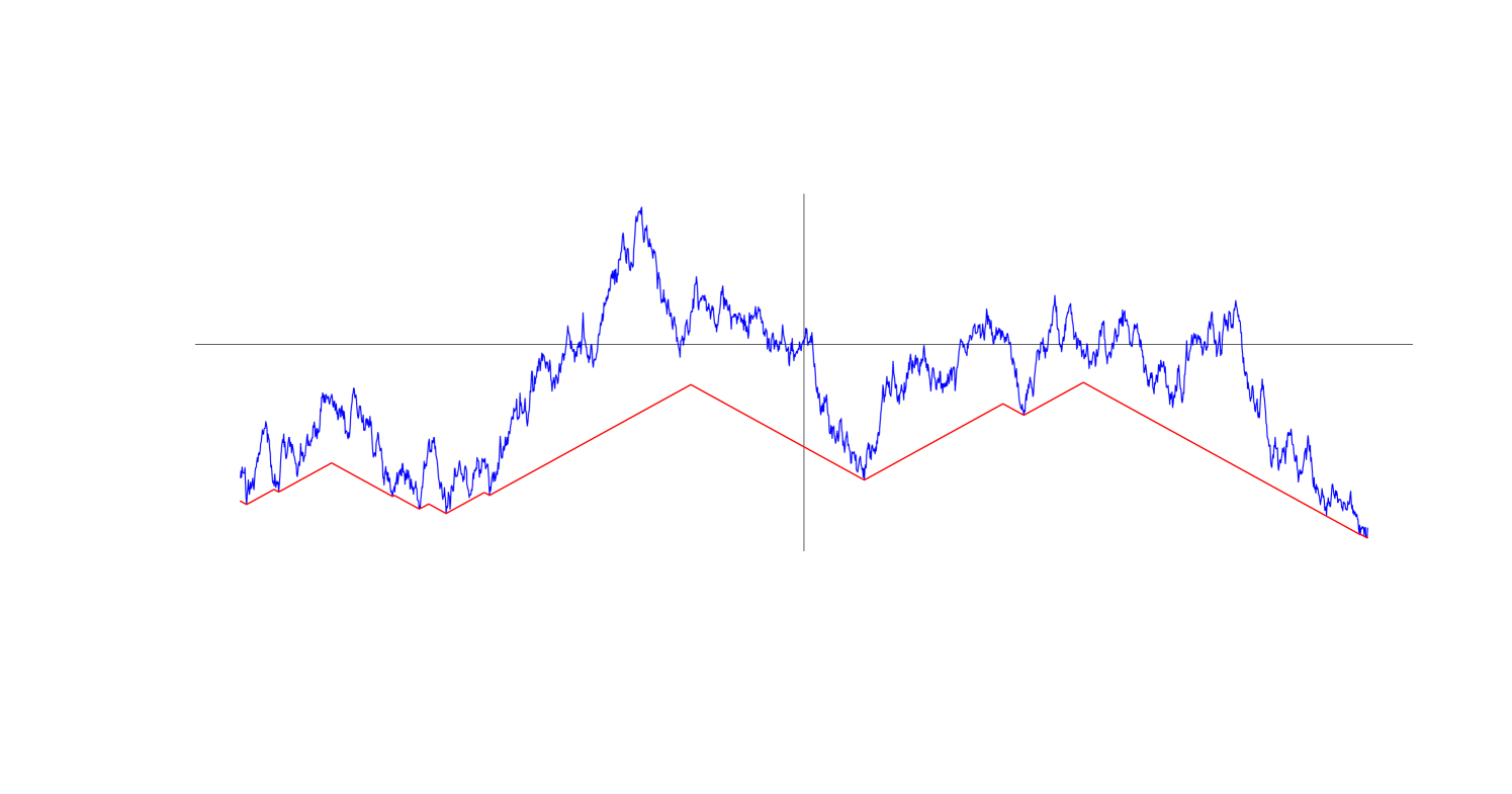
Either the -Lipschitz minorant exists for almost all sample paths of or it fails to exist for almost sample paths of . A necessary and sufficient condition for the -Lipschitz minorant to exist for almost all sample paths is that and . We assume from now on that this condition holds and denote the corresponding minorant process by . Figure 1.1 shows an example of a typical Brownian motion sample path and its associated -Lipschitz minorant.
Set . We call the contact set. The random closed set is non-empty, stationary, and regenerative in the sense of [FT88] (see Definition 2.1 below for a re-statement of the definition). Such a random closed set either has infinite Lebesgue measure almost surely or zero Lebesgue measure almost surely.
-
•
If the sample paths of have unbounded variation almost surely, then has zero Lebesgue measure almost surely.
-
•
If has sample paths of bounded variation and , then has zero Lebesgue measure almost surely.
-
•
If has sample paths of bounded variation and , then has infinite Lebesgue measure almost surely.
-
•
If has sample paths of bounded variation and , then whether the Lebesgue measure of is infinite or zero is determined by an integral condition involving the Lévy measure that we omit. In particular, if , , and , then the Lebesgue measure of is almost surely infinite.
If has zero Lebesgue measure, then is either almost surely a discrete set or almost surely a perfect set with empty interior.
-
•
If , then is almost surely discrete.
-
•
If and , then is almost surely discrete if and only if
-
•
If and , then is almost surely discrete if and only if .
The outline of the remainder of the paper is as follows.
In Section 2 we show that the pair is a space-time regenerative system in the sense that if for any , then is independent of with a distribution that does not depend on . It follows that if is discrete, we write for the successive positive elements of , and we set , , for the corresponding sequence of excursions away from the contact set, then these excursions are independent and identically distributed. When is not discrete there is a “local time” on and we give a description of the corresponding excursions away from the contact set as the points of a Poisson point process that is analogous to Itô’s description of the excursions of a Markov process away from a regular point.
Because is stationary, the key to establishing the space-time regenerative property is to show that if is the first positive point in , then is independent of . This is nontrivial because is most definitely not a stopping time for the canonical filtration of and so we can’t just apply the strong Markov property. We derive the claimed fact in Section 3 using a result from [Mil78] on the path decomposition of a real-valued Markov process at the time it achieves its global minimum. This result in turn is based on general last-exit decompositions from [PS72, GS74].
When the contact set is discrete we obtain some information about the excursion away from the -Lipschitz minorant that contains the time zero in Section 4 using ideas from [Tho00]. If is the last contact time before zero and , as above, is the first contact time after zero, we show that is independent of and uniformly distributed on . This observation allows us to describe the finite-dimensional distributions of in terms of those of , and we are able to determine the latter explicitly. The argument here is based on a generalization of the fact that if is a nonnegative random variable, is uniformly distributed on , and and are independent, then it is possible to express the distribution of in terms of that of .
As before, write , , for the independent, identically distributed sequence of excursions away from the contact set that occur at positive times in the case where the contact set is discrete. When is Brownian motion with drift , where in order for the -Lipschitz minorant to exist, we establish a path decomposition description for the common distribution of the in Section 5. Using this path decomposition we can determine the distributions of quantities such as the length and the distribution of the final value . Moreover, if we write for the excursion straddling time zero, then we have the “size-biasing” relationship , , for nonnegative measurable functions , and this allows us to recover information about the distribution of from a knowledge of the common distribution of the “generic” excursions , .
As we noted above, the random time is not a stopping time for the canonical filtration of . In Section 6 we investigate the filtration obtained by enlarging the Brownian filtration in such way that becomes a stopping time. Martingales for the Brownian filtration become semimartingales in the enlarged filtration and we are able to describe their canonical semimartingale decompositions quite explicitly.
2. Space-time regenerative systems
Let (resp. ) denote the space of càdlàg -valued paths indexed by (resp. ). For , define by
For define by
For , define by
Let (resp. ) denote the class of closed subsets of (resp. ). For define by
For define by
and by
With a slight abuse of notation, also use and , , to denote the analogously defined maps from to .
Put and . Define by
Define by
Finally, for define the following -fields on :
and
Define and analogously.
Definition 2.1.
Let (resp. ) be a probability measure on (resp. . Then is regenerative with regeneration law if
-
(i)
, for all ;
-
(ii)
for all and for all -measurable nonnegative functions ,
where we write and for expectations with respect to and .
Remark 2.2.
Suppose that the probability measure on is stationary; that is, that under the process has the same distribution as the process for all . Then, in order to check conditions (i) and (ii) of Definition 2.1, it suffices to check them for the case .
Theorem 2.3.
-
(i)
In order to check that the probability measure on is space-time regenerative with the probability measure on as regeneration law, it suffices to check
-
(a)
, for all ;
-
(b)
for all and for all -measurable nonnegative functions ,
-
(a)
-
(ii)
Suppose that the probability measure on is space-time regenerative with the probability measure on as regeneration law and that is an almost surely finite -stopping time. Then for all -measurable nonnegative functions
Proof.
(i) Fix . For set .
Consider of the form
for some and bounded, continuous function . For such an we have
for all and it suffices by a monotone class argument to show that
for all . This, however, is clear because and
by assumption.
(ii) For define a -stopping time by declaring that when , .
Let be as in the proof of part (i). For such an we have
for all and it suffices by a monotone class argument to show that
for all . Since for all , it further suffices to show that
Fix and suppose that is a nonnegative -measurable random variable. We have
where in the penultimate equality we used the fact that is -measurable (see, for example, [Kal02, Lemma 7.1(ii)]). This completes the proof. ∎
Theorem 2.4.
Suppose for the Lévy process that is regular for . Then the distribution of is space-time regenerative.
Remark 2.5.
If is not regular for for the Lévy process , then is regular for for the Lévy process . Equivalently, if is not regular for for the Lévy process , then is regular for for the Lévy process and hence for the Lévy process . Thus, either the distribution of is space-time regenerative or the distribution of is space-time regenerative.
Write for the projection . Define similarly. If is space-time regenerative with regeneration law , then, in the sense of [FT88], the push-forward of by is regenerative with regeneration law the push-forward of by . It follows that is either or .
Suppose that the probability in question is . Define -stopping times with almost surely by
and
where , , are the shift maps given by . Let be an isolated cemetery state adjoined to . Define càdlàg -valued processes , , by
where is the projection . Then, under , the sequence , , is independent and identically distributed.
The path of of each lies in the set consisting of càdlàg functions such that , , and for all .
When the probability in question is there is a local time on our regenerative set and we can construct a Poisson random measure on the set
that records the excursions away from the contact set and the order in which they occur. We use the following theorem which is a restatement of [GP80, Corollary 3.1].
Theorem 2.6.
Let be an increasing family of measurable sets in a measurable space such that . Let be an -valued point process; that is, is a stochastic process with values in for some adjoined point such that is almost surely countable. Suppose that is almost surely discrete and unbounded for all while is almost surely not discrete. Suppose that the sequence is independent and identically distributed for each . For define by setting for . For set and put . Then, for almost all , uniformly for bounded ,
where is continuous and nondecreasing in , and strictly increasing on . For such , set
Then is a homogeneous Poisson point process; that is, the random measure that puts mass at each point such that is a Poisson random measure with intensity of the form , where is Lebesgue measure on and is a -finite measure on . Moreover, for almost all for all with , .
We can apply this theorem if we consider to be the space of càdlàg paths that vanish at the origin and have finite lifetimes, and take to be the subspace of paths with lifetime at least . We define to be the point process of the excursions such that, for every , is equal to the excursion whose right end point is , with the convention that if is not the right end point of an excursion. In the case where is not discrete, all the conditions of Theorem 2.6 can readily be checked and we obtain a time-changed Poisson point process.
3. The process after the first positive point in the contact set
Notation 3.1.
For set and . Put and .
Remark 3.2.
Notation 3.3.
For put . Define the -field for any nonnegative random time to be the -field generated by all the random variables of the form where is an optional process with respect to the filtration . Similarly, define to be the -field generated by all the random variables of the form where is now a previsible process with respect to the filtration
Notation 3.4.
Let be a Hunt process such that the distribution of under is that of . Put , and for and put
We interpret as the transition functions of the Markov process conditioned to stay positive.
Theorem 3.5.
Suppose that is regular for for the Markov process . Then the process is independent of . Moreover, the process is Markovian with transition functions and a certain family of entrance laws .
Proof.
Because is a two-sided Lévy process and is a stopping time, the process is, by the strong Markov property, independent of and has the same distribution as the process under .
By [Mil77, Proposition 2.4], the set consists -almost surely of a single point for all . Consequently, the set also consists almost surely of a single point . From Remark 3.2 we have .
Because is regular for for the Markov process and thus , it follows from the sole theorem in [Mil78] that the process is independent of given .
Moreover, there exists a family of entrance laws for each and a family of transition functions for each such that
and
Using the fact that the processes under and under have the same law, it follows that and . Thus the process is independent of and, moreover, this process is Markovian with the entrance law , and transition functions , . Applying Lemma 8.2 we get that = is independent of and Markovian with transition functions and entrance laws .
Introduce the killed process defined by
where is an adjoined isolated point. To complete the proof, it suffices to show that ; that is, that is -measurable for all . For all the process is left-continuous, right-limited, and -adapted. Therefore, for all , the random variable is -measurable and so the random variable is -measurable. In particular, the event is -measurable. Next, the process is also left-continuous, right-limited, and -adapted and hence the random variable is -measurable. Consequently, for any Borel subset we have
as claimed. ∎
4. The excursion straddling zero
In this section we focus on the excursion away from the contact set that straddles the time zero; that is, the piece of the path of between the times and of Notation 3.1.
The following proposition gives an explicit path decomposition for, and hence the distribution of, the process .
Proposition 4.1.
Set
Consider the following independent random objects :
-
•
a random variable with the same distribution as ,
-
•
and two independent copies of .
Define the process by
where
and
Then,
Proof.
The path decomposition follows from the construction of the points and in Remark 3.2. The proof is left to the reader. ∎
Now that we have the distribution of the path of on , let us extend it to the whole interval . First of all, we will prove that the random variable is independent from the straddling excursion and has a uniform distribution on the interval .
Our approach here uses ideas from [Tho00, Chapter 8] but with a modification of the particular shift operator considered there; see also [BB03] for a framework with general shift operators that encompasses the setting we work in. There is a large literature in this area of general Palm theory that is surveyed in [Tho00, BB03] but we mention [Nev77, Pit87] as being of particular relevance.
We will prove general results for the path space and sequence space defined by
and
We take to be the -field on that makes all of the maps , , measurable, and to be the trace of the product -field on .
For define the shift by
where if and only if . The family is measurable in the sense that the mapping
is measurable, where is the Borel -field on .
We consider a probability space equipped with a random pair that take values on . We assume furthermore that is space-homogeneous stationary in the sense that
Remark 4.2.
When is discrete, the space-time regenerative system is obviously space-homogeneous stationarity due to the two facts that for any we have and that the contact set for is, by Lemma 7.1, just .
Definition 4.3.
-
•
Write for the cycle length defined by .
-
•
For , put for .
-
•
Define the relative position of in by .
-
•
Define the random variable by
The following are two important features of the family that are useful in proving results analogous to those in [Tho00, Chapter 8, Section 3].
Proposition 4.4.
The family of shifts enjoys the two following properties.
-
(i)
The family is semigroup; that is, for every .
-
(ii)
For all and we have .
Proof.
For all , and
where is the projection from to . The proof for the action of the shift on the sequence component is given in [Tho00, Chapter 8, Section 2].
We prove the (ii) in a similar manner. We have
∎
We state now a theorem that is analogous to parts of [Tho00, Chapter 8, Theorem 3.1]. The proof uses the same key ideas as that result and just exploits the two properties of the family of shifts laid out in Proposition 4.4.
Theorem 4.5.
The random variable is uniform on and is independent of . Also,
Proof.
Consider a nonnegative Borel function on and a nonnegative -measurable function . To establish both claims of the theorem, it suffices to prove that
| (4.1) |
By stationarity, the left-hand side of equation (4.1) is
Because and , and using the fact that . We have
It follows from stationarity that
A change of variable in the integral shows that
and this proves the claim (4.1). ∎
The next result is the analogue of [Tho00, Chapter 8, Theorem 4.1].
Corollary 4.6.
For any nonnegative - measurable function and every , we have
Proof.
It suffices to consider the case when is bounded by a constant . Applying Theorem 4.1 with the function replaced by , we have, for all ,
Hence
Letting finishes the proof. ∎
Of particular interest to us in our Lévy process setting is the case where the sequence is independent, in which case the sequence is independent and identically distributed (cf. [Tho00, Chapter 8, Remark 4.1]). Part (i) of the following result is a straightforward consequence of Corollary 4.6. Part (ii) is immediate from part (i). We omit the proofs.
Corollary 4.7.
Suppose that the sequence is independent
-
(i)
For a nonnegative measurable function ,
-
(ii)
For a nonnegative measurable function ,
We return to our Lévy process set-up and assume that is discrete. The pair is space-homogeneous stationary and hence, by Theorem 4.5, the random variable is uniform on and independent of the process . Put
It is easy to check that is the first positive point of the contact set of the process and so the process can be written as
where is a measurable function from the space of càdlàg functions on the real line to the space of càdlàg functions on the positive real line. Hence the random variable is independent of . We have already observed that we know the distribution of the process
We now show that it is possible to derive the distribution of from that of .
Corollary 4.8.
Recall that (resp. ) the lifetime of the process (resp. ). For bounded, measurable functions that take the value at and times ,
Proof.
Observe that
so that
Differentiating both sides with respect to and rearranging gives the result. ∎
Remark 4.9.
(i) The proof of Corollary 4.8 is similar to that of [SH04, Appendix, Proposition 3.12] which gives an analytic link between the distributions of and where and are independent nonnegative random variables with uniform on .
(ii) We gave above a way to find the distribution of the excursion straddling zero. To determine the distribution of we generate the process according to the distribution described above with lifetime , and then take an independent random variable uniform on , then we have the equality of distributions
From now on, we distinguish between the generic excursions (that is, all the excursions that start after time or finish before ). These excursions are independent and identically distributed and independent of the excursion straddling zero between and . In the next section we give a description of the common distribution of the generic excursions in the case of the Brownian motion with drift.
5. A generic excursion for Brownian motion with drift
Suppose in this section that is two-sided Brownian motion with drift such that ; that is, , where is a standard linear Brownian motion.
We recall the Williams path decomposition for Brownian motion with drift (see, for example, [RW87, Chapter VI, Theorem 55.9]).
Theorem 5.1.
Let on some probability space, take three independent random elements:
-
•
a BM with drift ;
-
•
a diffusion that is solution of the following SDE
where is a standard Brownian motion;
-
•
an exponential r.v with rate .
Set and
Then, is a Brownian motion with drift .
Remark 5.2.
The diffusion is called a 3-dimensional Bessel process with drift denoted . We may use a superscript to refer to the starting position of this process, when there is no superscript it implicitly means we start at zero. This process has the same distribution as the radial part of a 3-dimensional Brownian motion with drift of magnitude [RP81, Section 3]. This process may be thought of as a Brownian motion with drift conditioned to stay positive.
We give some results about Bessel processes that will be useful later in our proofs. The first result is a last exit decomposition of a Bessel process presented in [RY05, Chapter 6, Proposition 3.9].
Proposition 5.3.
Let be ; that is, is a 3-dimensional Bessel process started at . Let be a stopping time with respect to the filtration , where is the future infinimum of . Then ( is a that is independent of . In particular if
then is a independent of .
The next result relates the time-reversed Bessel process and the Brownian motion. It is from [RY05, Chapter 7, Corollary 4.6]
Proposition 5.4.
Let , be a , and be a standard linear Brownian motion. We have the equality of distributions
where is the last passage time of at the level and is the first hitting time of the Brownian motion started at zero to . In particular,
The final result we will need is a path decomposition of a 3-dimensional Bessel process with drift started at a positive initial state when it hits its ultimate minimum. We don’t know a reference for this result, so we give its proof for the sake of completeness.
Theorem 5.5.
Let . Consider the following three independent random elements :
-
•
a random variable with density proportional to supported on ;
-
•
a Brownian motion with drift started at ;
-
•
a 3-dimensional Bessel process with drift started at zero.
where .
Then, ; that is, is a 3-dimensional Bessel process with drift started at .
Proof.
The distribution of a 3-dimensional Bessel process with drift and started at is the conditional distribution of a Brownian motion with drift started at conditioned to stay positive (see the Remarks at the end of [RP81, Section 3]). The event we condition on has a positive probability, so it is just the usual naive conditioning
where is a Brownian motion with drift and started at zero. The theorem is then just an application of the Williams path decomposition Theorem 5.1. ∎
Recall that in this section is a Brownian motion with drift . The discussion in Theorem 3.5 and the Williams path decomposition Theorem 5.1 shows that has the same distribution as conditioned to stay positive. Thus,
where . We aim now to provide a path decomposition of the first positive generic excursion away from the contact set (and thus all generic excursions), that is the path of until it hits the first contact point .
Notation 5.6.
Using Lemma 7.4, let us define the following times that are the analogues of s and d for this generic excursion.
and
The following theorem is a path decomposition of a generic excursion away from the contact set.
Theorem 5.7.
Consider the following independent random elements:
-
•
a pair of random variables with the joint density
(5.1) -
•
a standard Brownian excursion on ,
-
•
a linear Brownian motion with drift .
Define the process
where . Then,
Proof.
Let us first find first the distribution of the path of on . As is a stopping time (with respect to the filtration generated by ) and is a time-homogenous strong Markov process, conditioning on the value of (and thus on is enough to have the independence between the two components of our path). Define by
By the time-inversion property of Brownian motion, is a ; that is, is a -dimensional Bessel process started at (with no drift). The stopping time can be expressed as
| (5.2) |
Hence by applying Proposition 5.3 to our process we find that
is a independent from . Now, conditionally on , we have :
However, it is known that is just a Brownian excursion of length (that is a 3-dimensional Bessel bridge between and ). This can easily be seen from the same time transformation that maps Brownian motions to Brownian bridges). For a reference to this path transformation, see [page 226][Pit83]. Hence, given ,
where is a Brownian excursion on , and is a standard Brownian excursion on obtained by Brownian scaling.
Now lets move to the second fragment of our path; that is, the process on . Because of the fact that is a stopping time and is a strong Markov process, conditionally on , the process is just a stopped at the time it hits its ultimate minimum. Hence, by applying Theorem 5.5,
where is a standard Brownian motion with drift started at and , and is independent of with density on proportional to . Finally by setting , it suffices to prove that has the joint density in (5.1) to finish our proof.
We know that the conditional density of given is proportional to restricted to . That is,
| (5.3) |
To finish, let us find the distribution of . Recall from (5.2) that we have
Now is the last time a 3-dimensional Bessel process started at visits the state . Consider a , and let be the first hitting time of . Then, by the strong Markov property at time , we have
where and are independent, and is the last time visits . Hence we get the Laplace transform of is
Using Proposition 5.4, we know with the same notation that . Thus,
On the other hand, we obtain the Laplace transform of from [BS02, equation 2.1.4, p463], namely,
Thus,
Inverting this Laplace transform, we get the density of ; that is,
The density of is thus
| (5.4) |
Multiplying the (5.4) and (5.3) gives the desired equality. ∎
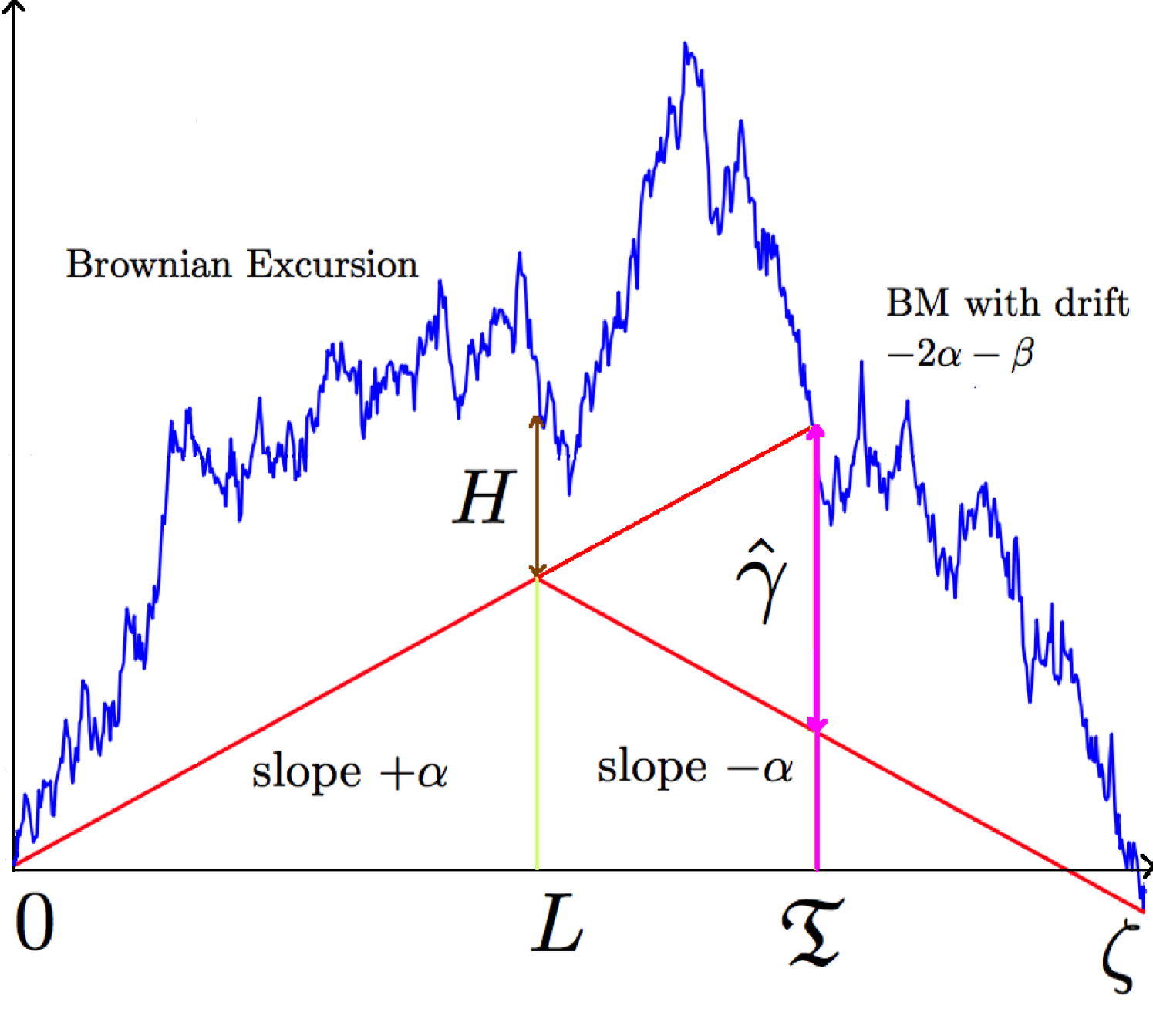
Now we have an explicit path decomposition of a generic excursion and we know the expression of the -Lipschitz minorant on the same interval in terms of the locations of the excursion at its end-points using Lemma 7.5. It is interesting to identify the distributions of the most important features such as:
-
•
the lifetime of the excursion;
-
•
the time at which the -Lipschitz minorant of the excursion attains its maximal value;
-
•
the final value of the excursion
— see Figure 5.1.
Proposition 5.8.
-
(i)
The joint Laplace transform of is
-
(ii)
The Laplace transform of the excursion length is
In particular, for the probability density of is
where .
-
(iii)
The Laplace transform of the time to the peak of the minorant during the excursion is
The corresponding density is
-
(iv)
The Laplace transform of the time after the peak of the minorant during the excursion is
The corresponding density is
-
(v)
The Laplace transform of , the final value of the excursion, is
We give the proof of Proposition 5.8 below after some preparatory results. We first recall a result about the distribution of the first hitting time of a Brownian motion with drift. [BS02, equations 2.0.1 & 2.0.2, page 295]
Lemma 5.9.
Let ( a Brownian motion with drift started at zero. Let and define . The density function of is
and its Laplace transform is
For the sake of completeness, we include the proof of the following simple lemma.
Lemma 5.10.
For ,
Proof.
Suppose without loss of generality that . We have
where in the third equality we used the substitution and in the fourth equality we used the fact that . ∎
We now give the proof of Proposition 5.8.
Proof.
We claim that
| (5.5) |
The stated equation for then follows by noting that
The Laplace transforms for the individual random variables follow by specialization and the claimed expressions for densities then follow from standard inversion formulas.
Rather than deriving (5.5) we will instead derive directly the Laplace transform of . This illustrates the method of proof with less notational overhead. We have
for
A little algebra shows that
Hence, using Lemma 5.10, we get that
After multiplying top and bottom by the conjugate this has following simple form
∎
Remark 5.11.
(i) Write for the difference between the Brownian motion and its minorant at time — see Figure 5.1. We can get an explicit description for the distribution of this random variable, though computing either its Laplace transform or density seems tedious to do. Indeed we know that for every , we have that , where for three independent standard Gaussian random variables. Hence,
where . Using the density in Theorem 5.7 and a change of variable gives that the joint density of at the point is
and independent of .
(ii) Set . From the time-reversal symmetry , we expect that
and this is indeed the case. This symmetry is somewhat surprising, as it is certainly not apparent from our path decomposition. Similarly, from the Brownian scaling , , we expect that
and this also holds.
(iii) It follows from the proposition that
Similarly,
and
Note that since almost surely, we expect by a renewal–reward argument.
(iv) The results of this section advance the study of the excursion straddling zero in the case of the Brownian motion with drift carried out in [AE14, Section 8]. Indeed, the previous study only determined the four-dimensional distribution , where and . Our approach here gives the distribution of the whole path of a generic excursion. Let us define
and
By Corollary 4.7, we have
Because we know the distribution of , the distribution of the straddling excursion can be recovered. In particular, the distribution of is just the size-biasing of the distribution of ; that is, for any nonnegative measurable function . For example, the joint Laplace transform of the analogues of for the straddling excursion is
Finally, if we denote by the Lévy measure of the subordinator associated with the regenerative set , then it has the density given by the following formula
(recall that is only defined up to a multiplicative constant).
6. Enlargement of the Brownian filtration
In this section, the Lévy process is the standard two-sided linear Brownian motion. Set
From [RY05, Chapter 3, Proposition 2.10] is then right-continuous and is a -two-sided linear standard Brownian motion. We denote the -Lipschitz minorant of and we let be defined, as above, by
By Lemma 7.3, the random time can be constructed as follows. Consider first the stopping time given by
Then
Thus, if we introduce the one-sided Brownian motion which is independent of , and we let be the time at which the process hits its ultimate infimum (this point is almost surely unique), then
As we have seen previously, the random time is not a stopping time. However, is an honest time in the sense of the following definition.
Definition 6.1.
Let be a random variable with values in , is said to be honest with respect to the filtration if, for every , there exists an -measurable random variable such that on the set we have .
Lemma 6.2.
The random time is an honest time. Moreover, if is a stopping time, then .
Proof.
We can write on the event as
The right-hand side is -measurable and hence is an honest time. Also, for any stopping time because whereas . ∎
We introduce now a larger filtration that is the smallest filtration containing that makes a stopping time.
Notation 6.3.
For , set
Remark 6.4.
Our goal now is to verify that every -semimartingale remains a -semimartingale, and to give a formula for the canonical semimartingale decomposition in the larger filtration.
Definition 6.5.
For any random time , we call the -supermartingale defined by
the Azéma supermartingale associated with . We choose versions of the conditional expectations so that this process is càdlàg.
We recall the following result from [Bar78, Theorem A].
Theorem 6.6.
Let be an honest time. A local martingale is a semimartingale in the larger filtration and decomposes as
where is a -local martingale.
It remains to find an explicit formula for . Define a decreasing sequence of stopping times that converges almost surely to by
Define the random times by
Note that almost surely because and with probability . Hence,
If we apply Lemma 8.1 for and we get
where . Now we use the following theorem from [Nik06, Theorem 8.22] .
Proposition 6.7.
Let be a continuous local martingale such that and . Let . Set
Then, the Azéma supermartingale associated with the honest time is given by
We apply Proposition 6.7 to our case for and the filtration .
By definition, we have , where . Set
The process is clearly a local martingale that verifies the conditions of the last proposition and we also have
Hence
Finally, we get the expression of the Azéma supermartingale associated with as
That is,
Thus, by sending , we get that
Now, using Theorem 6.6, every -local martingale is a -semimartingale and decomposes as follows
where denotes a -local martingale.
We develop further the expression of to get an explicit integral representation of its local martingale part.
Lemma 6.8.
Let be a standard Brownian motion and . Define the process by
Put . Then,
Proof.
Applying Itô’s formula on the semimartingale , where , gives
The last line follows from the fact that the measure is carried on the set . ∎
Put . We want to write the integral as a stochastic integral with respect to the original Brownian motion . For that we consider the time-change defined by . It is clear that this a family of stopping times such that the maps are almost surely increasing and continuous. Using [RY05, Chapter V, Proposition 1.5], we get that for every bounded -progressively measurable process we have
In our case this becomes
Hence,
Finally,
where
that is,
The process is decreasing and so the -local martingale part of is equal to
From the integral representation of martingales with respect to the Brownian filtration (see [RY05, Chapter 5, Theorem 3.4], every bounded -martingale can be written as
Such a process decomposes as a -semimartingale in the following way
where is a -local martingale.
7. General facts about the -Lipschitz minorant
Recall that a function admits an -Lipschitz minorant if and only if is bounded below on compact sets, , and . In this case,
| (7.1) |
The following result is obvious from (7.1).
Lemma 7.1.
Suppose that is a function with an -Lipschitz minorant. For , define by . Write and for the respective -Lipschitz minorants of and . Then .
The next result is a consequence of [AE14, Corollary 9.2] and Lemma 7.1, but we include a proof for the sake of completeness.
Lemma 7.2.
Consider a function for which the -Lipschitz minorant exists. Fix such that . Define by
Denote the -Lipschitz minorant of by . Then for all .
Proof.
From the expression of we have for every
Note that
and so for .
For the reverse inequality, it suffices to prove that
By definition, for all , and so, by the triangle inequality,
for every . ∎
The following result is [AE14, Lemma 9.4].
Lemma 7.3.
Let be a càdlàg function with -Lipschitz minorant . Set
and
Suppose that . Then, .
Let us also state here a simple expression of the time when the time zero is a contact point.
Lemma 7.4.
Let be a continuous function with -Lipschitz minorant , and suppose that we have , then defined in Lemma 7.3 takes the following form
Proof.
This is straightforward, as
because . ∎
The following lemma describes the shape of the -Lipschitz minorant between two consecutive points of the contact set. It is [AE14, Lemma 8.3].
Lemma 7.5.
Suppose that that is a càdlàg with -Lipschitz minorant . The set is closed. If t’<t” are such that , , and for all , then setting ,
8. Two random time lemmas
We detail in this section two lemmas that we used previously in Section 3 and Section 6. We consider here to be two-sided Lévy process with as its canonical right-continuous filtration; that is, , .
Lemma 8.1.
Let be a -stopping time that takes values in a countable subset of . Define the -fields , , and put . For every random variable measurable with respect to we have for every and that almost surely
Proof.
The first equality is trivial because the event is -measurable and hence -measurable. We therefore need only prove the second equality.
By a monotone class argument, it suffices to show that the second inequality holds for , where and are nonnegative Borel functions.
We have for any -measurable nonnegative random variable that
Using the independence and stationarity of the increments of the Lévy process gives
for . Thus,
Because the process is itself a Lévy process with respect to the filtration and it has the same distribution as , we have
Thus we finally get the desired equality
∎
Lemma 8.2.
Suppose that almost surely and that zero is regular for for the process . Let be a -stopping time. Put . Consider the random time . Then, setting , the -field is independent of the -field .
Proof.
We begin with an observation. Define the -fields , , and put . It follows from the part of the proof of Theorem 3.5 which comes before we employ the current lemma that is independent of
Returning to the statement of the lemma, and by noticing that , it suffices to prove for any bounded, nonnegative -measurable random variable , any bounded, nonnegative, continuous functions , and any previsible processes with respect to the filtration that
| (8.1) |
However, is itself a previsible process, so it suffices for (8.1) to prove for any bounded, nonnegative -measurable random variable , any bounded, nonnegative process that is previsible with respect to filtration , and any bounded, nonnegative, continuous functions that
| (8.2) |
A stochastic process viewed as a map from to is previsible with respect to the filtration if and only if it is measurable with respect to the -field generated by the maps , where ranges through the set of -valued -stopping times (see [RW87, Chapter IV, Corollary 6.9] for the analogous fact about previsible processes indexed by ). Also, note that the collection of the sets is a -system because the minimum of two stopping times is a stopping time. Hence, to establish (8.2), it suffices by a monotone class argument to show for any -valued -stopping time that
| (8.3) |
Because we have that , it further suffices to check (8.3) for an -valued -stopping time.
Consider (8.3) in the special case when and take values in the countable set . We then have
By applying Lemma 8.1 for , we have, for , that
Moreover, if we let to be an event in , then
because the process is clearly an -optional process (as it is the product of the left-continuous, right-limited -adapted process and the càdlàg -adapted process ). Hence
Substituting in this equality gives
We have thus proved (8.3) when and both take values in the set . Suppose now that is an arbitrary -valued stopping time but that still takes values in . For set when , . Thus is a decreasing sequence of -stopping times converging to . Taking (8.3) with replaced by and letting we get (8.3) for taking values in the set and general -valued .
We now to extend to the completely general case of (8.3). Put . Denote the corresponding random variables , , and by ,, and , respectively. Recalling that is an arbitrary bounded, nonnegative random variable measurable with respect to , it suffices by a monotone class argument it suffices to show (8.3) in the special case where
for , , bounded, nonnegative, continuous functions and .
For set when , . Thus is a decreasing sequence of -stopping times converging to . Note that
Thus, if , then by the right-continuity of the sample paths of . On the other hand, if , then, for large enough, we have that . Hence, by applying the special case of (8.3) for the stopping times taking discrete values, and using the fact that has càdlàg paths we get
which finishes our proof. ∎
References
- [AE14] Joshua Abramson and Steven N. Evans, Lipschitz minorants of Brownian motion and Lévy processes., Probab. Theory Relat. Fields 158 (2014), no. 3-4, 809–857 (English).
- [Bar78] M. T. Barlow, Study of a filtration expanded to include an honest time, Z. Wahrsch. Verw. Gebiete 44 (1978), no. 4, 307–323. MR 509204
- [BB03] François Baccelli and Pierre Brémaud, Elements of queueing theory, second ed., Applications of Mathematics (New York), vol. 26, Springer-Verlag, Berlin, 2003, Palm martingale calculus and stochastic recurrences, Stochastic Modelling and Applied Probability. MR 1957884
- [Ber96] Jean Bertoin, Lévy processes, Cambridge Tracts in Mathematics, vol. 121, Cambridge University Press, Cambridge, 1996. MR 1406564 (98e:60117)
- [BS02] Andrei N. Borodin and Paavo Salminen, Handbook of Brownian motion—facts and formulae, second ed., Probability and its Applications, Birkhäuser Verlag, Basel, 2002. MR 1912205 (2003g:60001)
- [FT88] P. J. Fitzsimmons and Michael Taksar, Stationary regenerative sets and subordinators, Ann. Probab. 16 (1988), no. 3, 1299–1305. MR 942770 (89m:60176)
- [GP80] Priscilla Greenwood and Jim Pitman, Construction of local time and Poisson point processes from nested arrays., J. Lond. Math. Soc., II. Ser. 22 (1980), 183–192 (English).
- [GS74] R. K. Getoor and M. J. Sharpe, Last exit decompositions and distributions, Indiana Univ. Math. J. 23 (1973/74), 377–404. MR 0334335 (48 #12654)
- [Jeu79] Thierry Jeulin, Grossissement d’une filtration et applications, Séminaire de probabilités de Strasbourg 13 (1979), 574–609 (fr). MR 544826
- [Kal02] Olav Kallenberg, Foundations of modern probability, second ed., Probability and its Applications (New York), Springer-Verlag, New York, 2002. MR 1876169 (2002m:60002)
- [Mil77] P. W. Millar, Zero-one laws and the minimum of a Markov process, Trans. Amer. Math. Soc. 226 (1977), 365–391. MR 0433606 (55 #6579)
- [Mil78] by same author, A path decomposition for Markov processes, Ann. Probability 6 (1978), no. 2, 345–348. MR 0461678 (57 #1663)
- [Nev77] J. Neveu, Processus ponctuels, 249–445. Lecture Notes in Math., Vol. 598. MR 0474493
- [Nik06] Ashkan Nikeghbali, An essay on the general theory of stochastic processes, Probab. Surveys 3 (2006), 345–412.
- [Pit83] J. W. Pitman, Remarks on the convex minorant of Brownian motion, Seminar on stochastic processes, 1982 (Evanston, Ill., 1982), Progr. Probab. Statist., vol. 5, Birkhäuser Boston, Boston, MA, 1983, pp. 219–227. MR 733673 (85f:60119)
- [Pit87] Jim Pitman, Stationary excursions, Séminaire de Probabilités, XXI, Lecture Notes in Math., vol. 1247, Springer, Berlin, 1987, pp. 289–302. MR 941992
- [PS72] A. O. Pittenger and C. T. Shih, Coterminal families and the strong Markov property, Bull. Amer. Math. Soc. 78 (1972), 439–443. MR 0297019 (45 #6077)
- [RP81] L. C. G. Rogers and J. W. Pitman, Markov functions., Ann. Probab. 9 (1981), 573–582 (English).
- [RW87] L. C. G. Rogers and David Williams, Diffusions, Markov processes, and martingales. Vol. 2, Wiley Series in Probability and Mathematical Statistics: Probability and Mathematical Statistics, John Wiley & Sons Inc., New York, 1987, Itô calculus. MR 921238 (89k:60117)
- [RY05] Daniel Revuz and Marc Yor, Continuous martingales and Brownian motion. 3rd ed., 3rd. corrected printing., 3rd ed., 3rd. corrected printing ed., vol. 293, Berlin: Springer, 2005 (English).
- [Sat99] Ken-iti Sato, Lévy processes and infinitely divisible distributions, Cambridge Studies in Advanced Mathematics, vol. 68, Cambridge University Press, Cambridge, 1999, Translated from the 1990 Japanese original, Revised by the author. MR 1739520 (2003b:60064)
- [SH04] F.W. Steutel and K. Harn, van, Infinite divisibility of probability distributions on the real line, Pure and applied mathematics : a series of monographs and textbooks, Marcel Dekker Inc., United States, 2004 (English).
- [Tho00] Hermann Thorisson, Coupling, stationarity, and regeneration., New York, NY: Springer, 2000 (English).