Existence of quasi-static crack evolution for atomistic systems
Abstract.
We consider atomistic systems consisting of interacting particles arranged in atomic lattices whose quasi-static evolution is driven by time-dependent boundary conditions. The interaction of the particles is modeled by classical interaction potentials where we implement a suitable irreversibility condition modeling the breaking of atomic bonding. This leads to a delay differential equation depending on the complete history of the deformation at previous times. We prove existence of solutions and provide numerical tests for the prediction of quasi-static crack growth in particle systems.
Key words and phrases:
Atomistic systems, delay differential equations, minimizing movements, quasi-static crack growth, irreversibility condition1. Introduction
The theory of brittle fracture is based on the fundamental idea that the formation of cracks may be seen as the result of the competition between the elastic bulk energy of the body and the work needed to produce a new crack. Despite its long history in mechanics dating back to [29], a rigorous mathematical formulation of the problem is much more recent: in the variational model of quasi-static crack growth proposed in [22], displacements and crack paths are determined from an energy minimization principle, reflecting suitably the three foundational ingredients of Griffith’s theory: (1) a surface energy associated to discontinuities of the deformation, (2) a propagation criterion for those surfaces, and (3) an irreversibility condition for the fracture process.
The mathematical well-posedness of the variational model [22] has been the subject of several contributions over the last two decades, see e.g. [16, 17, 21, 27]. The proof of continuous-time evolutions is based on approximation by time-discretized versions resulting from a sequence of minimization problems of so-called Griffith functionals, being variants of the Mumford & Shah functional [31]. Functionals of this type comprising elastic bulk contributions for the sound regions of the body and surface terms along the crack have been studied extensively in the last years in the natural weak framework of special functions of bounded variation. We refer to [6] for a thorough overview of the variational approach to fracture. In particular, it has been shown that such continuum models can be identified as effective limits derived from atomistic systems as the interatomic distance tends to zero [12, 14, 24]. Asymptotic analysis of this kind is notoriously difficult, and is not based on simply taking pointwise limits but rather on a variational convergence, called -convergence [15], which in this setting ensures convergence of minimizers of the atomistic system to the ones of the continuum problem.
Although studies on atomistic-to-continuum passages are flourishing, most results are static and the evolutionary nature of processes is mostly neglected. Our goal is to advance this understanding by establishing a rigorous connection between atomistic and continuum models in brittle fracture for the prediction of quasi-static crack growth. In this contribution, we perform the first step in this direction by setting up a suitable quasi-static model on the atomistic level respecting the irreversibility condition of Griffith’s theory. The passage to continuum models of quasi-static crack growth will be discussed in a forthcoming work [26].
We consider atomistic systems consisting of interacting particles arranged in an atomic lattice occupying a bounded region representing the reference domain of a material. The interaction of the atoms is modeled by classical potentials in the frame of Molecular Mechanics, e.g. by Lennard-Jones potentials. Based on an energy minimization principle, the deformation of the particles is driven by time-dependent boundary conditions. This leads to an evolution of gradient-flow type. Whereas the study of interacting particles motion is classical, the novelty of our contribution lies in implementing an irreversibility condition along the evolution. As long as the length of interactions does not exceed a certain threshold, interactions are considered to be ‘elastic’ and can recover completely after removal of loading. Otherwise, interactions are supposed to be ‘damaged’, and the system is affected at the present and all future times. Here, we suitably adapt the maximal opening memory variable used in continuum models for cohesive crack evolutions [18, 28] to the atomistic setting.
This results in a delay differential equation taking the complete history of the deformation into account. Our approach is based on the assumption that the boundary loading varies slowly in time compared to the elastic wave speed of the material. Therefore, inertial effects are neglected, and the delay differential equation is a first order equation in time. Our main result consists in proving existence of solutions, see Theorem 2.2, where the strategy relies on a time-incremental scheme, the so-called minimizing movement scheme for gradient flows [4, 19, 32]. Similarly to the continuum model [21], due to the presence of an irreversibility condition and the memory effect, the main difficulty lies in the passage to the limit as the time-discretization step tends to zero. In particular, we use an evolutionary model of rate type in order to obtain uniform convergence in time as . This allows to pass to the limit in the memory variable, see Remark 4.3 for some details.
Let us highlight that our approach is rather simplistic and does not reflect the physical reality of fracture in brittle substances in its whole complexity. On the one hand, our modeling of elastic and damaged interactions is not justified by formation and dissociation of chemical bonding but inspired by a continuum mechanics perspective on brittle fracture. In this sense, we believe that our model may be relevant as a discretization of quasi-static crack evolution from continuum theory. On the other hand, physically relevant interatomic potentials describing the behavior of brittle materials need to encompass multi-body contributions, at least three-body potentials [11, 35, 36]. Following the approach of several studies on variational atomistic fracture [1, 7, 8, 10, 23], we focus here on configurational energies consisting purely of pair interactions. Nevertheless, we present a possible extension of our model to three-body potentials in Subsection 2.4.
Our analysis is at the basis of a forthcoming work [26] where we study the evolution of the model in the passage to continuum problems, i.e., when the interatomic distance tends to zero. Indeed, in the static case, -limits of suitable atomistic systems can be identified as free discontinuity functionals of Griffith-type [14, 24] featuring a linearly elastic bulk energy and surface contributions proportional to the length of the crack. For these continuum models, existence results for quasi-static crack evolutions have been derived in [21, 27]. We will identify evolutions of this form as limits of the solutions to the atomistic delay differential equations in the atomistic-to-continuum limit.
The paper is organized as follows. In Section 2 we introduce the model and present the main results. Section 3 is devoted to some explicit examples of possible atomistic systems, and provides several numerical experiments of our model in one and two dimensions. Eventually, Section 4 contains the proofs of our results. We close the introduction with some notation. In the following, we denote by the standard Euclidean norm in for . For the scalar product of two vectors , we write . We let for . As usual, generic constants in proofs are denoted by and may change from line to line.
2. The model and main results
2.1. Deformations and interaction energy
We describe the atomistic deformation of a material occupying an open, bounded set in dimension . By we denote an arbitrary but fixed lattice, and let be the positions of the atoms (or particles) in the specimen in the reference configuration. The deformation of the particles is described through a map , where for each the vector indicates the position of in the deformed configuration. (The typical choice is .)
We model the interaction of the atoms by classical potentials in the frame of Molecular Mechanics [2, 30]: given a deformation , we assign a phenomenological energy to the deformation by
| (2.1) |
where denotes a smooth two-body interaction potential, with . The factor accounts for the fact that every contribution is counted twice in the sum. It is also possible that the sum ranges only over a subset of all pairs by simply setting for certain interactions. Whenever , the potential is supposed to be repulsive for small distances and attractive for long distances, a classical choice being a potential of Lennard-Jones-type. More specifically, we assume that satisfies
-
(i)
;
-
(ii)
is minimal if and only if with ;
-
(iii)
is decreasing for and increasing for ;
-
(iv)
.
The repulsion effect (i) describes the Pauli repulsion at short distances of the interacting particles due to overlapping electron orbitals, and (ii)-(iv) correspond to attraction at long ranged interactions vanishing at infinity. Some toy examples of lattices and possible configurational energies are given below in Section 3. Let us mention that we restrict our model to pair interactions equilibrated in the reference configuration (see Assumption (ii)) for mere simplicity. The model could be generalized to pre-stressed interactions, and multi-body, non-local, and multiscale energies could be considered, see e.g. [12] for a very general framework. We include, however, non-homogeneous interactions as all potentials can be different. A possible extension featuring three-body potentials is addressed in Subsection 2.4 below.
By we denote the minimal interatomic distance. A huge body of literature deals with effective descriptions of atomistic energies of the form (2.1) when the interatomic distance tends to . This passage from atomistic to continuum models is nontrivial even for simple energies and might lead to very different asymptotic behavior, see [5] for taking pointwise limits and [9] for an overview of a variational perspective. For interaction densities of the above form, it has been shown in [14, 24] that effective continuum energies lead to so-called Griffith energy functionals featuring both bulk and surface terms. In the present contribution, the number of atoms and are fixed. The study of an evolutionary model as is deferred to a forthcoming paper [26].
Following the discussion in [33, 24], we impose Dirichlet boundary condition on a part of the boundary. More precisely, consider a neighborhood of such that . For a function , we define the admissible deformations by
Instead of (or additional to) Dirichlet boundary conditions, one could also consider body or boundary forces. However, as traction tests with body forces are ill-posed for Griffith functionals in a continuum variational formulation, we prefer to focus on boundary value problems also on the atomistic level. For a thorough discussion on the comparison of soft and hard devices in the context of the variational formulation of Griffith’s fracture, we refer the reader to [6, Section 3].
2.2. Evolutionary model: Irreversibility condition and memory variable
Based on the energy (2.1), we will now introduce an evolutionary model on a process time interval , where the evolution will be driven by time dependent boundary conditions . The key feature in the modeling is to implement an irreversibility condition along the fracture process for each pair interaction of , once the length of the interaction exceeds the elastic regime. As long as does not surpass a threshold satisfying , the pair interaction can recover completely after removal of loading. By contrast, if exceeds at some earlier time, the interaction is supposed to be ‘damaged’, and the system should be affected at the present time, i.e., the complete history of the deformation undergone by the atomistic system should be reflected at present time. This corresponds to a model of cohesive type energy á la Barenblatt [13].
To describe this, we fix , a deformation at time , and suppose that a finite or infinite family of deformations at previous times is given. The interaction of at time is considered to be elastic if for all . Otherwise, we adopt as memory variable the maximal opening as implemented, e.g. in the continuum models [18, 28], see also [6, Section 5.2]. Writing
| (2.2) |
for the memory variable, the energy contribution with memory reads as
| (2.3) |
Other choices, such as that of a cumulative increment, could also be made, but are not discussed in this paper. Note that by implementing the memory variable, the repulsion effect for small distances (Assumption (i)) is lost and (2.3) does not describe correctly the Pauli repulsion at short distances of the interacting particles. Therefore, for the energy contribution of a damaged interaction we rather use
Clearly, by Assumption (iii) this is equal to
| (2.4) |
This notion is rather simplistic and one drawback lies in the sharp transition between elastic and inelastic behavior. To remedy this, we introduce a second threshold and assume that in the transition zone the interaction can partially recover, i.e., the energy contribution still partly depends on the current deformation. Let be continuous and increasing with for and for . Define the energy contribution as
| (2.5) | ||||
Note that formally this would correspond to (2.4) for the (not admissible) choice for and for . In particular, (2.5) implies
We adopt the choice (2.5) for a continuous function interpolating between and also for technical reasons, see the discussion in Remark 4.3. Summarizing, given the history , the energy of an admissible configuration is given by
| (2.6) |
2.3. Quasi-static evolution of atomistic systems with damageable interactions
We now present the main result of the paper on a quasi-static evolution of atomistic systems with the irreversibility condition introduced above. We introduce some further notation. Let be the cardinality of and let be the cardinality of , respectively. For convenience, from now on we will denote as a single vector via
where is a fixed numbering of with . In this sense, in (2.6) is a function defined on with variables . We also regard boundary conditions as vectors for each by setting for all .
As it is customary in both existence proofs and in numerical approximation schemes, we start with a time-discretization of the problem. Fix a discrete time step size , which for simplicity satisfies . We write for , and we also define . Suppose that an initial configuration is given. Fix a time and suppose that the deformations at the previous times , , have already been found. Then, the deformation at time , denoted by , is given as the minimizer of
| (2.7) |
Here, denotes the Euclidean norm in , where is a dissipation coefficient. We remark that (2.7) corresponds to the minimizing movement scheme for gradient flows of the energy with respect to the -norm. At the end of the section, see (2.11), we present a variant of (2.7) which corresponds to a model in the Kelvin-Voigt’s rheology. Note that an essential part of our problem is the fact that the energy depends on the complete history, i.e., on the previous deformations , which is usually not present in incremental schemes of the form (2.7). Let us mention that this relates to a discrete-time formulation where, in contrast to common variational approaches to fracture in the realm of rate-independent systems, in each step we do not consider absolute minimizers of the energy, but determine local minimizers by penalizing the -distance between the approximate solutions at two consecutive times. This approach itself is not new and has been adopted, e.g. in [17].
Note that the existence of a minimizer is readily guaranteed since the problem is finite dimensional, the potential is continuous, and the energy is coercive. Moreover, one can also check that for sufficiently small the problem is strictly convex, and therefore the minimizer is unique.
We now introduce piecewise constant and piecewise affine interpolations by for and for , respectively, where . Our goal is to pass to the limit , and to prove that converges uniformly to a limit evolution , which satisfies a delay differential equation taking the irreversibility of the fracture process into account. We start with the compactness result.
Theorem 2.1 (Compactness).
Assume that . Suppose that an initial datum is given, and let and be constructed as above. Then, there exists with for all such that and converge uniformly to on , as well as weakly in .
We are now ready to present the main result of the paper.
Theorem 2.2 (Quasi-static evolution for damageable pair interactions).
Given an initial value , denote by the function identified in Theorem 2.1. Then, satisfies the delay differential equation
| (2.8) |
Here, is taken with respect to the variables , i.e., both sides in (2.8) are vectors in . More explicitly, (2.8) can be written as
Although the potentials are smooth, is not necessarily differentiable due to the presence of the memory variable. Therefore, strictly speaking, has to be interpreted as the element of the subdifferential of (in the sense of -convex functions) with minimal norm, denoted by . We refer to (4.16)–(4.17) for details.
Let us highlight that the resulting equation is not an ordinary differential equation of gradient flow type but a delay differential equation as the energy at time depends on the complete history .
2.4. Variants and possible extensions
We close this section by discussing alternative modeling assumptions and possible extensions. Let us start by presenting a variant of the model where the -dissipation is replaced by a dissipation depending on a (discrete) strain rate. This corresponds to a model in the Kelvin-Voigt’s rheology. For simplicity, we restrict our modeling here to the one-dimensional case () as proofs are more involved in higher dimensions. Specifically, we denote the reference configuration by with for , and denote deformations by . Let , where for convenience we use a different labeling of compared to Subsection 2.3. We introduce the discrete gradient by
| (2.9) |
We also introduce the vector defined by
| (2.10) |
We replace the time-incremental scheme described in (2.7) by
| (2.11) |
In the limit of vanishing time steps , this leads to the delay differential equation
| (2.12) |
where is explained in (4.16)–(4.17) and is taken with respect to . The proof is similar to the one of Theorem 2.2 and the necessary adaptions are given in Remark 4.4. Let us mention that a more realistic modeling assumption would be that is different for each contribution and depends on the memory variable , with decreasing in .
The model developed so far was restricted to pair interactions for the sake of simplicity. However, for a realistic description of brittle materials also multi-body interactions should be taken into account. Here, we present one possible simple extension incorporating three-body interactions. Let be three distinct neighboring atoms in the reference configuration with and . Consider the angle between the two edges and under the deformation , given by
Let be a continuous three-body interaction potential, see [11, 35, 36] for possible choices. We then assume that the three-body energy contribution of has the form
This reflects the assumption that the three-body-interaction is only active as long as the two interactions and are not ’damaged’. The total energy in (2.6) then changes to
| (2.13) |
Note that Theorem 2.2 stated above still holds for this extended model, as we briefly indicate after the proof of Theorem 2.2, see Remark 4.5.
3. Examples and numerical experiments
The proposed model for discrete crack evolution captures a variety of possible atomic interactions. In preparation for our numerical experiments, we discuss here simple models in 1D and 2D.
The easiest case consists in a one-dimensional set-up described at the end of Subsection 2.3 with nearest neighbor interactions. If it holds , and for the interaction takes the form
| (3.1) |
We also choose some parameters for the memory variable independently of .
In two dimensions, an important mathematical model is given by a triangular lattice and nearest neighbor interactions of the form (3.1). This model was considered in [24]. Here, the deformations are assumed to locally preserve their orientation, i.e., affine interpolation should have nonnegative determinant on each triangle of the lattice , cf. [33]. Additionally, one could also add next-to-nearest neighbors to the energy, i.e., the interaction of points , of the lattice opposite to the same edge (with distance ). In this case, we add
| (3.2) |
to the energy for each such pair, where and is given by (3.1).
We now describe numerical experiments for the 1D and the 2D case. In dimension one, we consider a chain of equally spaced atoms with interatomic distance . To ease numerical computations, we only consider interaction energies (2.6) of nearest-neighbor type as given in (3.1). We set , and for simplicity . As dissipation, we consider both cases mentioned above, i.e., the -distance and the Kelvin-Voigt-dissipation. We set and . The numerical computation of each step of the minimizing movements schemes in (2.7) and (2.11) is performed via an interior point optimizer [34] accessed through the JuMP modeling language [20].
In Figure 1, one can see 13 steps of both schemes. The evolution starts with the chain of atoms with distance to each other. The boundary condition fixes one of the endpoints while driving the other endpoint in sinusoidal motion stretching and compressing the chain in the process. In both cases, the chain first extends elastically and at some point one of the bonds between neighboring atoms breaks. While in the case of Kelvin-Voigt, by symmetry, any of the bonds is equally likely to break (in the specific case above it is the -th bond), the -dissipation always favors the very last bond since already for small loading this bond is stretched the most. After compression, in the second turn of extension, no elastic stretching can be observed since one bond is already broken.
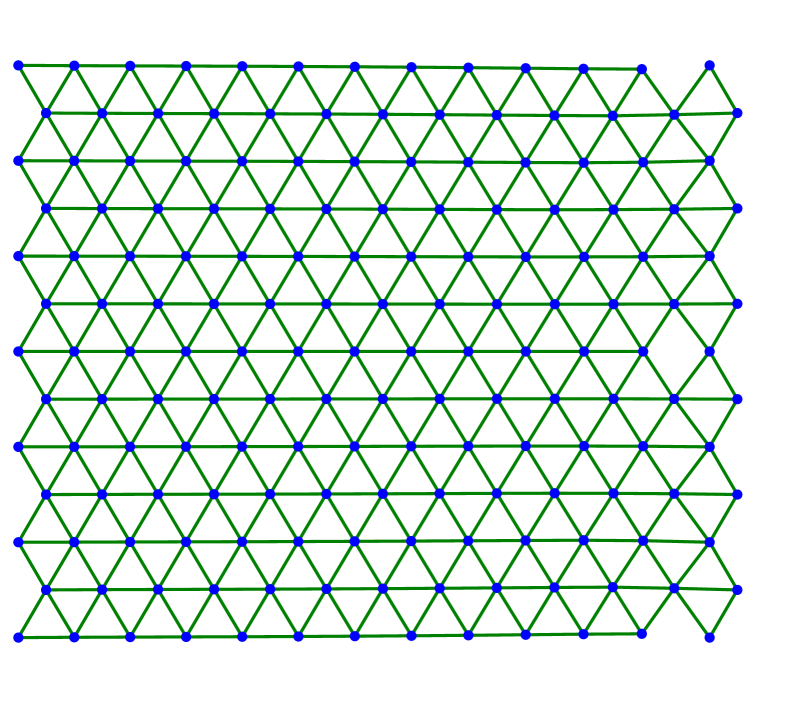
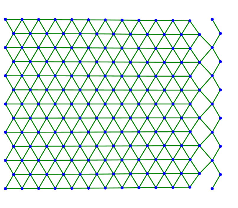
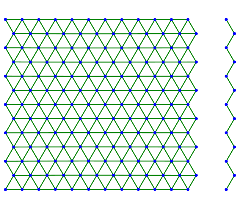
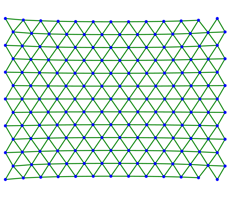
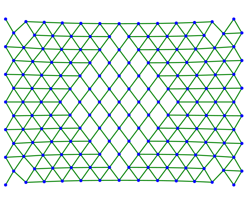
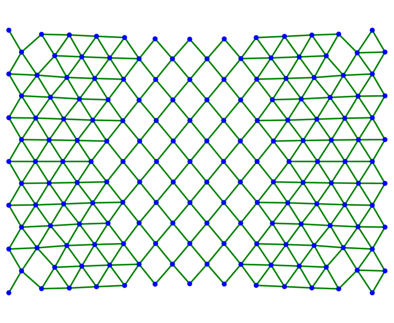
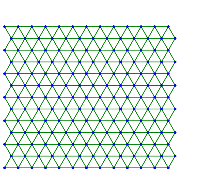
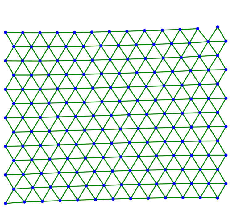
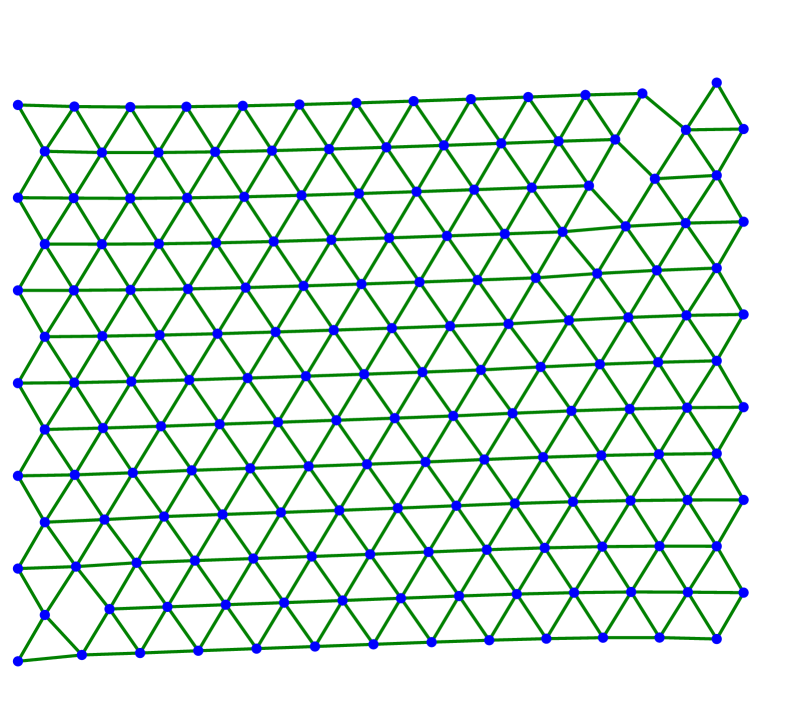
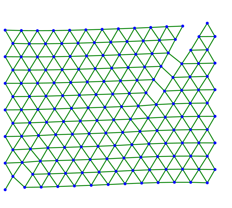
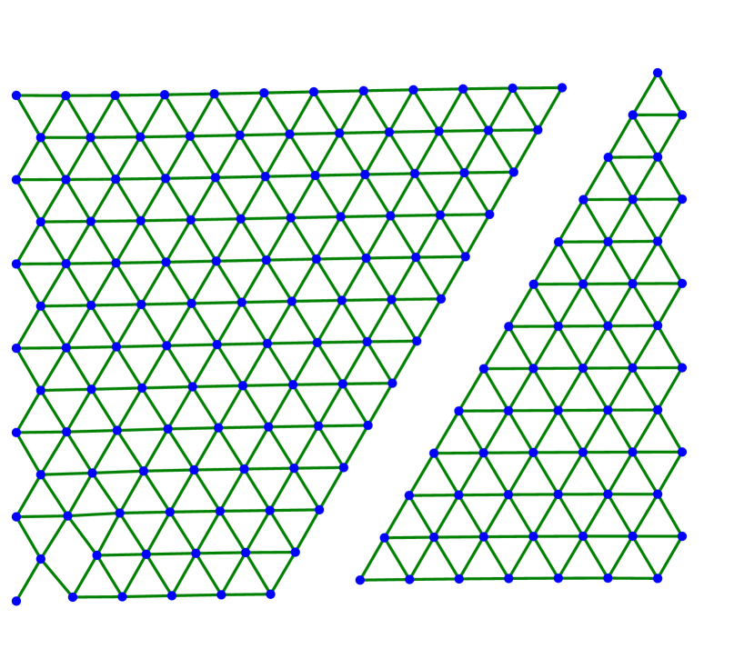
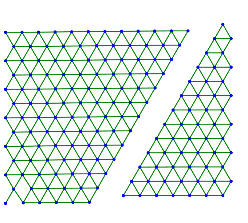
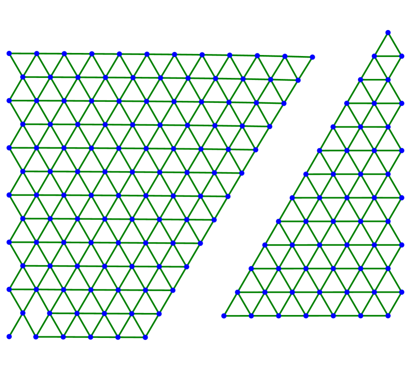
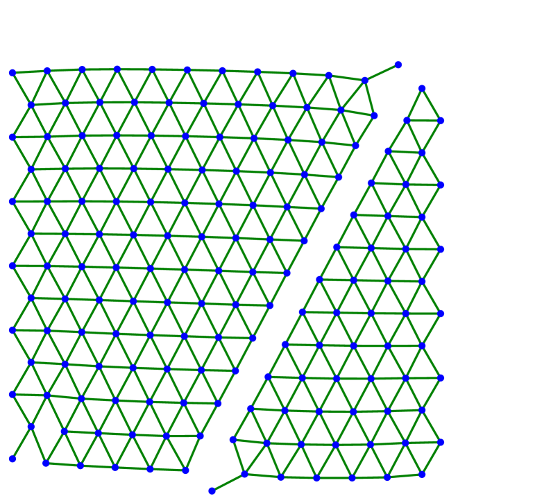
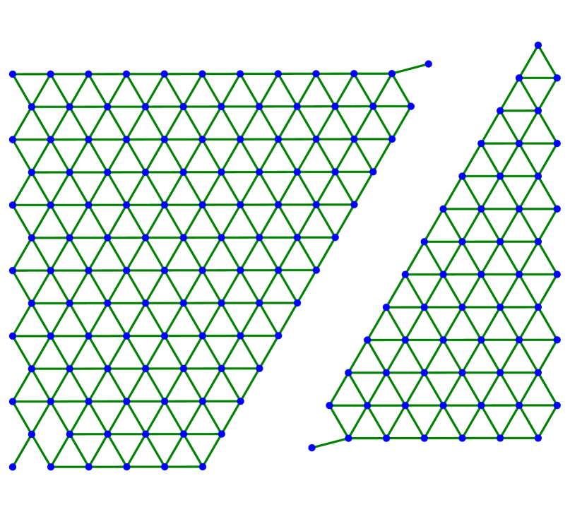
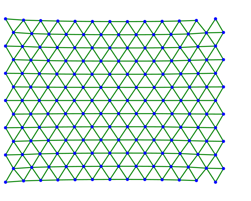
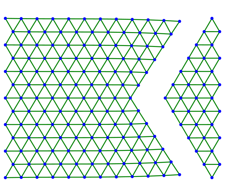
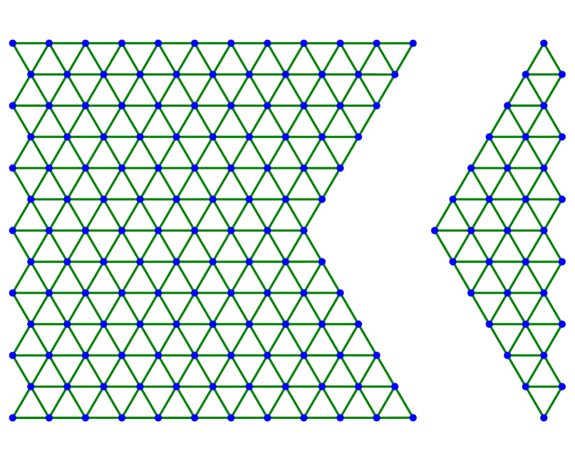
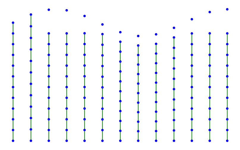
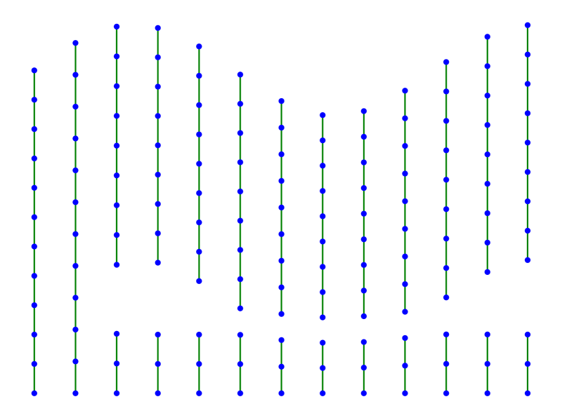
We continue by showing several examples in two dimensions. In all cases, we consider the triangular lattice with nearest neighbors and next-to-nearest neighbors as described in (3.1)–(3.2) with . The evolution starts with a finite amount of atoms arranged in a lattice of equilateral triangles. The left-most atoms are fixed along the evolution while the right-most atoms are stretched horizontally or with respect to some angle.
Figure 2 shows the case of a large value for horizontal stretching. Figures 2(a)–2(c) depict three steps of the scheme with -dissipation, where the right-most layer of atoms detaches from the material. Figures 2(d)–LABEL:sub@fig:square_kv_3 shows steps arising from a Kelvin-Voigt-type dissipation. In this case, the material does not develop a sharp crack interface. Instead, starting from the center more and more horizontal bonds are broken. This suggests that should be chosen much smaller.
Figure 3 shows several steps of the respective minimizing movement scheme with -dissipation and small dissipation coefficient . In contrast to Figure 2, we use sinusoidal boundary conditions that move the right-most points of the lattice upwards in direction . As predicted in [23, 25] for the static case, the lattice breaks apart along a crystallographic line, see Figures 3(f) and 3(g). The two components are stopped from colliding into each other in the subsequent compression phase (see Figure 3(h)). After stretching once more, the components separate from each other reaching the final state in Figure 3(i). Although not shown here, the evolution arising from a dissipation of Kelvin-Voigt type does essentially not differ from the one shown in Figure 3. Furthermore, Figure 4 shows an experiment with boundary conditions in horizontal direction. Due to the symmetry of the lattice, the crack line can be kinked, in accordance to [23, 25].
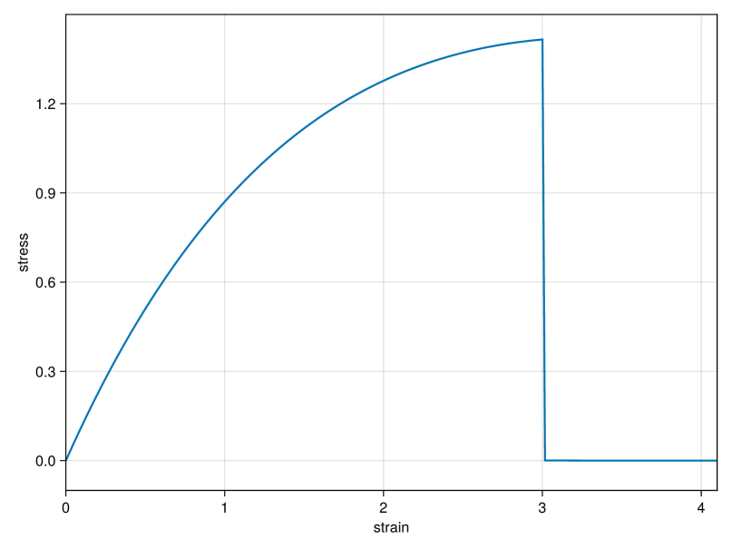
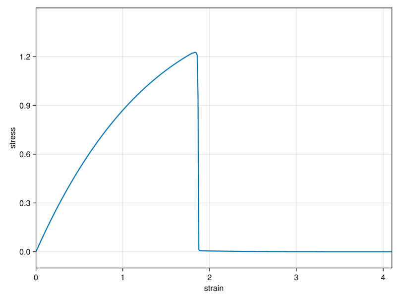
Eventually, in Figure 5 we plot the stress-strain curve that corresponds to the stretching phase in a tension-compression experiment similar to the one shown in Figure 3. More precisely, we computed the total stress , suitably normalized by the number of boundary interactions. As the material is stretched, the stress increases almost linearly until the formation of a crack where the stress drops to zero. The flattening of the curve for higher strains is due to the nonlinearity of the interaction potentials. In case of a smaller crack-threshold , the material breaks already at a smaller loading. Accordingly, the flattening of the curve is less pronounced and the maximal value of the stress, which corresponds to the transition from the elastic to the fracture phase, is smaller.
4. Proofs
4.1. Incremental minimization scheme
In this subsection, we analyze the scheme (2.7) for a given family of deformations . For convenience, we denote the memory variable simply by . In a similar fashion, we express the energy for fixed , by
| (4.1) |
and for the sum over all contributions we write
| (4.2) |
Furthermore, in this subsection we drop the superscript , i.e., we write and in place of and , respectively. By convention, in proofs we often drop the index for , , , , , if no confusion arises.
We begin by proving a lemma that follows from the very definition of the potential in (2.5) and the incremental minimization scheme described in (2.7).
Lemma 4.1.
Given a time step and deformations at previous time steps, let be defined as in (2.7). Then,
Proof.
It suffices to show that for all , . For simplicity, we drop the superscript in the proof. Recall that by definition (2.5) we have
| (4.3) |
where for and for . Note that by the definition of the memory variable in (2.2) we obtain
Case 1: We first consider pairs , , that fulfill . Then trivially holds.
Case 2: Let , , be such that . Then, we have
and since is increasing on by Assumption (iii) and we get
Hence, by (4.3) we obtain
which proves the assertion. ∎
As a next step, we prove an estimate that will enable us to control the time derivative of the deformation. As a preparation, consider for every . Then, using , the fundamental theorem of calculus, and Jensen’s inequality it follows that
| (4.4) |
and with Hölder’s inequality
| (4.5) |
We thus have the estimates
| (4.6) |
for a constant independent of .
Lemma 4.2.
There exists such that for each it holds that
| (4.7) |
Proof.
We prove the statement by induction. The case is trivial. Suppose that the estimate holds for . In particular, by (4.6) we get
| (4.8) |
for some depending on and but independent of . By choosing as a test function in the minimization problem (2.7) we get
| (4.9) |
We aim at estimating . As before, this can be reduced to considering each , . First, by Assumption (i) and (4.8) we get
| (4.10) |
for a constant depending on , , and , but independent of . By the regularity of and Assumption (iv) we find that is Lipschitz continuous on . Therefore, also is Lipschitz continuous on . We denote the Lipschitz constant by which is independent of .
We again drop subscripts and write , , , and for convenience. Note that for with and we have . Let and . Observe that by (4.10), and that for small enough since (4.6) implies
Then, we get
| (4.11) |
As for , we can also infer that
| (4.12) | ||||
Putting (4.1) and (4.12) together we derive for the energy contribution (see definition (4.3)) the estimate
| (4.13) |
From this estimate, summing over all pairs , we conclude
where is the maximum of the involved Lipschitz constants. Eventually, we get by Hölder’s inequality
| (4.14) |
Note that can be chosen independently of as the constants in (4.10) are independent of . Putting (4.9) and (4.14) together and rearranging terms yields
for some large enough. By Lemma 4.1 this becomes
This inequality added to (4.7) for gives the desired estimate (4.7) for . ∎
4.2. Compactness
In this subsection, we prove Theorem 2.1. For this reason, we again include the time step in our notation. After the preparation in Lemma 4.2 the proof is standard. We perform it here, however, for convenience of the reader.
Proof of Theorem 2.1.
The right-hand side of (4.7) for can be expressed in terms of as in (4.4)–(4.5). Thus, from (4.7) we obtain
for some , where in the last step we used the regularity of and the fact that is bounded from below. Considering the interpolation as introduced before Theorem 2.1, we derive
Therefore, is uniformly bounded in . By weak compactness we have, up to a subsequence,
In particular, is Hölder-continuous by the well-known inclusion and the convergence is uniform. In fact, by the fundamental theorem of calculus we get
and using Hölder’s inequality we deduce
By Arzelà-Ascoli, converges uniformly to the limit function . For and we define the piecewise affine interpolation . Then, by the fundamental theorem of calculus and Hölder’s inequality, for any it follows
where is the smallest natural number such that . This shows in . Note also that we have in for all since by construction on for all . This yields for all . It remains to observe that also the piecewise constant interpolation converges uniformly to . Indeed, we know that for every we have for a certain with . In particular, we get
This shows that also converges uniformly to (along the same subsequence). ∎
4.3. The limiting delay differential equation
Next, we consider the limiting evolution identified in Theorem 2.1, and give the proof of Theorem 2.2. We first introduce some additional notation. Recalling (4.1)–(4.2) we let
and for . Although the potentials are smooth, the function is possibly not differentiable if . Therefore, we need to introduce the concept of subdifferential for -convex functions, see e.g. [32]. As before, for convenience we drop in the notation. Recall that
for , see (4.3). In fact, by Assumption (iv) one observes that is -convex for some , i.e., is convex. In this case, the subdifferential is defined as
| (4.15) |
where and denote the vectors of images of under and , respectively. By the theory of subdifferentials we compute that
where whose entries are given by if , if , and if . Here, we use the notation . Note that for , the function is differentiable and therefore the subdifferential only consists of one element, whereas in the case it is given by an interval. If is not single valued, we denote by the element of minimal norm. In our case, this is
| (4.16) |
For the entire energy, this reads as
| (4.17) |
for , where as before denotes the element of minimal norm. After these preparations, we proceed with the proof of Theorem 2.2.
Proof of Theorem 2.2.
Since by construction , for times we obtain
| (4.18) |
where is again taken with respect to the variables , cf. (4.15). We aim to pass to the limit in this equation. The term on the left-hand side converges weakly to by Theorem 2.1. We thus consider the limit of the right-hand side.
Because of the uniform convergence , we particularly know that for an arbitrary pair of lattice points we have
With the continuity of , we thus obtain
| (4.19) |
Due to the fact that the convergence is uniform in time, we also get the continuity of with respect to , i.e., we get
| (4.20) |
as for each pair and all . With the definition in (2.2), this means
| (4.21) |
The convergences (4.19)–(4.20) and the continuity of allow us to go to the limit in , i.e.,
| (4.22) |
for all and all , where
depending on whether is bigger, smaller, or equal to . Summing over all pairs and recalling the definition of the energy in (2.6) we conclude
Now, passing to the limit in (4.18) we conclude
for almost every . Recalling the argumentation in [32, Proposition 2.2] we deduce that
for almost every . This concludes the proof. ∎
Remark 4.3 (Role of and viscosity ).
The delicate part in the above proof is the limiting passage in . In particular, the continuity of is essential in (4.22): if was not continuous instead, as in the possible modeling assumption for and for discussed in Subsection 2.2, it would not be clear how to obtain convergence as . We also mention that we consider a model of rate type with viscosity in order to control and thus to obtain uniform convergence. This is crucial in order to obtain continuity of the memory variable, see (4.21). For a model in the realm of rate-independent processes, uniform convergence cannot be guaranteed, and thus we possibly do not have continuity in (4.21).
Remark 4.4 (Proof of existence for (2.12)).
We briefly indicate the necessary adaptations in the proof in order to derive existence of solutions to (2.12). First, by an argument analogous to the one in Lemma 4.2 one can show that
| (4.23) |
By the triangle inequality we find for each that
By a discrete Hölder’s inequality we then find
Summation over all atoms and using for all time steps yields
where the last step follows from the definition in (2.9). This along with (4.23) as well as (4.6) shows
and at this point the compactness proof in Theorem 2.1 can be repeated. Concerning the passage , we only need to replace the inclusion (4.18) by
where is defined as in (2.10), and then we can pass to the limit on both sides as before.
Remark 4.5 (Extended model (2.13)).
5. Conclusion and future work
In this paper, we have developed a mathematically sound framework for the evolutionary description of brittle fracture on the atomistic level. The proposed model features an energy that comprises a memory variable for each pair interaction accounting for the irreversibility of the fracture process. We have proven the existence of a quasi-static evolution driven by this energy resulting in a delay-differential equation. Furthermore, our analysis is supplemented with numerical experiments in 1D and 2D. Here, we observed a crack evolving along crystallographic lines, in accordance with previous experimental and mathematical results.
As mentioned before, this study forms the foundation of a forthcoming work [26] where we will investigate the atomistic-to-continuum passage for crack evolution. Additionally, it would be of interest to further examine possible extensions of the model to non-local and multi-body energies. In regard to numerics, one could consider the effects of different lattice structures on the crack evolution.
Acknowledgements
This research was funded by the Deutsche Forschungsgemeinschaft (DFG, German Research Foundation) - 377472739/GRK 2423/1-2019. The authors are very grateful for this support. This work was supported by the DFG project FR 4083/3-1 and by the Deutsche Forschungsgemeinschaft (DFG, German Research Foundation) under Germany’s Excellence Strategy EXC 2044 -390685587, Mathematics Münster: Dynamics–Geometry–Structure.
References
- [1] R. Alicandro, M. Focardi, M. S. Gelli. Finite-difference approximation of energies in fracture mechanics. Ann. Scuola Norm. Sup. 29 (2000), 671–709.
- [2] N.L. Allinger. Molecular structure: understanding steric and electronic effects from molecular mechanics. John Wiley & Sons (2010).
- [3] L. Ambrosio, N. Fusco, D. Pallara. Functions of bounded variation and free discontinuity problems. Oxford University Press, Oxford 2000.
- [4] L. Ambrosio, N. Gigli, and G. Savaré. Gradient Flows in Metric Spaces and in the Space of Probability Measures. Lectures Math. ETH Zürich, Birkhäuser, Basel, 2005.
- [5] X. Blanc, C. Le Bris, P.-L. Lions. From molecular models to continuum mechanics. Arch. Ration. Mech. Anal. 164 (2002), 341–381.
- [6] B. Bourdin, G. A. Francfort, J. J. Marigo. The variational approach to fracture. J. Elasticity 91 (2008), 5–148.
- [7] A. Braides, G. Dal Maso, A. Garroni. Variational formulation of softening phenomena in fracture mechanics. The one-dimensional case. Arch. Ration. Mech. Anal. 146 (1999), 23–58.
- [8] A. Braides, M. S. Gelli. Limits of discrete systems with long-range interactions. J. Convex Anal. 9 (2002), 363–399.
- [9] A. Braides, M. S. Gelli. From discrete systems to continuous variational problems: an introduction. In Topics on concentration phenomena and problems with multiple scales, pages 3–77. 2006.
- [10] A. Braides, M.S. Gelli. Analytical treatment for the asymptotic analysis of microscopic impenetrability constraints for atomistic systems. ESAIM: M2AN 51 (2017), 1903–1929.
- [11] D. W. Brenner. Empirical potential for hydrocarbons for use in stimulating the chemical vapor deposition of diamond film. Phys. Rev. B 42 (1990), 9458–9471.
- [12] A. Bach, A. Braides, M. Cicalese. Discrete-to-continuum limits of multi-body systems with bulk and surface long-range interactions. SIAM J. Math. Anal. 52 (2020), 3600–3665.
- [13] G. I. Barenblatt. The mathematical theory of equilibrium cracks in brittle fracture. Advances in Applied Mechanics, Vol. 7, 55–129, Academic Press, New York, 1962.
- [14] A. Braides, A. Lew, M. Ortiz. Effective cohesive behavior of layers of interatomic planes. Arch. Ration. Mech. Anal. 180 (2006), 151–182.
- [15] G. Dal Maso. An introduction to -convergence. Birkhäuser, Boston Basel Berlin 1993.
- [16] G. Dal Maso, G. A. Francfort, R. Toader. Quasistatic crack growth in nonlinear elasticity. Arch. Ration. Mech. Anal. 176 (2005), 165–225.
- [17] G. Dal Maso, R. Toader. A model for the quasi-static growth of brittle fractures based on local minimization. Math. Models Methods Appl. Sci. (M3AS) 12 (2002), 1773–1800.
- [18] G. Dal Maso, C. Zanini. Quasistatic crack growth for a cohesive zone model with prescribed crack path. Proc. Roy. Soc. Edin. A 137 (2007), 253–279.
- [19] E. De Giorgi, A. Marino, M. Tosques. Problems of evolution in metric spaces and maximal decreasing curve. Att Accad Naz. Lincei Rend. Cl. Sci. Fis. Mat. Natur. J. Nonlin. Sci. 68 (1980), 180–187.
- [20] I. Dunning, J. Huchette, M. Lubin JuMP: A Modeling Language for Mathematical Optimization. SIAM Review 59(2) (2017), 295–320.
- [21] G. A. Francfort, C. J. Larsen. Existence and convergence for quasi-static evolution in brittle fracture. Comm. Pure Appl. Math. 56 (2003), 1465–1500.
- [22] G. A. Francfort, J.-J. Marigo. Revisiting brittle fracture as an energy minimization problem. J. Mech. Phys. Solids 46 (1998), 1319–1342.
- [23] M. Friedrich, B. Schmidt. An atomistic-to-continuum analysis of crystal cleavage in a two-dimensional model problem. J. Nonlin. Sci. 24 (2014), 145–183.
- [24] M. Friedrich, B. Schmidt. On a discrete-to-continuum convergence result for a two dimensional brittle material in the small displacement regime. Netw. Heterog. Media 10 (2015), 321–342.
- [25] M. Friedrich, B. Schmidt. An analysis of crystal cleavage in the passage from atomistic models to continuum theory. Arch. Ration. Mech. Anal. 217 (2015), 263–308.
- [26] M. Friedrich, J. Seutter. Passage from atomistic-to-continuum for quasi-static crack growth. In preparation.
- [27] M. Friedrich, F. Solombrino. Quasistatic crack growth in -linearized elasticity. Ann. Inst. H. Poincaré Anal. Non Linéaire 35 (2018), 27–64.
- [28] A. Giacomini. Size effects on quasi-static growth of cracks. SIAM J. Math. Anal. 36 (2007), 1887–1928.
- [29] A. Griffith. The phenomena of rupture and flow in solids. Phil. Trans. Roy. Soc. London 221-A (1920), 163–198.
- [30] E. G. Lewars. Computational Chemistry. 2nd edition, Springer, 2011.
- [31] D. Mumford, J. Shah. Optimal approximations by piecewise smooth functions and associated variational problems. Comm. Pure Applied Math. 42 (1989), 577-685.
- [32] F. Santambrogio. Euclidean, metric, and Wasserstein gradient flows: an overview. Bulletin of Mathematical Sciences 7 (2017), 87–154.
- [33] B. Schmidt. On the derivation of linear elasticity from atomistic models. Netw. Heterog. Media 4 (2009), 789–812.
- [34] S. Shin, C. Coffrin, K. Sundar, V.M. Zavala. Graph-Based Modeling and Decomposition of Energy Infrastructures. Preprint arXiv:2010.02404 (2020).
- [35] J. Tersoff. New empirical approach for the structure and energy of covalent systems. Phys. Rev. B 37 (1988), 6991–7000.
- [36] F.H. Stillinger, T.A. Weber. Computer simulation of local order in condensed phases of silicon. Phys. Rev. B 8 (1985), 5262–5271.