This paper was converted on www.awesomepapers.org from LaTeX by an anonymous user.
Want to know more? Visit the Converter page.

Existence of weak martingale solutions to a stochastic fluid-structure interaction problem with a compressible viscous fluid

Jeffrey Kuan1 and Krutika Tawri2
1 Department of Mathematics, University of Maryland, MD, USA.

2 Department of Mathematics, University of California Berkeley, CA, USA.
jeffreyk@umd.edu (Jeffrey Kuan), ktawri@berkeley.edu (Krutika Tawri)
Abstract.

We study the existence of weak martingale solutions to a stochastic moving boundary problem arising from the interaction between an isentropic compressible fluid and a viscoelastic structure. In the model, we consider a three-dimensional compressible isentropic fluid with adiabatic constant γ>3/2\gamma>3/2 interacting dynamically with an elastic structure on the boundary of the fluid domain described by a plate equation, under the additional influence of stochastic perturbations which randomly force both the compressible fluid and elastic structure equations in time. The problem is nonlinearly coupled in the sense that the a priori unknown (and random) displacement of the elastic structure from its reference configuration determines the a priori unknown (and random) time-dependent fluid domain on which the compressible isentropic Navier-Stokes equations are posed. We use a splitting method, consisting of a fluid and structure subproblem, to construct random approximate solutions to an approximate Galerkin form of the problem with artificial viscosity and artificial pressure. We introduce stopped processes of structure displacements which handle the issues associated with potential fluid domain degeneracy. In this splitting scheme, we handle mathematical difficulties associated with the a priori unknown and time-dependent fluid domain by using an extension of the fluid equations to a fixed maximal domain and we handle difficulties associated with imposing the no-slip condition in the stochastic setting by using a novel penalty term defined on an external tubular neighborhood of the moving fluid-structure interface. To the best of our knowledge, this is the first well-posedness result for stochastic fluid-structure interaction with compressible fluids.

1. Introduction

In this article, we consider a fluid-structure interaction (FSI) problem involving isentropic compressible fluid in a three-dimensional domain, where part of the fluid domain boundary consists of an elastic deformable structure, and where the system is perturbed by stochastic effects. The stochastic forcing is applied to both the momentum equations as a volumetric body force and the structure as an external load to the deformable fluid boundary. The noise coefficients depend on the structure displacement, the structure velocity, the density of the fluid, and its momentum. The isentropic compressible fluid flow is governed by the 3D Navier-Stokes equations whereas Koiter shell-type equations give the elastodynamics of the structure. The adiabatic constant describing the power law for the fluid pressure is assumed to be >32>\frac{3}{2}. The fluid interacts with the elastic structure at the fluid-structure interface via a two-way coupling, in which the fluid dynamics and elastodynamics of the structure mutually interact with each other. This two-way coupling ensures the continuity of velocities and of contact forces at the randomly moving fluid-structure interface. The main result of this manuscript is a proof of the existence of a local-in-time (until an almost surely positive stopping time) weak martingale solution to this nonlinearly coupled stochastic fluid-structure interaction problem. That is, we prove the existence of solutions that are weak in the analytical sense and in the probabilistic sense, thereby proving the robustness of the underlying deterministic benchmark fluid-structure interaction problem to external stochastic noise. To the best of our knowledge, this is the first result in the field of stochastic moving boundary problems involving compressible fluids, specifically when the random and time-dependent displacement of the fluid domain is not known a priori and is itself an unknown in the problem.

One of the fundamental difficulties in this problem is the random moving domain, which is a priori unknown, on which the fluid equations are posed. The fluid-structure interaction is described by two-way coupling conditions, namely, the dynamic coupling condition and the kinematic coupling condition, which results in a problem that is highly nonlinear and presents numerous mathematical challenges. In order to handle the dynamic coupling condition between the fluid and the structure, we use a splitting scheme approach in the spirit of [32], which separates the elastodynamics of the structure and the fluid after discretizing in time via an approximation parameter Δt\Delta t. This involves running two subproblems, a fluid subproblem and a structure subproblem, over discretized time intervals of length Δt\Delta t, such that the net total contribution of both subproblems on a single time interval, summed over all time intervals, is a discretized approximation of the limiting weak formulation that will converge as the parameter Δt0\Delta t\to 0. In the first (structure) subproblem, only the elastodynamics equations are updated while keeping the fluid entities the same as in the previous step. In the second (fluid) subproblem, which is posed on a maximal domain, the fluid density and velocity are updated, where the fluid subproblem is supplemented with a viscous regularization term for the density in the continuity equation via parameter ε\varepsilon and an artificial pressure term in the momentum equations via parameter δ\delta. These two layers of approximations, inspired by the method of Feireisl [18], are intended to be compatible with the Galerkin approximation and to improve the integrability of the pressure.

We address here two additional issues that we come across in the construction of the second subproblem, caused by the stochasticity in the problem. Firstly, we note that the test functions for the fluid and the structure problems are required to satisfy the kinematic coupling condition, which is the essential no-slip boundary condition imposed at the random and time-varying fluid-structure interface. This condition, which is typically embedded in the test space, requires that we define this subproblem in terms of stochastic test functions. This is not amenable to the fact that we are constructing martingale solutions. We overcome this issue by decoupling the structure and the fluid equations along the kinematic coupling condition via a penalty method that essentially treats the structure as a semi-permeable material of thickness of some order of δ\delta. In particular, at the approximate level, the no-slip condition is not satisfied but it is recovered in the final limit passage of the approximate solutions. To be precise, we penalize the boundary behavior of the fluid and the structure velocities in a tubular neighborhood of size of some order of δ\delta outside of the moving interface. This gives us a better control on the fluid density outside of the moving domain (caused by the seepage) that other Brinkman-type penalization terms fail to offer. We emphasize that the penalty term that we use is new and unique to our current problem. While this penalization term in the approximate weak formulations allows us to consider a decoupled pair of deterministic test functions, it causes further analytical issues, discussed below, as it allows for seepage of the fluid through the structure.

The second issue is associated with the fact that the fluid domain can degenerate in a random fashion i.e. when the top compliant boundary comes in contact with the bottom rigid boundary. We handle this no-contact condition by introducing appropriate stopped processes that we call “artificial structure displacements”. The construction of these processes provides a deterministic upper bound for the HsH^{s}-norm, for a fixed s<2s<2, of the structure displacement, and ensures that self-interaction of the artificial structure does not occur at any time by maintaining a minimum distance of α>0\alpha>0 between the lateral walls. The discrepancy between the artificial and the original structure displacement is eventually resolved by using a stopping time argument, as in [40], which provides the time-length of existence of the solution. That is, we prove that the two displacements coincide until an almost surely positive stopping time. These deterministic bounds further enable us to work with a maximal domain that contains all the artificial structure displacements. We are thus able to extend the viscosity coefficients with respect to the artificial structure displacements and pose the second (momentum) subproblem on a fixed maximal domain containing all associated artificial fluid domains. The method of extending the fluid problem to a maximal domain via extension of the viscosity coefficients has been previously employed in the study of deterministic compressible Navier-Stokes equations on time-dependent domains [15, 19, 25] and deterministic compressible fluid-structure interaction, for example in [32].

We then derive tightness results for the laws of the approximate solutions, in appropriate phase spaces, by employing compactness arguments. Our noise coefficient depends on the structure displacement, structure velocity, fluid momentum, and fluid density. Passage of the approximation parameters to their limits and the structure of our noise coefficient require almost sure convergence of the structure velocity strongly in Lt2Lx2L^{2}_{t}L^{2}_{x}. For that purpose, we derive a novel regularity result for the structure velocity which gives uniform bounds for the fractional time derivative, of some order strictly less than 12\frac{1}{2}. This result combined with the Aubin-Lions theorem gives us the tightness of the laws of the structure velocity in Lt2Lx2L^{2}_{t}L^{2}_{x}. This is the first temporal regularity result for the structure in this setting of FSI involving a compressible fluid. Next, due to the nature of compressible Navier-Stokes equations, we obtain tightness of the laws of the fluid entities in the weak topology of their respective phase spaces. Thus, upgrading to almost sure convergence on these non-Polish phase spaces requires a variant of the Skorohod Representation theorem which is obtained by a composition of the results in [35] and [24], that provides the existence of a sequence of new random variables (on a new probability space) with the same laws as the original variables that converge almost surely in the topology of the phase space, where the new probability space can be taken canonically to be the same probability space [0,1]2[0,1]^{2} with the Borel sigma algebra and Lebesgue measure, and where the new Brownian motions on the same probability space are the same (i.e. parameter independent). This will be important in order to construct filtrations which are compatible with the process of taking the limit, in the final limit δ0\delta\to 0, where we have to construct and work with random test processes so that the penalty term drops out. More precisely, the approximate random test functions will depend on both the δ\delta-approximate and the limiting structure displacements. Since the stochastic force appears in the momentum equations as a volumetric body force, we must ensure that these test processes are adapted to the filtration that we construct. Hence we require the filtrations for the approximate problems at each δ>0\delta>0 approximation level on the new probability space to contain the filtration generated by the limiting solution too. However, constructing a filtration by enlarging the natural filtrations of the approximate solutions by that of the limiting solutions may give us a filtration which is not non-anticipative with respect to the Brownian motions i.e. that their increments in time may not be independent with respect to this enlarged filtration. Having the same Brownian motion on the new probability space which is independent of δ\delta fixes this issue and allows us to rigorously pass to the limit as δ0\delta\to 0 using random test functions.

We note here that the usual use of the Bogovski operator to obtain higher integrability of the pressure fails due to the fact that our structure displacement is not Lipschitz continuous in space. Hence, by constructing an appropriate random test function, we provide better pressure estimates in the interior of the moving domain away from the fluid-structure interface. We then prove that the pressure does not concentrate at the moving interface by using the ideas given in [28] to deal with rough boundaries and then adapted to the moving domain (deterministic) case in [11].

Using these almost sure convergence results we are able to pass the approximation parameters to their respective limits in the following order: first we pass the time-discretization step Δt0\Delta t\to 0 in Section 5, then the Galerkin parameter to NN\to\infty in Section 6, then the viscous regularization parameter to ε0\varepsilon\to 0 in Section 7, and finally, in Section 8, the pressure regularization, the penalty and the extension parameter to δ0\delta\to 0.

We must also address that even though we have extended the approximate fluid subproblem to a maximal domain, the dynamics, in the limit, really are occurring in only the physical domain. In the deterministic case, this is accomplished by a vanishing of density result (see Lemma 3.1 in [32] and Lemma 4.1 in [19]), which shows that the vacuum outside of the initial domain is transported outside of the physical domain at all times. In contrast to the case of deterministic analysis, we do not have that our δ\delta-level approximate densities are zero on the part of the maximal domain that is outside of the physical domain in the stochastic regime, since we cannot handle the random kinematic coupling of test functions until the final limit passage. Thus, we must develop new estimates that show that the total mass of the fluid in the maximal domain that is outside of the physical domain, while not identically zero necessarily, converges to zero, as some order of δ\delta, in the limit as δ0\delta\to 0, see Proposition 8.4. These estimates are important in particular, for considering the limit of the advection term, which at the approximate level is posed on the entire maximal domain.

In addition, the final limit passage as δ0\delta\to 0 requires careful consideration of moving domains. Because of the way that we have extended the viscosity coefficients for example, we only have uniform estimates of the gradient of the fluid velocity on the moving domain and not on the entire fixed maximal domain. Throughout the limit passage as δ0\delta\to 0, we require careful consideration of how indicator functions of the moving domain and the exterior tubular neighborhood on which the penalty term is defined, affect the analysis. The convergence of stochastic integrals in the limit as δ0\delta\to 0 in Lemma 8.5 is in the spirit of convergence results for stochastic compressible fluid dynamics on fixed domains in Chapter 4 of [7], which involve rigorously identifying how having uniform bounds on approximate solutions allows for weak convergence of compositions of Carathéodory functions (satisfying appropriate growth conditions) with the approximate solutions, see Theorem 8.1 for the statement of this result in the context of our current stochastic moving boundary problem. This is combined with deterministic convergence lemmas for functions defined on moving domains from [10] in order to properly identify the weak limits of random nonlinear quantities on random moving domains, see Lemma 8.3. To handle the fact that we only have uniform bounds on the fluid velocity on moving domains rather than the entire maximal domain, we also prove a new extension result in Theorem 8.2, which states that the extension by zero of an Hs(𝒪)H^{s}(\mathcal{O}) function, for a domain 𝒪{\mathcal{O}} which is a hypograph of an α\alpha-Hölder continuous function, is in Hsα(3)H^{s\alpha}({\mathbb{R}}^{3}) for all 0s<α/20\leq s<\alpha/2. Since domains with boundaries that are α\alpha-Hölder continuous but not Lipschitz are found often in fluid-structure interaction problems, we believe that such an extension by zero regularity result is also of independent interest.

One of the final challenges in the last limit passage as δ0\delta\to 0 is the fact that we must construct random test functions for the approximate and limiting weak formulations with appropriate measurability and convergence properties and boundary behaviour. Namely, the random test pair for the approximate weak formulation at this stage must be adapted, must satisfy the kinematic coupling condition so that the penalty term drops out, and it must converge to the test pair for the limiting weak formulation in appropriately regular spaces as δ0\delta\to 0. One cannot find these approximate test functions by using usual tricks involving restricting or transforming, via the Arbitrary Lagrangian-Eulerian map, the limiting fluid test function on the approximate fluid domains as these methods inherit the regularity of the structure displacement which, in our case, is only Hölder continuous in space. Hence, we provide a detailed construction for such a test pair in Section 8.3, previously missing from existing literature, that satisfies the requirements mentioned above while possessing appropriate measurability properties (adaptedness) as necessitated by the stochastic integral defined on moving domains.

2. The nonlinearly coupled stochastic FSI model

We will consider a fluid-structure interaction model for a compressible fluid in a three-dimensional domain, where part of the boundary is an elastic deformable boundary, and where the system is perturbed by stochastic effects, involving stochastic perturbations in the balance of momentum of the compressible fluid and in the elastodynamics of the structure.

Refer to caption
Figure 1. A realization of the fluid domain at some time t[0,T]t\in[0,T]

We will consider the fluid flow in a periodic channel interacting with a complaint structure that sits atop the fluid domain. We will define the reference configuration of the elastic structure located on the top boundary of the box 𝒪\mathcal{O} by

Γ={(x,y,z)3:(x,y)𝕋2,z=1}.\Gamma=\{(x,y,z)\in\mathbb{R}^{3}:(x,y)\in\mathbb{T}^{2},z=1\}.

The fluid reference domain, is given by

𝒪=Γ×(0,1).{\mathcal{O}}=\Gamma\times(0,1).

The bottom part of the boundary 𝒪\partial{\mathcal{O}} will be denoted by

Γb=𝒪Γ.\Gamma_{b}=\partial\mathcal{O}\setminus\Gamma.

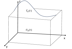
We will assume that the elastic structure at the top boundary of 𝒪\mathcal{O} displaces in only the transverse zz direction so that η\eta will be the time-dependent (scalar) displacement of the elastic structure from its reference configuration Γ\Gamma in the zz direction. Given a particular function η(t,x,y)\eta(t,x,y) describing the scalar transverse displacement of the elastic structure from Γ\Gamma, we can define the time-dependent fluid domain at time t[0,T]t\in[0,T] by (see Fig. 1):

(1) 𝒪η(t)={(x,y,z)3:(x,y)Γ,0z1+η(t,x,y)},\mathcal{O}_{\eta}(t)=\{(x,y,z)\in\mathbb{R}^{3}:(x,y)\in\Gamma,0\leq z\leq 1+\eta(t,x,y)\},

and the top boundary of 𝒪η(t)\mathcal{O}_{\eta}(t) will be the physical time-dependent configuration of the elastic structure at time tt, given by

(2) Γη(t)={(x,y,1+η(t,x,y):(x,y)Γ}.\Gamma_{\eta}(t)=\{(x,y,1+\eta(t,x,y):(x,y)\in\Gamma\}.

We will assume that a compressible, isentropic, viscous fluid occupies the three-dimensional domain 𝒪η(t)\mathcal{O}_{\eta}(t) at time tt and that the dynamics of the fluid and the structure influence each other.

Description of the fluid and structure subproblems. We now describe each of the subproblems separately.

For the fluid subproblem, we model the fluid velocity 𝒖{\boldsymbol{u}} and the fluid density ρ\rho by the compressible Navier-Stokes equations for a viscous fluid:

(3) {tρ+div(ρu)=0t(ρ𝒖)+div(ρ𝒖𝒖)𝝈(ρ,𝒖)=Ff on 𝒪η(t),\left\{\begin{array}[]{l}\partial_{t}\rho+\text{div}(\rho u)=0\\ \partial_{t}(\rho{\boldsymbol{u}})+\text{div}(\rho{\boldsymbol{u}}\otimes{\boldsymbol{u}})-\nabla\cdot\boldsymbol{\sigma}(\rho,{\boldsymbol{u}})=F_{f}\\ \end{array}\right.\quad\text{ on }\mathcal{O}_{\eta}(t),

where the Cauchy stress tensor 𝝈(ρ,𝒖)\boldsymbol{\sigma}(\rho,{\boldsymbol{u}}) is defined by

𝝈(ρ,𝒖)=2μ(𝑫(𝒖)13div(𝒖)𝑰)+(π+23μ)div(𝒖)𝑰p𝑰,\boldsymbol{\sigma}(\rho,{\boldsymbol{u}})=2\mu\left(\boldsymbol{D}({\boldsymbol{u}})-\frac{1}{3}\text{div}({\boldsymbol{u}})\boldsymbol{I}\right)+\left(\pi+\frac{2}{3}\mu\right)\text{div}({\boldsymbol{u}})\boldsymbol{I}-p\boldsymbol{I},

where 𝑫(𝒖)=12(𝒖+t𝒖)\displaystyle\boldsymbol{D}({\boldsymbol{u}})=\frac{1}{2}(\nabla{\boldsymbol{u}}+\nabla^{t}{\boldsymbol{u}}) is the symmetrized gradient of the velocity and FfF_{f} is an external force, to be specified later, which will eventually represent stochastic perturbations of the fluid momentum. Moreover, we assume that

λ=π+23μ>0.\lambda=\pi+\frac{2}{3}\mu>0.

The first equation is the continuity equation, which represents the conservation of mass, and the second equation represents the balance of momentum. Here, μ,λ>0\mu,\lambda>0 are the viscosity coefficients, and pp is the fluid pressure, which is given as a function of the fluid density ρ\rho through a constitutive relationship for the problem. In the current setting, we will assume that the viscous compressible fluid is isentropic so that the pressure law is given by a power law:

p(ρ)=ργ, for some positive constant γ>32.p(\rho)=\rho^{\gamma},\text{ for some positive constant }\gamma>\frac{3}{2}.

We prescribe periodic boundary condition for the fluid velocity in xx and yy direction and prescribe no-slip boundary condition on the bottom boundary i.e. 𝒖|Γb=0{\boldsymbol{u}}|_{\Gamma_{b}}=0.

For the structure subproblem, we model the evolution of the structure displacement η\eta by the Koiter shell equation:

(4) ttηαtΔη+Δ2η=Fs, on Γ,\partial_{tt}\eta-\alpha\partial_{t}\Delta\eta+\Delta^{2}\eta=F_{s},\qquad\text{ on }\Gamma,

where we recall that η\eta is the transverse scalar displacement in the zz direction of the elastic structure from its reference configuration Γ\Gamma. We emphasize that while the fluid equations are posed on the physical time-dependent domain, the elastodynamics of the structure are prescribed in the Eulerian coordinates on the reference domain. Here, the constant α\alpha represents a viscoelasticity parameter and we assume that α>0\alpha>0 in the current manuscript to obtain an existence result. We supply this elastodynamics equation for the structure displacement η\eta with periodic boundary conditions.

Description of the coupling conditions. We next couple these two subproblems together with the following coupling conditions, which are the kinematic coupling condition describing continuity of velocities and the dynamic coupling condition describing the load of the fluid on the elastodynamics of the structure:

  • The kinematic coupling condition describes the continuity of velocities via the no-slip condition along the moving (time-dependent) fluid-structure interface so that:

    (5) 𝒖=(tη)𝒆z on Γη(t),{\boldsymbol{u}}=(\partial_{t}\eta)\boldsymbol{e}_{z}\qquad\text{ on }\Gamma_{\eta}(t),

    where 𝒆z\boldsymbol{e}_{z} is the unit normal vector in the zz direction, and where we recall that the structure is assumed to displace in only the transverse zz direction.

  • The dynamic coupling condition describes the load of the fluid on the structure via the Cauchy stress tensor. This condition specifies the form of the external force on the structure as

    (6) Fs=𝝈(ρ,𝒖)𝒏(t)𝒆z+Fsstoch,F_{s}=-\boldsymbol{\sigma}(\rho,{\boldsymbol{u}})\boldsymbol{n}(t)\cdot\boldsymbol{e}_{z}+F_{s}^{stoch},

    where 𝒏(t)\boldsymbol{n}(t) is the time-dependent normal vector to the moving fluid-structure interface Γ(t)\Gamma(t), and where FsstochF_{s}^{stoch} is an external stochastic forcing acting on the structure that will be specified later.

Description of the maximal domain and the stochastic forcing. Next, we specify the nature of the stochastic forcing on the structure and the fluid. Let W1W_{1} and W2W_{2} be independent cylindrical Wiener processes in a separable Hilbert space 𝒰0\mathcal{U}_{0}. Letting {𝒆k}k=1\{\boldsymbol{e}_{k}\}_{k=1}^{\infty} be an orthonormal basis for 𝒰\mathcal{U}, we can consider a Wiener process to formally be the sum of βk(t)𝒆k\beta_{k}(t)\boldsymbol{e}_{k} over the positive integers kk, where βk\beta_{k} is a standard 1D Brownian motion. We will let the dynamics of the problem depend nonlinearly on the stochastic noise, as a function of the fluid density and the fluid momentum pointwise in the moving domain 𝒪η(t)\mathcal{O}_{\eta}(t).

Motivated by [7], we consider nonlinear noise intensity operators GG and 𝑭\boldsymbol{F} such that 𝑭(ρ,ρ𝒖):𝒰0Hl(3)\boldsymbol{F}(\rho,\rho{\boldsymbol{u}}):\mathcal{U}_{0}\to{H}^{-l}({\mathbb{R}}^{3}) for l>32l>\frac{3}{2} and G(η,v):𝒰0L2(Γ)G{(\eta,v)}:\mathcal{U}_{0}\to L^{2}(\Gamma) are Hilbert-Schmidt.  We define,

Ff=𝑭(ρ,ρ𝒖)dW1(t),Fs=G(η,v)dW2(t),F_{f}=\boldsymbol{F}(\rho,\rho{\boldsymbol{u}})dW_{1}(t),\qquad F_{s}=G(\eta,v)dW_{2}(t),

For given functions ρ:𝒪α\rho:\mathcal{O}_{\alpha}\to\mathbb{R} and 𝒖:𝒪α3{\boldsymbol{u}}:\mathcal{O}_{\alpha}\to\mathbb{R}^{3}, we define

fk(ρ,ρ𝒖,)=𝑭(ρ,ρ𝒖)𝒆k,gk(η,v,)=G(η,v)𝒆k.f_{k}(\rho,\rho{\boldsymbol{u}},\cdot)=\boldsymbol{F}(\rho,\rho{\boldsymbol{u}})\boldsymbol{e}_{k},\qquad g_{k}(\eta,v,\cdot)=G(\eta,v)\boldsymbol{e}_{k}.

We assume the following noise structure: There exists a sequence of positive constants {ck}k=1\{c_{k}\}_{k=1}^{\infty} with k=1ck2<\displaystyle\sum_{k=1}^{\infty}c_{k}^{2}<\infty such that for all positive integers kk, the functions fk:[0,)×3×3f_{k}:[0,\infty)\times{\mathbb{R}}^{3}\times{\mathbb{R}}^{3}\to{\mathbb{R}} and gk:××Γg_{k}:{\mathbb{R}}\times{\mathbb{R}}\times\Gamma\to{\mathbb{R}}, which are C1C^{1} functions in all of the inputs, satisfy:

(7) |fk(ρ,𝒒,x)|ck(ρ+|𝒒|),|ρ,𝒒fk(ρ,𝒒,x)|ck.\displaystyle|f_{k}(\rho,\boldsymbol{q},x)|\leq c_{k}(\rho+|\boldsymbol{q}|),\quad|\nabla_{\rho,\boldsymbol{q}}f_{k}(\rho,\boldsymbol{q},x)|\leq c_{k}.
(8) |gk(η,v,x)|ck(|η|+|v|),|η,vgk(η,v,x)|ck.\displaystyle|g_{k}(\eta,v,x)|\leq c_{k}(|\eta|+|v|),\quad|\nabla_{\eta,v}g_{k}(\eta,v,x)|\leq c_{k}.

Note in particular that (7) implies that the intensity of the noise in the momentum equations is identically zero whenever the fluid density is equal to zero which is consistent with deterministic theory. Moreover, this allows us to naturally extend the noise 𝑭dW\boldsymbol{F}dW outside of the moving domain to the entire space 3{\mathbb{R}}^{3} by assuming that the fluid density is equal to 0 outside of the moving domain.

2.1. Literature review

In this manuscript, we consider a stochastic model of fluid-structure interaction involving the coupled dynamics interaction between a viscous, compressible, isentropic fluid and a viscoelastic Koiter shell, perturbed by stochastic effects in both the fluid and structure elastodynamics. Problems involving compressible fluid dynamics and fluid-structure interaction in both the deterministic and stochastic settings have been of considerable interest in the past mathematical literature.

The mathematical study of existence of weak solutions to the (deterministic) compressible Navier-Stokes equations in 3{\mathbb{R}}^{3} goes back to the seminal work of P.-L. Lions in [29, 30], whose work first establishes the existence of weak solutions to the compressible Navier-Stokes equations where an isentropic compressible fluid is considered with a constitutive pressure law of p(ρ)=ργp(\rho)=\rho^{\gamma} for γ>9/5\gamma>9/5. These results were extended by another important work in [18], which uses a multilayer approximation scheme involving a Galerkin approximation along with artificial viscosity and artificial pressure to boost integrability of the pressure to establish existence of weak solutions for adiabatic constants γ>3/2\gamma>3/2, and this multilayer approximation scheme forms the basis for many existence results in the literature for systems involving compressible Navier-Stokes equations, including the one found in the current manuscript.

Analysis of compressible viscous fluid flows was later extended to the case of compressible fluid flows perturbed by stochastic (random in time) noise. Preliminary work in [43, 44] considered compressible Navier-Stokes equations in one spatial dimension with random perturbations, and work in higher dimensions was achieved first in [42] in two spatial dimensions and in [16] for three spatial dimensions with random noise of the form ρdW\rho dW, though the techniques presented in these two works are “semi-deterministic” in the sense that the weak formulation can be written without stochastic integrals using an appropriate transformation.

A subsequent fundamental work in the mathematical analysis of stochastic compressible fluid flows is [8], which studies the stochastic compressible Navier-Stokes equations with multiplicative noise. In this work, the existence of “finite energy weak martingale solutions” for stochastic isentropic compressible Navier-Stokes equations with adiabatic constant γ>3/2\gamma>3/2 is established following the aforementioned multilevel approximation scheme, but a new application of stochastic analysis techniques. Independently, another fundamental work in the analysis of such stochastic compressible flows is [37], which establishes global existence of weak martingale solutions for γ>9/5\gamma>9/5 for the 3D stochastic isentropic compressible Navier-Stokes, using a similar multilevel approximation, but also using a new application of a operator splitting technique (inspired by work in [2]), which separates the stochastic and deterministic components of the problem in a time-discretized splitting scheme.

The study of well-posedness for compressible flows was later extended to the study of coupled deterministic systems involving elastic structures and solids interacting dynamically with compressible viscous fluids, in the context of fluid-structure interaction (FSI). These models of compressible fluid-structure interaction are of two types: (1) immersed elastic bodies in a compressible viscous fluid, and (2) compressible viscous fluids interacting with shells, plates, or more generally, elastic structures of lower spatial dimension than the fluid domain (an example of which could be a compressible viscous fluid flowing through a tube with elastic walls).

For models of the first type involving immersed solids, work was first done for well-posedness of models involving rigid bodies immersed in surrounding barotropic compressible flows [4] and heat-conducting compressible flows [23]. Elastic bodies immersed in compressible flows were later considered, first in the context of higher order spatial derivative structure regularization of the structure elastodynamics [3] and later without this extra higher order spatial regularity in the elastodynamics equations [6]. These results were improved in terms of initial data regularity in the case of initial structue displacement being equal to zero in [27], and there were also extensions to nonlinearly elastic immersed solids in compressible viscous barotropic flows in the work of [5].

For models of the second type involving elastic structures of lower spatial dimension than the compressible fluid, one of the first works is [21], which features a 2D modified compressible Navier-Stokes equation with a linear pressure law interacting with a 1D elastic structure on the boundary of the fluid domain, and this work was later extended to the case of a 3D fluid domain [20] with modified isentropic compressible Navier-Stokes equations. The first analogue of the classical result by Feireisl [18] for existence of weak solutions to a deterministic compressible FSI model for γ>12/7\gamma>12/7 appears in [10], with the 3D compressible isentropic Navier-Stokes equations coupled to equations for a surrounding Koiter shell with the no-slip condition, where the compressible fluid equations posed on a time-dependent fluid domain that evolves depending on the a priori unknown displacement of the elastic Koiter shell on the boundary of the moving fluid domain, and these results were extended to the case of a similar compressible fluid-structure system with slip boundary conditions in [31]. These results were extended to the existence of weak solutions for the interaction between a heat-conducting compressible viscous fluid and an elastic Koiter shell with the no-slip condition in [11] and the interaction between a heat-conducting compressible viscous fluid and a thermoelastic shell with the no-slip condition in [32]. We also remark that there has also been a recent result on existence of strong solutions to a 2D model of compressible isentropic viscous Navier-Stokes equations interacting with a viscoelastic beam for sufficiently regular initial data with initial displacement equal to zero in [34].

All of the aforementioned works described have been in the context of deterministic dynamics, and we make hence make some general comments about the literature relating to the study of stochastic fluid-structure systems in general. The study of stochastic coupled fluid-structure dynamics is relatively new, and until the present work, has exclusively involved incompressible viscous fluids, rather than compressible viscous fluids. Work on stochastic incompressible fluid-structure interaction began first with a fully coupled model [26] involving the coupled interaction between the linear Stokes equations and a wave equation with external additive stochastic structure forcing. The problem considered in this paper is linearly coupled in the sense that the movement of the structure displacement is “linearized” and the fluid equations are posed on a fixed reference domain. These results were then extended to the more challenging case of stochastic incompressible fluid-structure interaction involving the Navier-Stokes equations interacting with an elastic shell, with multiplicative stochastic forcing acting on both the fluid/structure in [40], where the existence of weak martingale solutions is established. The well-posedness of an analogous moving-boundary stochastic model was also established in the different context of noise of transport type perturbing the structure elastodynamics [9]. Later, existence of weak martingale solutions to stochastic coupled moving boundary systems of incompressible Navier-Stokes equations interacting with elastic shells was established for more general models, including models with unrestricted structure displacements [38] and models with more general Navier-slip boundary conditions [39].

We emphasize that so far, the past mathematical literature on stochastic fluid-structure dynamics has been restricted the study of incompressible fluids. Hence, the goal of the current manuscript is to extend the study of stochastic fluid-structure interaction to the compressible regime.

3. Weak martingale solutions and the main result

Definition 3.1 (Definition of a weak martingale solution).

Let the deterministic initial structure configuration η0H2(Γ)\eta_{0}\in H^{2}(\Gamma) be such that for some α0>0\alpha_{0}>0 we have,

(9) α0<1+η0(z),zΓ, and η0H2(Γ)<1α0.\displaystyle\alpha_{0}<1+\eta_{0}(z),\quad\forall z\in\Gamma,\quad\text{ and }\quad{\|\eta_{0}\|_{H^{2}(\Gamma)}<\frac{1}{\alpha_{0}}}.

Let ρ0Lγ(𝒪η0)\rho_{0}\in L^{\gamma}({\mathcal{O}}_{\eta_{0}}) and v0L2(Γ)v_{0}\in L^{2}(\Gamma) be given deterministic initial data. Assume that when ρ0>0\rho_{0}>0, given 𝒑0\boldsymbol{p}_{0} satisfies |𝒑0|2ρ0L1(𝒪η0)\frac{|\boldsymbol{p}_{0}|^{2}}{\rho_{0}}\in L^{1}({\mathcal{O}}_{\eta_{0}}). We say that (𝒮,ρ,𝒖,η,τ)(\mathscr{S},\rho,{\boldsymbol{u}},\eta,\tau) is a martingale solution to the system (3)-(6) if:

  1. (1)

    𝒮=(Ω,,(t)t0,,W1,W2)\mathscr{S}=(\Omega,\mathcal{F},(\mathcal{F}_{t})_{t\geq 0},{\mathbb{P}},W_{1},W_{2}) is a stochastic basis, that is, (Ω,,(t)t0,)(\Omega,\mathcal{F},(\mathcal{F}_{t})_{t\geq 0},{\mathbb{P}}) is a filtered probability space satisfying the usual conditions and W1W_{1} and W2W_{2} are independent 𝒰\mathcal{U}-valued (t)t0(\mathcal{F}_{t})_{t\geq 0}-Wiener processes.

  2. (2)

    ηL2(Ω;L(0,T;H2(Γ))W1,(0,T;L2(Γ))H1(0,T;H1(Γ)))\eta\in L^{2}(\Omega;L^{\infty}(0,T;H^{2}(\Gamma))\cap W^{1,\infty}(0,T;L^{2}(\Gamma)){{\cap H^{1}(0,T;H^{1}(\Gamma))}})

  3. (3)

    𝒖L(0,T;L2(𝒪η()))L2(0,T;W1,p(𝒪η())){\boldsymbol{u}}\in L^{\infty}(0,T;L^{2}({\mathcal{O}}_{\eta}(\cdot)))\cap L^{2}(0,T;W^{1,p}({\mathcal{O}}_{\eta}(\cdot))) and ρL(0,T;Lγ(𝒪η()))\rho\in L^{\infty}(0,T;L^{\gamma}({\mathcal{O}}_{\eta}(\cdot))) {\mathbb{P}}-almost surely.

  4. (4)

    τ\tau is a {\mathbb{P}}-almost surely strictly positive (t)t0(\mathcal{F}_{t})_{t\geq 0}-stopping time;

  5. (5)

    The random distributions ρ,𝒖,tη,\rho,{\boldsymbol{u}},\partial_{t}\eta, and the stochastic process η\eta, are (t)t0(\mathcal{F}_{t})_{t\geq 0}-progressively measurable.

  6. (6)

    The renormalized continuity equation holds {\mathbb{P}}-almost surely:

    (10) 0t𝒪η(t)b(ρ)(tϕ+𝒖ϕ)=0t𝒪η(t)(b(ρ)ρb(ρ))(𝒖)ϕ+𝒪η0ρ0b(ρ0)ϕ(0),\displaystyle\int_{0}^{t}\int_{{\mathcal{O}}_{\eta}(t)}b(\rho)(\partial_{t}\phi+{\boldsymbol{u}}\cdot\nabla\phi)=\int_{0}^{t}\int_{{\mathcal{O}}_{\eta}(t)}(b^{\prime}(\rho)\rho-b(\rho))(\nabla\cdot{\boldsymbol{u}})\phi+\int_{{\mathcal{O}}_{\eta_{0}}}\rho_{0}b(\rho_{0})\phi(0),

    for any essentially bounded process ϕ\phi taking values in C0([0,T)×𝒪¯η())C^{\infty}_{0}([0,T)\times\bar{\mathcal{O}}_{\eta}(\cdot)) and bC()b\in C({\mathbb{R}}) with b(z)=0b^{\prime}(z)=0 when zMbz\geq M_{b}.

  7. (7)

    For every (t)t0(\mathcal{F}_{t})_{t\geq 0}-adapted, essentially bounded smooth process (𝒒,ψ)({\boldsymbol{q}},\psi) such that 𝒒|Γη=ψ{\boldsymbol{q}}|_{\Gamma_{\eta}}=\psi, {\mathbb{P}}-almost surely, the following equation holds for {\mathbb{P}}-almost surely, for almost every t[0,τ)t\in[0,\tau):

    (11) 𝒪η(t)ρ(t)𝒖(t)𝒒(t)𝑑𝐱+Γtη(t)ψ(t)dz=𝒪η0𝒑0𝒒(0)𝑑𝐱+Γv0ψ(0)𝑑𝒛+0t𝒪η(t)ρ𝒖t𝒒d𝐱dt+0t𝒪η(t)ρ𝒖𝒖:𝒒d𝐱dt2μ0t𝒪η(t)𝒖:𝒒d𝐱dt+0t𝒪η(t)ργ(𝒒)𝑑𝐱𝑑tλ0t𝒪η(t)div(𝒖)div(𝒒)𝑑𝐱𝑑t+0tΓtηtψd𝒛dt0tΓtηψd𝒛dt0tΓ(ηψ+ΔηΔψ)𝑑𝒛𝑑t+0t𝒪η(t)F(ρ,ρ𝒖)𝒒𝑑W1(t)+0tΓG(η,tη)ψ𝑑W2(t).\begin{split}&{\int_{{\mathcal{O}}_{\eta}(t)}\rho(t){\boldsymbol{u}}(t)\cdot{\boldsymbol{q}}(t)d{\bf x}+\int_{\Gamma}\partial_{t}\eta(t)\psi(t)dz}=\int_{{\mathcal{O}}_{\eta_{0}}}\boldsymbol{p}_{0}\cdot{\boldsymbol{q}}(0)d{\bf x}+\int_{\Gamma}v_{0}\psi(0)d\boldsymbol{z}\\ &+\int_{0}^{t}\int_{{\mathcal{O}}_{\eta}(t)}\rho{\boldsymbol{u}}\cdot\partial_{t}{\boldsymbol{q}}d{\bf x}dt+\int_{0}^{t}\int_{{\mathcal{O}}_{\eta}(t)}\rho{\boldsymbol{u}}\otimes{\boldsymbol{u}}:\nabla{\boldsymbol{q}}d{\bf x}dt-2\mu\int_{0}^{t}\int_{{\mathcal{O}}_{\eta}(t)}\nabla{\boldsymbol{u}}:\nabla{\boldsymbol{q}}d{\bf x}dt\\ &+\int_{0}^{t}\int_{{\mathcal{O}}_{\eta}(t)}\rho^{\gamma}(\nabla\cdot{\boldsymbol{q}})d{\bf x}dt-\lambda\int_{0}^{t}\int_{{\mathcal{O}}_{\eta}(t)}\text{div}({\boldsymbol{u}})\text{div}({\boldsymbol{q}})d{\bf x}dt\\ &+\int_{0}^{t}\int_{\Gamma}\partial_{t}\eta\partial_{t}\psi d\boldsymbol{z}dt-{\int_{0}^{t}\int_{\Gamma}\nabla\partial_{t}\eta\cdot\nabla\psi d\boldsymbol{z}dt-\int_{0}^{t}\int_{\Gamma}(\nabla\eta\nabla\psi+\Delta\eta\Delta\psi)d\boldsymbol{z}dt}\\ &+\int_{0}^{t}\int_{{\mathcal{O}}_{\eta}(t)}F(\rho,\rho{\boldsymbol{u}})\cdot{\boldsymbol{q}}\,dW_{1}(t)+\int_{0}^{t}\int_{\Gamma}G(\eta,\partial_{t}\eta)\psi dW_{2}(t).\end{split}
  8. (8)

    The kinematic coupling condition holds: 𝒖|Γη=tη𝐞z{\boldsymbol{u}}|_{\Gamma_{\eta}}=\partial_{t}\eta{\bf e}_{z}, {\mathbb{P}}-almost surely.

We are now in position to state the main result of this paper.

Theorem 3.1.

Let the initial deterministic structure configuration η0H2(Γ)\eta_{0}\in H^{2}(\Gamma) be such that for some α>0\alpha>0, we have:

(12) α<1+η0(z),zΓ, and 1+η0H2(Γ)<1α.\displaystyle{\alpha<1+\eta_{0}(z),\quad\forall z\in\Gamma,\quad\text{ and }\quad{\|1+\eta_{0}\|_{H^{2}(\Gamma)}<\frac{1}{\alpha}}.}

Consider deterministic initial data, consisting of an initial density ρ0Lγ(𝒪η0)\rho_{0}\in L^{\gamma}(\mathcal{O}_{\eta_{0}}) with ρ00\rho_{0}\geq 0, an initial momentum 𝒑0L2γγ+1(𝒪η0)\boldsymbol{p}_{0}\in L^{\frac{2\gamma}{\gamma+1}}({\mathcal{O}}_{\eta_{0}}) such that 𝒑0\boldsymbol{p}_{0} vanishes whenever ρ0\rho_{0} vanishes and |𝒑0|2ρ0L1(𝒪η0)\frac{|\boldsymbol{p}_{0}|^{2}}{\rho_{0}}\in L^{1}({\mathcal{O}}_{\eta_{0}}) (where this quotient is defined to be zero when ρ0\rho_{0} vanishes), and an initial structure velocity v0L2(Γ)v_{0}\in L^{2}(\Gamma). Assume that the noise coefficients FF and GG satisfy the growth conditions (7)-(8). Then there exists at least one martingale solution to the system (3)-(6) in the sense of Definition 3.1.

4. The approximation scheme

Before presenting our splitting scheme in Section 4.3, we will present the necessary setup. We fix some parameter α>0\alpha>0, which will be the parameter for which the approximate structure displacements we work with at all steps of the existence proof will satisfy ηHs(Γ)1α\|\eta\|_{H^{s}(\Gamma)}\leq\frac{1}{\alpha}, for some s(3/2,2)s\in(3/2,2). Since s(3/2,2)s\in(3/2,2), by Sobolev embedding of Hs(Γ)C(Γ)H^{s}(\Gamma)\subset C(\Gamma), this allows us to define a maximal domain 𝒪α\mathcal{O}_{\alpha}:

𝒪α={(x,y,z)3:(x,y)Γ,0z2+α1}.\mathcal{O}_{\alpha}=\{(x,y,z)\in\mathbb{R}^{3}:(x,y)\in\Gamma,0\leq z\leq 2+\alpha^{-1}\}.

4.1. Extension to the maximal domain

Because we are extending the problem from the physical moving domain to a fixed maximal domain, we will need to extend both the viscosity coefficients and initial data to the maximal domain 𝒪α\mathcal{O}_{\alpha}. We first consider the extension of the viscosity coefficients from the time-dependent domain 𝒪η(t){\mathcal{O}}_{\eta}(t) to the maximal domain 𝒪α\mathcal{O}_{\alpha}, and for this, it is useful to define smooth bounding functions aκηa^{\eta}_{\kappa} and bκηb^{\eta}_{\kappa} with aκη>η>bκηa^{\eta}_{\kappa}>\eta>b^{\eta}_{\kappa}, which define a tubular neighborhood (with width controlled by the parameter κ\kappa) around a given physical structure location determined by the displacement η\eta. The bounding functions aκηa^{\eta}_{\kappa} will be useful for the extension of viscosity coefficients, and both bounding functions aκηa^{\eta}_{\kappa} and bκηb^{\eta}_{\kappa} will also be useful later for the construction of test functions in Section 8.3.

Definition of the bounding functions. We now define the bounding functions aκηa^{\eta}_{\kappa} and bκηb^{\eta}_{\kappa}. Given a structure displacement ηHs(Γ)C(Γ)\eta\in H^{s}(\Gamma)\subset C(\Gamma) with ηHs(Γ)α\|\eta\|_{H^{s}(\Gamma)}\leq\alpha for some s(3/2,2)s\in(3/2,2), there exists CαC_{\alpha} (depending only on α\alpha) such that

(13) |η(w1)η(w2)|Cα|w1w2|1/2, for all w1,w2Γ.|\eta(w_{1})-\eta(w_{2})|\leq C_{\alpha}|w_{1}-w_{2}|^{1/2},\quad\text{ for all }w_{1},w_{2}\in\Gamma.

Given an extension parameter κ\kappa, we use this 1/21/2-Hölder continuity constant CαC_{\alpha} to define

ηκ(x,y)=η(x,y)+2Cακ1/2,ηκ(x,y)=η(x,y)2Cακ1/2,\eta^{\sharp}_{\kappa}(x,y)=\eta(x,y)+2C_{\alpha}\kappa^{1/2},\quad\eta^{\flat}_{\kappa}(x,y)=\eta(x,y)-2C_{\alpha}\kappa^{1/2},

and to define the smooth bounding functions

(14) aκη=1+(ηκζκ),bκη=1(ηκζκ),a^{\eta}_{\kappa}=1+(\eta^{\sharp}_{\kappa}*\zeta_{\kappa}),\quad\quad b^{\eta}_{\kappa}=1-(\eta^{\flat}_{\kappa}*\zeta_{\kappa}),

where ζκ=κ2ζ(κ1)\zeta_{\kappa}=\kappa^{-2}\zeta(\kappa^{-1}\cdot) is the usual smooth convolution kernel in 2{\mathbb{R}}^{2} with support in a ball of radius κ\kappa, and where the functions ηκ\eta^{\sharp}_{\kappa} and ηκ\eta^{\flat}_{\kappa} are extended by a constant outside of Γ\Gamma in order to define the convolution. We observe that

(15) aκη>1+η>bκη,a^{\eta}_{\kappa}>1+\eta>b^{\eta}_{\kappa},

since given (x,y)Γ(x,y)\in\Gamma, for all |w(x,y)|κ|w-(x,y)|\leq\kappa, we have that ηκ(w)>η(z)\eta^{\sharp}_{\kappa}(w)>\eta(z) and ηκ(w)<η(z)\eta^{\flat}_{\kappa}(w)<\eta(z) by (13). Furthermore, the estimate (13) also implies that

|(ηκζκ)(w)ηκ(w)|Cακ1/2,|(ηκζκ)(w)ηκ(w)|Cακ1/2,|(\eta^{\sharp}_{\kappa}*\zeta_{\kappa})(w)-\eta^{\sharp}_{\kappa}(w)|\leq C_{\alpha}\kappa^{1/2},\quad|(\eta^{\flat}_{\kappa}*\zeta_{\kappa})(w)-\eta^{\flat}_{\kappa}(w)|\leq C_{\alpha}\kappa^{1/2},

and hence:

(16) Cακ1/2aκη(w)(1+η(w))3Cακ1/2,C_{\alpha}\kappa^{1/2}\leq a^{\eta}_{\kappa}(w)-(1+\eta(w))\leq 3C_{\alpha}\kappa^{1/2},
(17) Cακ1/2(1+η(w))bκη(w)3Cακ1/2.C_{\alpha}\kappa^{1/2}\leq(1+\eta(w))-b^{\eta}_{\kappa}(w)\leq 3C_{\alpha}\kappa^{1/2}.

Extension of viscosity coefficients. We will use the bounding function aκηa^{\eta}_{\kappa} to extend the viscosity coefficients from the physical fluid domain to the fixed maximal domain 𝒪α\mathcal{O}_{\alpha} via an extension map. To define this extension map, we consider a smooth function ϕκ:\phi_{\kappa}:{\mathbb{R}}\to{\mathbb{R}} such that ϕκ(w)=1\phi_{\kappa}(w)=1 when w14w\leq\frac{1}{4}, ϕκ\phi_{\kappa} is decreasing on [14,34][\frac{1}{4},\frac{3}{4}], and ϕκ(w)=κ\phi_{\kappa}(w)=\kappa for w34w\geq\frac{3}{4}. Then, given ηHs(Γ)\eta\in H^{s}(\Gamma) for s(3/2,2)s\in(3/2,2), we can define an extension operator by defining χκη\chi^{\eta}_{\kappa} to be a smooth compactly supported function on [0,1]2×[0,)[0,1]^{2}\times[0,\infty), given by

(18) χκη(x,y,z)=ϕκ(zaκη(x,y)κ1/2).\chi^{\eta}_{\kappa}(x,y,z)=\phi_{\kappa}\left(\frac{z-a^{\eta}_{\kappa}(x,y)}{\kappa^{1/2}}\right).

For an appropriately chosen value of κ\kappa, χκη\chi_{\kappa}^{\eta} will be used to extend the viscosity parameters μ\mu and λ\lambda (31) in the fluid sub-problem (LABEL:fluidsubproblem).

Extension and approximation of the initial data. Recall that we are given deterministic initial data for the fluid density ρ0Lγ(𝒪α)\rho_{0}\in L^{\gamma}(\mathcal{O}_{\alpha}) and the fluid momentum 𝒑0L2γγ+1(𝒪α)\boldsymbol{p}_{0}\in L^{\frac{2\gamma}{\gamma+1}}(\mathcal{O}_{\alpha}) defined on the initial moving fluid domain 𝒪η0\mathcal{O}_{\eta_{0}}, so we must extend the initial data to the maximal domain 𝒪α\mathcal{O}_{\alpha}. We must perform this extension of the initial data to the maximal domain 𝒪α\mathcal{O}_{\alpha} carefully, as we will initially need the fluid density to be bounded below by some positive constant in order to apply a comparison principle to obtain existence of first-level approximate solutions, but in a final limit passage (which will later correspond to sending a parameter δ0\delta\to 0), we will require the initial density to vanish outside the initial physical fluid domain. So we use two layers of approximation of the initial data, with two parameters ε>0\varepsilon>0 and δ>0\delta>0, where the following approximations of the initial data are motivated by techniques found in the beginning of Section 4 of [18], and (3.6)-(3.8) in [32].

First, we extend the initially given deterministic initial data ρ0\rho_{0} and 𝒑0\boldsymbol{p}_{0} on 𝒪η0\mathcal{O}_{\eta_{0}} by zero to get initial data on 𝒪α\mathcal{O}_{\alpha}. For each parameter δ>0\delta>0, we approximate this initial data by a pair (ρ0,δ,𝒑0,δ)(\rho_{0,\delta},\boldsymbol{p}_{0,\delta}), where ρ0,δC2+ν(𝒪α)\rho_{0,\delta}\in C^{2+\nu}(\mathcal{O}_{\alpha}) satisfying

0ρ0,δδ1/β,ρ0,δ|𝒪α𝒪η0=0,limδ0|{ρ0,δ<ρ0}|0,ρ0,δρ0 in Lγ(𝒪α),\displaystyle 0\leq\rho_{0,\delta}\leq\delta^{-1/\beta},\quad\rho_{0,\delta}|_{\mathcal{O}_{\alpha}\setminus\mathcal{O}_{\eta_{0}}}=0,\quad\lim_{\delta\to 0}|\{\rho_{0,\delta}<\rho_{0}\}|\to 0,\quad\rho_{0,\delta}\to\rho_{0}\text{ in }L^{\gamma}(\mathcal{O}_{\alpha}),
(19) 𝒑0,δ=𝒑0, if ρ0,δρ0,𝒑0=𝟎 otherwise.\displaystyle\boldsymbol{p}_{0,\delta}=\boldsymbol{p}_{0},\text{ if }\rho_{0,\delta}\geq\rho_{0},\quad\boldsymbol{p}_{0}=\boldsymbol{0}\text{ otherwise.}

These properties imply that the modified energy 12𝒪α|𝒑0,δ|2ρ0,δ+aγ1𝒪αρ0,δγ+δβ1𝒪αρ0,δβ\displaystyle\frac{1}{2}\int_{\mathcal{O}_{\alpha}}\frac{|\boldsymbol{p}_{0,\delta}|^{2}}{\rho_{0,\delta}}+\frac{a}{\gamma-1}\int_{\mathcal{O}_{\alpha}}\rho_{0,\delta}^{\gamma}+\frac{\delta}{\beta-1}\int_{\mathcal{O}_{\alpha}}\rho_{0,\delta}^{\beta} is uniformly bounded independently of δ\delta, and that 𝒑0,δ𝒑0\boldsymbol{p}_{0,\delta}\to\boldsymbol{p}_{0} in L2γγ+1(𝒪α)L^{\frac{2\gamma}{\gamma+1}}(\mathcal{O}_{\alpha}).

For the next layer of approximation involving the parameter ε>0\varepsilon>0 for fixed but arbitrary δ>0\delta>0, we choose ρ0,δ,εC2+ν(𝒪α)\rho_{0,\delta,\varepsilon}\in C^{2+\nu}(\mathcal{O}_{\alpha}) such that

(20) 0<ερ0,δ,εδ1/β,ρ0,δ,ερ0,δ in Lγ(𝒪α),0<\varepsilon\leq\rho_{0,\delta,\varepsilon}\leq\delta^{-1/\beta},\quad\rho_{0,\delta,\varepsilon}\to\rho_{0,\delta}\text{ in $L^{\gamma}(\mathcal{O}_{\alpha})$},

and the initial fluid momentum 𝒑0,δ,ε\boldsymbol{p}_{0,\delta,\varepsilon}, using the argument in the beginning of Section 4 in [18] and the beginning of Section 6 in [8], can be chosen to satisfy

|𝒑0,δ,ε|2ρ0,δ,ε is uniformly bounded (independently of ε) in L1(𝒪α),\displaystyle\frac{|\boldsymbol{p}_{0,\delta,\varepsilon}|^{2}}{\rho_{0,\delta,\varepsilon}}\text{ is uniformly bounded (independently of $\varepsilon$) in $L^{1}(\mathcal{O}_{\alpha})$},
𝒑0,δ,ε𝒑0,δ in L1(𝒪α),𝒑0,δ,ερ0,δ,ε𝒑0,δρ0,δ in L2(𝒪α), as ε0.\displaystyle\boldsymbol{p}_{0,\delta,\varepsilon}\to\boldsymbol{p}_{0,\delta}\text{ in }L^{1}(\mathcal{O}_{\alpha}),\quad\frac{\boldsymbol{p}_{0,\delta,\varepsilon}}{\sqrt{\rho_{0,\delta,\varepsilon}}}\to\frac{\boldsymbol{p}_{0,\delta}}{\sqrt{\rho_{0,\delta}}}\text{ in }L^{2}(\mathcal{O}_{\alpha}),\quad\text{ as $\varepsilon\to 0$.}

We remark that the modified energy 12𝒪α|𝒑0,δ,ε|2ρ0,δ,ε+aγ1𝒪αρ0,δ,εγ+δβ1𝒪αρ0,δ,εβ\displaystyle\frac{1}{2}\int_{\mathcal{O}_{\alpha}}\frac{|\boldsymbol{p}_{0,\delta,\varepsilon}|^{2}}{\rho_{0,\delta,\varepsilon}}+\frac{a}{\gamma-1}\int_{\mathcal{O}_{\alpha}}\rho_{0,\delta,\varepsilon}^{\gamma}+\frac{\delta}{\beta-1}\int_{\mathcal{O}_{\alpha}}\rho_{0,\delta,\varepsilon}^{\beta} is similarly bounded uniformly, independently of ε\varepsilon and δ\delta.

Given the extended initial data (ρ0,δ,ε,𝒑0,δ,ε)(\rho_{0,\delta,\varepsilon},\boldsymbol{p}_{0,\delta,\varepsilon}) on the maximal domain 𝒪α\mathcal{O}_{\alpha}, our splitting scheme will include extension of the fluid equations to the larger domain 𝒪α\mathcal{O}_{\alpha}, by penalizing the kinematic coupling condition via the parameter δ>0\delta>0. While this extension seems unnatural at this stage, we will eventually prove that the fluid momentum exists only in the time-dependent moving domain by proving that its density vanishes outside as δ0\delta\to 0 (cf. Proposition 8.4) thus retrieving the original formulation on the moving domain.

4.2. Description of the Galerkin approximation.

Let {𝝍i}i=1\{\boldsymbol{\psi}_{i}\}_{i=1}^{\infty} be an orthonormal basis for L2(𝒪α)L^{2}(\mathcal{O}_{\alpha}) and an orthogonal basis for Hl(𝒪α){H^{l}(\mathcal{O}_{\alpha})} for l>5/2l>5/2, and let {ξi}i=1\{\xi_{i}\}_{i=1}^{\infty} be an orthonormal basis for L2(Γ)L^{2}(\Gamma) and an orthogonal basis for H2(Γ)H^{2}(\Gamma). Define

(21) Xnf:=span{ψ1,ψ2,,ψn}Hl(𝒪α),X_{n}^{f}:=\text{span}\{\psi_{1},\psi_{2},...,\psi_{n}\}\subset H^{l}(\mathcal{O}_{\alpha}),
(22) Xnst:=span{φ1,φ2,,φn}H2(Γ),X_{n}^{{st}}:=\text{span}\{{\varphi_{1},\varphi_{2},...,\varphi_{n}}\}\subset H^{2}(\Gamma),

where XnfX_{n}^{f} is endowed with the L2(𝒪α)L^{2}(\mathcal{O}_{\alpha}) inner product and XnstX_{n}^{st} is endowed with the L2(Γ)L^{2}(\Gamma) inner product. Define

(23) Xn:=Xnf×XnstX_{n}:=X_{n}^{f}\times X_{n}^{st}

to be the full fluid-structure Galerkin space with the usual product norm. Let Pnf:L2(𝒪α)XnfP^{f}_{n}:L^{2}(\mathcal{O}_{\alpha})\to X^{f}_{n} be the orthogonal projection operator from L2(𝒪α)L^{2}(\mathcal{O}_{\alpha}) onto XnfX^{f}_{n} and let Pnst:L2(Γ)XnstP^{st}_{n}:L^{2}(\Gamma)\to X^{st}_{n} be the orthogonal projection operator from L2(Γ)L^{2}(\Gamma) onto XnstX^{st}_{n}. Let (Xnf)(X_{n}^{f})^{*} and (Xnst)(X_{n}^{st})^{*} denote the dual spaces of linear functionals on XnfX^{f}_{n} and XnstX^{st}_{n} respectively. We remark that the choice of the function space Hl(𝒪α)H^{l}(\mathcal{O}_{\alpha}) for l>5/2l>5/2 is compatible with the comparison principle for the continuity equation with viscosity stated in (39), as functions in Hl(𝒪α)H^{l}(\mathcal{O}_{\alpha}) have divergences that are in L(𝒪α)L^{\infty}(\mathcal{O}_{\alpha}) by standard Sobolev embedding in three spatial dimensions.

4.3. The operator splitting scheme

Upon defining the problem on the extended domain 𝒪α\mathcal{O}_{\alpha}, we will then use a splitting scheme to construct approximate solutions defined on a fixed time interval [0,T][0,T], where TT will be a fixed, but arbitrary final time. We will use an operator splitting scheme that divides the entire time interval [0,T][0,T] for a parameter NN into NN subintervals [tj,tj+1][t_{j},t_{j+1}] of length Δt\Delta t. For each j=1,2,,N1j=1,2,...,N-1, we will run decoupled structure and fluid subproblems to update all of these approximate quantities on [tj,tj+1][t_{j},t_{j+1}]

We will keep track of four approximate solution quantities defined continuously in time on [0,T][0,T]: the fluid density ρN\rho_{N}, the fluid velocity 𝒖N{\boldsymbol{u}}_{N}, the structure displacement ηN\eta_{N}, and the structure velocity vNv_{N}. In addition, we will have a “stopped” process ηN\eta^{*}_{N}, which is the structure displacement stopped at the first time of leaving desired bounds on the displacement of the structure.

The structure subproblem. We update the structure displacement by solving the following weak formulation for ηNL2(Ω;W1,(tj,tj+1;Xnst)))\eta_{N}\in L^{2}(\Omega;W^{1,\infty}(t_{j},t_{j+1};X_{n}^{st}))) for the Galerkin space XnstX_{n}^{st} defined in (22):

(24) jΔt(j+1)ΔtΓηNψjΔt(j+1)ΔtΓΔηNΔψjΔt(j+1)ΔtΓtηNψ1δjΔt(j+1)ΔtT𝒯ΔtηNδ(tηN𝒆zτΔt𝒖N)ψ𝒆z+jΔt(j+1)ΔtΓGn(ηN,tηN)ψ𝑑W2(t)=jΔt(j+1)Δtddt(ΓtηNψ),\begin{split}&-\int_{j\Delta t}^{(j+1)\Delta t}\int_{\Gamma}\nabla\eta_{N}\cdot\nabla\psi-\int_{j\Delta t}^{(j+1)\Delta t}\int_{\Gamma}\Delta\eta_{N}\Delta\psi-\int_{j\Delta t}^{(j+1)\Delta t}\int_{\Gamma}\nabla\partial_{t}\eta_{N}\cdot\nabla\psi\\ &-\frac{1}{\delta}\int_{j\Delta t}^{(j+1)\Delta t}\int_{T^{\delta}_{\mathcal{T}_{\Delta t}\eta^{*}_{N}}}(\partial_{t}\eta_{N}\boldsymbol{e}_{z}-\tau_{\Delta t}{\boldsymbol{u}}_{N})\cdot\psi\boldsymbol{e}_{z}\\ &+\int_{j\Delta t}^{(j+1)\Delta t}\int_{\Gamma}G_{n}(\eta_{N},\partial_{t}\eta_{N})\psi dW_{2}(t)=\int_{j\Delta t}^{(j+1)\Delta t}\frac{d}{dt}\left(\int_{\Gamma}\partial_{t}\eta_{N}\psi\right),\end{split}

holds {\mathbb{P}}-almost surely for every spatial test function ψXnst\psi\in X_{n}^{st}. Here the noise coefficient is

(25) Gn:=PnstGG_{n}:=P^{st}_{n}G

and the time shifts are 𝒯Δtf=f(tΔt)\mathcal{T}_{\Delta t}f=f\left(t-{\Delta t}\right). The penalty term that decouples the structure equations from the momentum equation is defined on the tubular neighborhood: TηδT^{\delta}_{\eta} is the tubular neighborhood

(26) Tηδ:={(x,y,z)𝒪α𝒪η:0<(z1η)<δ(121β)}.\displaystyle T^{\delta}_{\eta}:=\{(x,y,z)\in{\mathcal{O}}_{\alpha}\setminus{\mathcal{O}}_{\eta}:0<(z-1-\eta)<\delta^{(\frac{1}{2}-\frac{1}{\beta})}\}.

Finally, the so-called artificial structure displacement is the following stopped process:

(27) ηN(t)=ηN(τNηt),\eta^{*}_{N}(t)=\eta_{N}(\tau^{\eta}_{N}\wedge t),

where for a fixed s(3/2,2)s\in(3/2,2), the stopping time τNη\tau^{\eta}_{N} is defined as follows:

τNη\displaystyle\tau^{\eta}_{N} :=Tinf{t>0:infΓ(1+ηN(t,))<α or ηN(t,)Hs(Γ)1α}.\displaystyle:=T\wedge\inf\left\{t>0:\inf_{\Gamma}(1+{\eta_{N}}(t,\cdot))<\alpha\text{ or }\|{\eta}_{N}(t,\cdot)\|_{H^{s}(\Gamma)}\leq\frac{1}{\alpha}\right\}.
Refer to caption
Figure 2. Graphs of functions bounding any structure displacement

The reason behind using this stopped processes, which will stop the process ηN\eta_{N} at the first time at which the approximate solution leaves the desired bounds, indicated by the parameter α>0\alpha>0, is because we want to avoid self-collision and want to be able to define the fluid subproblem by extending it to a fixed bounded domain. Because ηNC(0,T;Hs(Γ))C(0,T;C(Γ))\eta_{N}\in C(0,T;H^{s}(\Gamma))\subset C(0,T;C(\Gamma)) for any s(3/2,2)s\in(3/2,2), this is indeed a stopping time.

Then on [tj,tj+1][t_{j},t_{j+1}] we set

vN(t)=tηN,v_{N}(t)=\partial_{t}\eta_{N},

where this time derivative is interpreted as a weak derivative.

We use the stopped structure displacement ηN\eta^{*}_{N} because this allows us to define the splitting scheme (in particular for the fluid subproblem) on the entire time interval [0,T][0,T], as we can use ηN\eta^{*}_{N} to define a moving fluid domain that does not exhibit domain degeneracies on the whole time interval [0,T][0,T]. However, we emphasize the important point that in order to obtain uniform estimates on [0,T][0,T] for the structure elastodynamics, we do not stop the structure subproblem at the stopping time τNη(t)\tau^{\eta}_{N}(t) and instead continue to update and evolve the structure displacement all the way until the final time TT.

The fluid subproblem. For the fluid subproblem on the interval [tj,tj+1][t_{j},t_{j+1}], we will solve for the fluid density and velocity

ρNL2(Ω;L(tj,tj+1;Lβ(𝒪α))),𝒖NL2(Ω;L2(tj,tj+1;H1(𝒪α))),\rho_{N}\in L^{2}(\Omega;L^{\infty}(t_{j},t_{j+1};L^{\beta}(\mathcal{O}_{\alpha}))),\qquad{\boldsymbol{u}}_{N}\in L^{2}(\Omega;L^{2}(t_{j},t_{j+1};H^{1}(\mathcal{O}_{\alpha}))),

so that the weak formulation of the continuity equation holds for all smooth test functions φCc(𝒪¯α)\varphi\in C_{c}^{\infty}(\overline{\mathcal{O}}_{\alpha}):

𝒪αρN(tj+1)φ\displaystyle\int_{\mathcal{O}_{\alpha}}\rho_{N}(t_{j+1})\varphi =𝒪αρN(tj)φ+2tjtj+1𝒪αρN𝒖Nφ2εtjtj+1𝒪αρNφ,\displaystyle=\int_{\mathcal{O}_{\alpha}}\rho_{N}(t_{j})\varphi+2\int_{t_{j}}^{t_{j+1}}\int_{\mathcal{O}_{\alpha}}\rho_{N}{\boldsymbol{u}}_{N}\cdot\nabla\varphi-2\varepsilon\int_{t_{j}}^{t_{j+1}}\int_{\mathcal{O}_{\alpha}}\nabla\rho_{N}\cdot\nabla\varphi,

which is the weak formulation for the continuity equation with artificial viscosity, rescaled by a factor of 22, posed on the maximal fixed domain 𝒪α\mathcal{O}_{\alpha} with Neumann boundary conditions:

(28) ρt+2div(ρ𝒖)=2εΔρ on 𝒪α,ρ𝒏=0 on Γb.\rho_{t}+2\text{div}(\rho{\boldsymbol{u}})=2\varepsilon\Delta\rho\ \ \text{ on }\mathcal{O}_{\alpha},\quad\nabla\rho\cdot\boldsymbol{n}=0\ \ \text{ on }\Gamma_{b}.

For fixed a fixed artifical pressure parameter β>max{4,γ},δ>0,ε>0\beta>\max\{4,\gamma\},\delta>0,\varepsilon>0, time step Δt=T/N\Delta t=T/N and Galerkin paramter nn, we solve the following weak formulation of the momentum equation holds {\mathbb{P}}-almost surely for all deterministic test functions 𝒒Xnf{\boldsymbol{q}}\in X^{f}_{n}:

(29) jΔt(j+1)Δt𝒪α(ρN𝒖N𝒖N):𝒒+jΔt(j+1)Δt𝒪α(a(ρN)γ+δ(ρN)β)(𝒒)jΔt(j+1)Δt𝒪αμδηN𝒖N:𝒒jΔt(j+1)Δt𝒪αλδηNdiv(𝒖N)div(𝒒)+εjΔt(j+1)Δt𝒪αρN𝒖NΔ𝒒1δjΔt(j+1)ΔtTηNδ(𝒖NvN𝒆z)𝒒+jΔt(j+1)Δt𝒪α𝑭N,n(ρN,ρN𝒖N)𝒒𝑑W1(t)=jΔt(j+1)Δtddt(𝒪αρN𝒖N𝒒),\begin{split}&\int_{j\Delta t}^{(j+1)\Delta t}\int_{\mathcal{O}_{\alpha}}(\rho_{N}{\boldsymbol{u}}_{N}\otimes{\boldsymbol{u}}_{N}):\nabla\boldsymbol{q}+\int_{j\Delta t}^{(j+1)\Delta t}\int_{\mathcal{O}_{\alpha}}\left(a\Big{(}\rho_{N}\Big{)}^{\gamma}+\delta\Big{(}\rho_{N}\Big{)}^{\beta}\right)(\nabla\cdot\boldsymbol{q})\\ &-\int_{j\Delta t}^{(j+1)\Delta t}\int_{\mathcal{O}_{\alpha}}\mu_{\delta}^{\eta^{*}_{N}}\nabla{\boldsymbol{u}}_{N}:\nabla\boldsymbol{q}-\int_{j\Delta t}^{(j+1)\Delta t}\int_{\mathcal{O}_{\alpha}}\lambda_{\delta}^{\eta^{*}_{N}}\text{div}({\boldsymbol{u}}_{N})\text{div}(\boldsymbol{q})\\ &+\varepsilon\int_{j\Delta t}^{(j+1)\Delta t}\int_{{\mathcal{O}}_{\alpha}}\ \rho_{N}{\boldsymbol{u}}_{N}\cdot\Delta{\boldsymbol{q}}-\frac{1}{\delta}\int_{j\Delta t}^{(j+1)\Delta t}\int_{T^{\delta}_{\eta^{*}_{N}}}({\boldsymbol{u}}_{N}-v_{N}\boldsymbol{e}_{z}){\boldsymbol{q}}\\ &+\int_{j\Delta t}^{(j+1)\Delta t}\int_{\mathcal{O}_{\alpha}}{\boldsymbol{F}_{N,n}}(\rho_{N},\rho_{N}{\boldsymbol{u}}_{N})\cdot\boldsymbol{q}dW_{1}(t)=\int_{j\Delta t}^{(j+1)\Delta t}\frac{d}{dt}\left(\int_{\mathcal{O}_{\alpha}}\rho_{N}{\boldsymbol{u}}_{N}\cdot\boldsymbol{q}\right),\end{split}

where

(30) 𝑭N,n=𝟙𝒪ηN𝑭n,\boldsymbol{F}_{N,n}=\mathbbm{1}_{{\mathcal{O}}_{\eta_{N}^{*}}}\boldsymbol{F}_{n},

for 𝑭n\boldsymbol{F}_{n} defined below in (32), appropriately approximates the operator 𝑭\boldsymbol{F} using the Galerkin projection operator. Moreover, recalling definition (18), for some ν0>0\nu_{0}>0 we let the extended viscosity coefficients

(31) μδη:=χδν0ημ,λδη:=χδν0ηλ.\mu^{\eta}_{\delta}:=\chi^{\eta}_{\delta^{\nu_{0}}}\mu,\quad\lambda^{\eta}_{\delta}:=\chi^{\eta}_{\delta^{\nu_{0}}}\lambda.

An appropriately large value of ν0>0\nu_{0}>0 will be chosen later (cf. (148) and Proposition 8.4). To define the noise coefficient, we let,

([ρ]𝒖,𝒒)=𝒪αρ𝒖𝒒 for 𝒖,𝒒Xnf.(\mathcal{M}[\rho]{\boldsymbol{u}},\boldsymbol{q})=\int_{\mathcal{O}_{\alpha}}\rho{\boldsymbol{u}}\cdot\boldsymbol{q}\quad\text{ for }{\boldsymbol{u}},\boldsymbol{q}\in X^{f}_{n}.

Note that by identifying (Xnf)(X_{n}^{f})^{*} with XnfX^{f}_{n}, we can also view [ρ]\mathcal{M}[\rho] as a linear operator on XnfX_{n}^{f}. Now, for each fixed but arbitrary Galerkin parameter nn, we define 𝑭n(ρ,ρ𝒖):𝒰0𝑳1(𝒪α)\boldsymbol{F}_{n}(\rho,\rho{\boldsymbol{u}}):\mathcal{U}_{0}\to\boldsymbol{L}^{1}(\mathcal{O}_{\alpha}) to be the “projected” noise operator, defined via the orthonormal basis elements {𝒆k}k=1\{\boldsymbol{e}_{k}\}_{k=1}^{\infty} of 𝒰0\mathcal{U}_{0}, by

(32) 𝑭n(ρ,𝒒)𝒆k=fn,k(ρ,𝒒):=1/2[ρ](Pnf(fm(ρ,𝒒)ρ1/2)),\boldsymbol{F}_{n}(\rho,\boldsymbol{q})\boldsymbol{e}_{k}=f_{n,k}(\rho,\boldsymbol{q}):=\mathcal{M}^{1/2}[\rho]\left(P_{n}^{f}\left(\frac{f_{m}(\rho,\boldsymbol{q})}{\rho^{1/2}}\right)\right),

We note that by the assumption (7) on the noise coefficients fk(ρ,𝒒)f_{k}(\rho,\boldsymbol{q}), we have that if ρ,ρ|𝒖|2L1(𝒪α)\rho,\rho|{\boldsymbol{u}}|^{2}\in L^{1}(\mathcal{O}_{\alpha}), as is expected from the a priori estimates, then fk(ρ,𝒒)ρ1/2L2(𝒪α)\displaystyle\frac{f_{k}(\rho,\boldsymbol{q})}{\rho^{1/2}}\in L^{2}(\mathcal{O}_{\alpha}) so that the orthogonal projection PnfP_{n}^{f} in the above expression makes sense and therefore, 𝑭n(ρ,𝒒)ek(Xnf)\boldsymbol{F}_{n}(\rho,\boldsymbol{q})e_{k}\in(X_{n}^{f})^{*}. Here, 1/2[ρ]:XnfXnf\mathcal{M}^{1/2}[\rho]:X^{f}_{n}\to X^{f}_{n} is defined as the square root of [ρ]:XnfXnf\mathcal{M}[\rho]:X^{f}_{n}\to X^{f}_{n}, see Section 3 in [8] for details.

4.4. Solving the structure subproblem

Since, the noise coefficient GG satisfies the conditions (8), for any jNj\leq N and any NN\in\mathbb{N} the existence of a unique solution ηNjL2(Ω;W1,(tj,tj+1;Xnst))\eta^{j}_{N}\in L^{2}(\Omega;W^{1,\infty}(t_{j},t_{j+1};X^{st}_{n})) adapted to the filtration {t}t0\{\mathcal{F}_{t}\}_{t\geq 0} is given by standard methods such as the Picard iteration and we refer the interested reader to [46] (pg. 323) for details.

4.5. Solving the fluid subproblem

Since 𝑭\boldsymbol{F} satisfies the conditions (7), there exists a solution 𝒖NjLp(Ω,C(tj,tj+1;Xnf)){\boldsymbol{u}}^{j}_{N}\in L^{p}(\Omega,C(t_{j},t_{j+1};X^{f}_{n})) and ρNjLp(Ω;C(tj,tj+1;C2+ν(𝒪¯α)))\rho^{j}_{N}\in L^{p}(\Omega;C(t_{j},t_{j+1};C^{2+\nu}(\bar{\mathcal{O}}_{\alpha}))) for any p>1p>1 and any ν>0\nu>0, adapted to the filtration {t}t0\{\mathcal{F}_{t}\}_{t\geq 0}. This existence result is obtained by applying the results from Section 3 in [8] by identifying the term 1δjΔt(j+1)ΔtTηNδvN𝒆z𝒒\displaystyle\frac{1}{\delta}\int_{j\Delta t}^{(j+1)\Delta t}\int_{T^{\delta}_{\eta^{*}_{N}}}v_{N}\boldsymbol{e}_{z}\cdot{\boldsymbol{q}} as an external force.

5. Passage to the time discretization limit NN\to\infty

For each time discretization parameter NN, we have an approximate solution (ρN,𝒖N,vN,ηN)(\rho_{N},{\boldsymbol{u}}_{N},v_{N},\eta_{N}) defined on the initially given probability space (Ω,,)(\Omega,\mathcal{F},\mathbb{P}) with Brownian motions {W1}t0\{W_{1}\}_{t\geq 0} and {W2}t0\{W_{2}\}_{t\geq 0} with respect to the filtration {t}t0\{\mathcal{F}_{t}\}_{t\geq 0}. Our goal is to pass to the limit as NN\to\infty, where we omit the explicit dependence of these random approximate solutions on the remaining parameters kk, ε\varepsilon, and δ\delta, which we will take to be fixed but arbitrary in the limit passage as NN\to\infty. We have the following semidiscrete formulation for the approximate solutions (ρN,𝒖N,vN,ηN)(\rho_{N},{\boldsymbol{u}}_{N},v_{N},\eta_{N}) defined on [0,T][0,T], where we emphasize that we are keeping the Galerkin parameter nn constant.

  • Continuity equation. For the (approximate) initial data ρ0,δ,εC2(𝒪α¯)\rho_{0,\delta,\varepsilon}\in C^{2}(\overline{\mathcal{O}_{\alpha}}) we have that ρNC(0,T;C2+ν(𝒪α¯))\rho_{N}\in C(0,T;C^{2+\nu}(\overline{\mathcal{O}_{\alpha}})) and 𝒖NC(0,T;Xnf){\boldsymbol{u}}_{N}\in C(0,T;X_{n}^{f}) \mathbb{P}-almost surely, and they satisfy the following weak formulation \mathbb{P}-almost surely for all φCc(𝒪¯α)\varphi\in C_{c}^{\infty}(\overline{\mathcal{O}}_{\alpha}):

    (33) 𝒪αρN(t)φ=𝒪αρ0,δ,εφ+20t𝒪αρN𝒖Nφ2ϵ0t𝒪αρNφ,\int_{\mathcal{O}_{\alpha}}\rho_{N}(t)\varphi=\int_{\mathcal{O}_{\alpha}}\rho_{0,\delta,\varepsilon}\varphi+2\int_{0}^{t}\int_{\mathcal{O}_{\alpha}}\rho_{N}{\boldsymbol{u}}_{N}\cdot\nabla\varphi-2\epsilon\int_{0}^{t}\int_{\mathcal{O}_{\alpha}}\nabla\rho_{N}\cdot\nabla\varphi,

    where ρN\rho_{N} satisfies Neumann boundary conditions ρN𝒏|Γb=0\nabla\rho_{N}\cdot\boldsymbol{n}|_{\Gamma_{b}}=0 for all t[0,T]t\in[0,T].

  • Fluid and structure momentum equations. For all deterministic test functions (𝒒,ψ)Xn(\boldsymbol{q},\psi)\in X_{n} defined by (23), the following weak formulation holds almost surely:

    (34) 𝒪αρN(t)𝒖N(t)𝒒+ΓvN(t)ψ=𝒪α𝒑0,δ,ε𝒒+Γv0ψ0tΓηNψ0tΓΔηNΔψ+0t𝒪α(ρN𝒖N𝒖N):𝒒+0t𝒪α(aρNγ+δρNβ)(𝒒)0t𝒪αμδηN𝒖N:𝒒0t𝒪αλδηNdiv(𝒖N)div(𝒒)+ε0t𝒪α𝒖NρNΔ𝒒1δ0tT𝒯ΔtηNδ(vN𝒆z𝒯Δt𝒖N)ψ𝒆z1δ0tTηNδ(𝒖NvN𝒆z)𝒒0tΓvNψ+0t𝒪α𝑭N,n(ρN,ρN𝒖N)𝒒𝑑W1+0TΓGn(ηN,vN)ψ𝑑W2,\int_{\mathcal{O}_{\alpha}}\rho_{N}(t){\boldsymbol{u}}_{N}(t)\cdot\boldsymbol{q}+\int_{\Gamma}v_{N}(t)\psi=\int_{\mathcal{O}_{\alpha}}\boldsymbol{p}_{0,\delta,\varepsilon}\cdot\boldsymbol{q}+\int_{\Gamma}v_{0}\psi-\int_{0}^{t}\int_{\Gamma}\nabla\eta_{N}\cdot\nabla\psi-\int_{0}^{t}\int_{\Gamma}\Delta\eta_{N}\Delta\psi\\ +\int_{0}^{t}\int_{\mathcal{O}_{\alpha}}(\rho_{N}{\boldsymbol{u}}_{N}\otimes{\boldsymbol{u}}_{N}):\nabla\boldsymbol{q}+\int_{0}^{t}\int_{\mathcal{O}_{\alpha}}\Big{(}a\rho_{N}^{\gamma}+\delta\rho_{N}^{\beta}\Big{)}(\nabla\cdot\boldsymbol{q})\\ -\int_{0}^{t}\int_{\mathcal{O}_{\alpha}}\mu_{\delta}^{\eta^{*}_{N}}\nabla{\boldsymbol{u}}_{N}:\nabla\boldsymbol{q}-\int_{0}^{t}\int_{\mathcal{O}_{\alpha}}\lambda_{\delta}^{\eta^{*}_{N}}\text{div}({\boldsymbol{u}}_{N})\text{div}(\boldsymbol{q})+\varepsilon\int_{0}^{t}\int_{{\mathcal{O}}_{\alpha}}{\boldsymbol{u}}_{N}\rho_{N}\cdot\Delta{\boldsymbol{q}}\\ -\frac{1}{\delta}\int_{0}^{t}\int_{T_{\mathcal{T}_{\Delta t}\eta^{*}_{N}}^{\delta}}\left(v_{N}\boldsymbol{e}_{z}-\mathcal{T}_{\Delta t}{\boldsymbol{u}}_{N}\right)\cdot\psi\boldsymbol{e}_{z}-\frac{1}{\delta}\int_{0}^{t}\int_{T_{\eta^{*}_{N}}^{\delta}}\left({\boldsymbol{u}}_{N}-v_{N}\boldsymbol{e}_{z}\right)\cdot{\boldsymbol{q}}\\ -\int_{0}^{t}\int_{\Gamma}\nabla v_{N}\cdot\nabla\psi+\int_{0}^{t}\int_{\mathcal{O}_{\alpha}}\boldsymbol{F}_{N,n}(\rho_{N},\rho_{N}{\boldsymbol{u}}_{N})\cdot\boldsymbol{q}dW_{1}+\int_{0}^{T}\int_{\Gamma}G_{n}(\eta_{N},v_{N})\psi dW_{2},

To pass to the limit in the approximate solutions as NN\to\infty, we obtain uniform energy estimates for the solutions that are independent of the parameter NN.

Energy estimate. We apply the Itô formula to the functional Fst(v)=vL2(Γ)2F_{st}(v)=\|v\|^{2}_{L^{2}(\Gamma)} in (24) and to Ff(ρ,𝒖)=121[ρ]𝒖,𝒖F_{f}(\rho,{\boldsymbol{u}})=\frac{1}{2}\langle\mathcal{M}^{-1}[\rho]{\boldsymbol{u}},{\boldsymbol{u}}\rangle using (LABEL:fluidsubproblem). We will describe how the penalty terms are treated. Observe that taking ψ=tηN\psi=\partial_{t}\eta_{N} in (24) we obtain (for the penalty term):

1δnΔt(n+1)ΔtT𝒯ΔtηNδ(tηN𝒆z𝒯Δt𝒖N)tηN𝒆z\displaystyle\frac{1}{\delta}\int_{n\Delta t}^{(n+1)\Delta t}\int_{T^{\delta}_{\mathcal{T}_{\Delta t}\eta^{*}_{N}}}(\partial_{t}\eta_{N}\boldsymbol{e}_{z}-\mathcal{T}_{\Delta t}{\boldsymbol{u}}_{N})\cdot\partial_{t}\eta_{N}\boldsymbol{e}_{z}
=12δnΔt(n+1)ΔtT𝒯ΔtηNδ(|tηN𝒯Δt𝒖N|2+|tηN|2|𝒯Δt𝒖N|2)\displaystyle=\frac{1}{2\delta}\int_{n\Delta t}^{(n+1)\Delta t}\int_{T^{\delta}_{\mathcal{T}_{\Delta t}\eta^{*}_{N}}}\left(|\partial_{t}\eta_{N}-\mathcal{T}_{\Delta t}{\boldsymbol{u}}_{N}|^{2}+|\partial_{t}\eta_{N}|^{2}-|\mathcal{T}_{\Delta t}{\boldsymbol{u}}_{N}|^{2}\right)
=12δnΔt(n+1)ΔtT𝒯ΔtηNδ(|tηN𝒯Δt𝒖N|2|𝒯Δt𝒖N|2)+12δ12+1βnΔt(n+1)ΔtΓ|tηN|2\displaystyle=\frac{1}{2\delta}\int_{n\Delta t}^{(n+1)\Delta t}\int_{T^{\delta}_{\mathcal{T}_{\Delta t}\eta^{*}_{N}}}\left(|\partial_{t}\eta_{N}-\mathcal{T}_{\Delta t}{\boldsymbol{u}}_{N}|^{2}-|\mathcal{T}_{\Delta t}{\boldsymbol{u}}_{N}|^{2}\right)+\frac{1}{2\delta^{\frac{1}{2}+\frac{1}{\beta}}}\int_{n\Delta t}^{(n+1)\Delta t}\int_{\Gamma}|\partial_{t}\eta_{N}|^{2}
=12δnΔt(n+1)ΔtT𝒯ΔtηNδ|tηN𝒯Δt𝒖N|212δ(n1)ΔtnΔtTηNδ|𝒖N|2+12δ12+1βnΔt(n+1)ΔtΓ|tηN|2.\displaystyle=\frac{1}{2\delta}\int_{n\Delta t}^{(n+1)\Delta t}\int_{T^{\delta}_{\mathcal{T}_{\Delta t}\eta^{*}_{N}}}|\partial_{t}\eta_{N}-\mathcal{T}_{\Delta t}{\boldsymbol{u}}_{N}|^{2}-\frac{1}{2\delta}\int_{(n-1)\Delta t}^{n\Delta t}\int_{T^{\delta}_{\eta^{*}_{N}}}|{\boldsymbol{u}}_{N}|^{2}+\frac{1}{2\delta^{\frac{1}{2}+\frac{1}{\beta}}}\int_{n\Delta t}^{(n+1)\Delta t}\int_{\Gamma}|\partial_{t}\eta_{N}|^{2}.

Similarly, taking 𝒒=𝒖N{\boldsymbol{q}}={\boldsymbol{u}}_{N} in the penalty term appearing in (LABEL:fluidsubproblem) we obtain,

1δnΔt(n+1)ΔtTηNδ(𝒖NvN𝒆z)𝒖N=12δnΔt(n+1)ΔtTηNδ|𝒖NvN𝒆z|2+|𝒖N|2|vN𝒆𝒛|2\displaystyle\frac{1}{\delta}\int_{n\Delta t}^{(n+1)\Delta t}\int_{T^{\delta}_{\eta^{*}_{N}}}({\boldsymbol{u}}_{N}-v_{N}\boldsymbol{e}_{z}){\boldsymbol{u}}_{N}=\frac{1}{2\delta}\int_{n\Delta t}^{(n+1)\Delta t}\int_{T^{\delta}_{\eta^{*}_{N}}}|{\boldsymbol{u}}_{N}-v_{N}\boldsymbol{e}_{z}|^{2}+|{\boldsymbol{u}}_{N}|^{2}-|v_{N}\boldsymbol{e_{z}}|^{2}
=12δnΔt(n+1)ΔtTηNδ|𝒖NvN𝒆z|2+12δnΔt(n+1)ΔtTηNδ|𝒖N|212δ12+1βnΔt(n+1)ΔtΓ|vN|2\displaystyle=\frac{1}{2\delta}\int_{n\Delta t}^{(n+1)\Delta t}\int_{T^{\delta}_{\eta^{*}_{N}}}|{\boldsymbol{u}}_{N}-v_{N}\boldsymbol{e}_{z}|^{2}+\frac{1}{2\delta}\int_{n\Delta t}^{(n+1)\Delta t}\int_{T^{\delta}_{\eta^{*}_{N}}}|{\boldsymbol{u}}_{N}|^{2}-\frac{1}{2\delta^{\frac{1}{2}+\frac{1}{\beta}}}\int_{n\Delta t}^{(n+1)\Delta t}\int_{\Gamma}|v_{N}|^{2}

This gives us the following energy estimate for any t[nΔ,(n+1)Δt]:t\in[n\Delta,(n+1)\Delta t]:

12𝒪αρN(t)|𝒖N(t)|2+12Γ|vN(t)|2+𝒪αaγ1(ρN(t))γ+𝒪αδβ1(ρN(t))β+Γ(|ηN|2+|ΔηN|2)+0t𝒪αμδηN|𝒖N|2+0t𝒪αλδηN|div(𝒖N)|2+ε0t𝒪αρN|𝒖N|2+0tΓ|vN|2+ε0t𝒪α(aγρNγ2+δβρNβ2)|ρN|2+12δ0tT𝒯ΔtηNδ|𝒯Δt𝒖NvN𝒆z|2+12δ0tTηNδ|𝒖NvN𝒆z|2+12δnΔttTηNδ|𝒖N|2+0t𝒪α𝑭N,n(ρN,ρN𝒖N)𝒖N𝑑W1+0tΓGn(ηN,vN)vN𝑑W2+k=10t𝒪αρN1𝟙𝒪ηN|fn,k(ρN,𝒖N)|2+k=10tΓ|gn,k(ηN,vN)|2=12𝒪α|𝒑0,δ,ε|2ρ0,δ,ε+12Γ|v0|2+𝒪αa(ρ0,δ,ε)γ+𝒪αδ(ρ0,δ,ε)β,\frac{1}{2}\int_{\mathcal{O}_{\alpha}}\rho_{N}(t)|{\boldsymbol{u}}_{N}(t)|^{2}+\frac{1}{2}\int_{\Gamma}|v_{N}(t)|^{2}+\int_{\mathcal{O}_{\alpha}}\frac{a}{\gamma-1}\Big{(}\rho_{N}(t)\Big{)}^{\gamma}+\int_{\mathcal{O}_{\alpha}}\frac{\delta}{\beta-1}\Big{(}\rho_{N}(t)\Big{)}^{\beta}+\int_{\Gamma}(|\nabla\eta_{N}|^{2}+|\Delta\eta_{N}|^{2})\\ +\int_{0}^{t}\int_{\mathcal{O}_{\alpha}}\mu_{\delta}^{\eta^{*}_{N}}|\nabla{\boldsymbol{u}}_{N}|^{2}+\int_{0}^{t}\int_{\mathcal{O}_{\alpha}}\lambda_{\delta}^{\eta^{*}_{N}}|\text{div}({\boldsymbol{u}}_{N})|^{2}+\varepsilon\int_{0}^{t}\int_{{\mathcal{O}}_{\alpha}}\rho_{N}|\nabla{\boldsymbol{u}}_{N}|^{2}+\int_{0}^{t}\int_{\Gamma}|\nabla v_{N}|^{2}\\ +\varepsilon\int_{0}^{t}\int_{\mathcal{O}_{\alpha}}(a\gamma\rho_{N}^{\gamma-2}+\delta\beta\rho_{N}^{\beta-2})|\nabla\rho_{N}|^{2}+\frac{1}{2\delta}\int_{0}^{t}\int_{T^{\delta}_{\mathcal{T}_{\Delta t}\eta^{*}_{N}}}|\mathcal{T}_{\Delta t}{\boldsymbol{u}}_{N}-v_{N}\boldsymbol{e}_{z}|^{2}+\frac{1}{2\delta}\int_{0}^{t}\int_{T^{\delta}_{\eta^{*}_{N}}}|{\boldsymbol{u}}_{N}-v_{N}\boldsymbol{e}_{z}|^{2}\\ +\frac{1}{2\delta}\int_{n\Delta t}^{t}\int_{T^{\delta}_{\eta^{*}_{N}}}|{\boldsymbol{u}}_{N}|^{2}+\int_{0}^{t}\int_{\mathcal{O}_{\alpha}}\boldsymbol{F}_{N,n}(\rho_{N},\rho_{N}{\boldsymbol{u}}_{N})\cdot{\boldsymbol{u}}_{N}dW_{1}+\int_{0}^{t}\int_{\Gamma}G_{n}(\eta_{N},v_{N})v_{N}dW_{2}\\ +\sum_{k=1}^{\infty}\int_{0}^{t}\int_{\mathcal{O}_{\alpha}}\rho_{N}^{-1}\mathbbm{1}_{{\mathcal{O}}_{\eta^{*}_{N}}}|f_{n,k}(\rho_{N},{\boldsymbol{u}}_{N})|^{2}+\sum_{k=1}^{\infty}\int_{0}^{t}\int_{\Gamma}|g_{n,k}(\eta_{N},v_{N})|^{2}\\ =\frac{1}{2}\int_{\mathcal{O}_{\alpha}}\frac{|\boldsymbol{p}_{0,\delta,\varepsilon}|^{2}}{\rho_{0,\delta,\varepsilon}}+\frac{1}{2}\int_{\Gamma}|v_{0}|^{2}+\int_{\mathcal{O}_{\alpha}}a\Big{(}\rho_{0,\delta,\varepsilon}\Big{)}^{\gamma}+\int_{\mathcal{O}_{\alpha}}\delta\Big{(}\rho_{0,\delta,\varepsilon}\Big{)}^{\beta},

where we recall the definition of fn,kf_{n,k} from (32) and where gn,k(ρ,𝒒):=Gn(ρ,𝒒)𝒆kg_{n,k}(\rho,\boldsymbol{q}):=G_{n}(\rho,\boldsymbol{q})\boldsymbol{e}_{k} for GnG_{n} as defined in (25). Here we have additionally used the facts that, due to the no-slip boundary conditions for 𝒖N{\boldsymbol{u}}_{N} and the Neumann boundary conditions for ρN\rho_{N} on Γb\Gamma_{b}, we have,

𝒪α(ρN𝒖N𝒖N):𝒖N=𝒪αdiv((ρN𝒖N𝒖N))𝒖N=12𝒪αdiv(ρN𝒖N)|𝒖N|2,\displaystyle\int_{\mathcal{O}_{\alpha}}(\rho_{N}{\boldsymbol{u}}_{N}\otimes{\boldsymbol{u}}_{N}):\nabla{{\boldsymbol{u}}_{N}}=-\int_{\mathcal{O}_{\alpha}}\text{div}((\rho_{N}{\boldsymbol{u}}_{N}\otimes{\boldsymbol{u}}_{N})){{\boldsymbol{u}}_{N}}=-\frac{1}{2}\int_{\mathcal{O}_{\alpha}}\text{div}(\rho_{N}{\boldsymbol{u}}_{N})|{\boldsymbol{u}}_{N}|^{2},
𝒪α𝒖NρNΔ𝒖N=12𝒪αρN|𝒖N|2𝒪αρN|𝒖N|2.\displaystyle\int_{{\mathcal{O}}_{\alpha}}{\boldsymbol{u}}_{N}\rho_{N}\Delta{\boldsymbol{u}}_{N}=-\frac{1}{2}\int_{{\mathcal{O}}_{\alpha}}\nabla\rho_{N}\cdot\nabla|{\boldsymbol{u}}_{N}|^{2}-\int_{{\mathcal{O}}_{\alpha}}\rho_{N}|\nabla{\boldsymbol{u}}_{N}|^{2}.

Now we raise this equation to a power of p1p\geq 1, then take sup0tT\sup_{0\leq t\leq T} and expectation, on both sides of this equation. We deal with the stochastic term by applying the BDG inequality and by using the growth assumptions (7) on the noise coefficients as follows:

𝔼(sup0tT|0tk=1𝒪α\displaystyle\mathbb{E}\Bigg{(}\sup_{0\leq t\leq T}\Bigg{|}\int_{0}^{t}\sum_{k=1}^{\infty}\int_{{\mathcal{O}}_{{\alpha}}} 𝟙𝒪ηNfn,k(ρN,𝒖N)𝒖NdW1|)p\displaystyle\mathbbm{1}_{{\mathcal{O}}_{\eta^{*}_{N}}}f_{n,k}(\rho_{N},{\boldsymbol{u}}_{N})\cdot{\boldsymbol{u}}_{N}dW_{1}\Bigg{|}\Bigg{)}^{p}
𝔼(0Tk=1(𝒪α𝟙𝒪ηNfn,k(ρN,𝒖N)𝒖N)2dt)p2\displaystyle\leq\mathbb{E}\left(\int_{0}^{T}\sum_{k=1}^{\infty}\left(\int_{{\mathcal{O}}_{{\alpha}}}\mathbbm{1}_{{\mathcal{O}}_{\eta^{*}_{N}}}f_{n,k}(\rho_{N},{\boldsymbol{u}}_{N})\cdot{\boldsymbol{u}}_{N}\right)^{2}dt\right)^{\frac{p}{2}}
𝔼(0Tk=1(Pnf(ρN12fk(ρN,𝒖N))L2(𝒪α)ρN12𝒖nL2(𝒪α))2dt)p2\displaystyle\leq\mathbb{E}\left(\int_{0}^{T}\sum_{k=1}^{\infty}\left(\|P^{f}_{n}(\rho_{N}^{-\frac{1}{2}}f_{k}(\rho_{N},{\boldsymbol{u}}_{N}))\|_{L^{2}({\mathcal{O}}_{\alpha})}\|\rho_{N}^{\frac{1}{2}}{\boldsymbol{u}}_{n}\|_{L^{2}({\mathcal{O}}_{\alpha})}\right)^{2}dt\right)^{\frac{p}{2}}
12𝔼(sup0tT𝒪αρN|𝒖N|2)p+𝔼0T(𝒪α(ρN+ρN|𝒖N|2)𝑑x)p𝑑t.\displaystyle\leq\frac{1}{2}\mathbb{E}\left(\sup_{0\leq t\leq T}\int_{{\mathcal{O}}_{{\alpha}}}\rho_{N}|{\boldsymbol{u}}_{N}|^{2}\right)^{p}+\mathbb{E}\int_{0}^{T}\left(\int_{{\mathcal{O}}_{\alpha}}(\rho_{N}+\rho_{N}|{\boldsymbol{u}}_{N}|^{2})dx\right)^{p}dt.

Moreover, thanks to the growth condition (7), we find for the quadratic term that,

𝔼sup0tT(k=10t𝒪α|Pnf(ρN12fk(ρN,𝒖N))|2)p\displaystyle\mathbb{E}\sup_{0\leq t\leq T}\left(\sum_{k=1}^{\infty}\int_{0}^{t}\int_{\mathcal{O}_{{\alpha}}}\left|P^{f}_{n}\left(\rho_{N}^{-\frac{1}{2}}f_{k}(\rho_{N},{\boldsymbol{u}}_{N})\right)\right|^{2}\right)^{p} k=1𝔼(0T𝒪α|(ρN12fk(ρN,𝒖N))|2)p\displaystyle\leq\sum_{k=1}^{\infty}\mathbb{E}\left(\int_{0}^{T}\int_{\mathcal{O}_{{\alpha}}}\left|\left(\rho_{N}^{-\frac{1}{2}}f_{k}(\rho_{N},{\boldsymbol{u}}_{N})\right)\right|^{2}\right)^{p}
𝔼0T(𝒪α(ρN+ρN|𝒖N|2))p𝑑t.\displaystyle\leq\mathbb{E}\int_{0}^{T}\left(\int_{{\mathcal{O}}_{\alpha}}(\rho_{N}+\rho_{N}|{\boldsymbol{u}}_{N}|^{2})\right)^{p}dt.

The other stochastic integral is treated identically.

An application of the Gronwall inequality then implies for any 1p<1\leq p<\infty that

(35) 𝔼[sup0tT(𝒪αρN(t)|𝒖N(t)|2+Γ|vN(t)|2+𝒪αaγ1(ρN(t))γ+δβ1(ρN(t))β+Γ(|ηN(t)|2+|ΔηN(t)|2)+0tΓ|vN|2+0t𝒪αμδηN|𝒖N|2+0t𝒪αλδηN|div(𝒖N)|2+ε0t𝒪αρN|𝒖N|2+ε0t𝒪α4aγ|(ρNγ/2)|2+4δβ|(ρNβ/2)|2)+12δ0tT𝒯ΔtηNδ|𝒯Δt𝒖NvN𝒆z|2+12δ0tTηNδ|𝒖NvN𝒆z|2)]pCp(12𝒪α|𝒑0,δ,ε|2ρ0,δ,ε+12Γ|v0|2+𝒪αa(ρ0,δ,ε)γ+δ(ρ0,δ,ε)β)p,\mathbb{E}\Bigg{[}\sup_{0\leq t\leq T}\Big{(}\int_{\mathcal{O}_{\alpha}}\rho_{N}(t)|{\boldsymbol{u}}_{N}(t)|^{2}+\int_{\Gamma}|v_{N}(t)|^{2}+\int_{\mathcal{O}_{\alpha}}\frac{a}{\gamma-1}\Big{(}\rho_{N}(t)\Big{)}^{\gamma}+\frac{\delta}{\beta-1}\Big{(}\rho_{N}(t)\Big{)}^{\beta}\\ +\int_{\Gamma}(|\nabla\eta_{N}(t)|^{2}+|\Delta\eta_{N}(t)|^{2})+\int_{0}^{t}\int_{\Gamma}|\nabla v_{N}|^{2}+\int_{0}^{t}\int_{\mathcal{O}_{\alpha}}\mu^{\eta^{*}_{N}}_{\delta}|\nabla{\boldsymbol{u}}_{N}|^{2}+\int_{0}^{t}\int_{\mathcal{O}_{\alpha}}\lambda^{\eta^{*}_{N}}_{\delta}|\text{div}({\boldsymbol{u}}_{N})|^{2}\\ +\varepsilon\int_{0}^{t}\int_{{\mathcal{O}}_{\alpha}}\rho_{N}|\nabla{\boldsymbol{u}}_{N}|^{2}+\varepsilon\int_{0}^{t}\int_{\mathcal{O}_{\alpha}}\frac{4a}{\gamma}|\nabla(\rho^{\gamma/2}_{N})|^{2}+\frac{4\delta}{\beta}|\nabla(\rho^{\beta/2}_{N})|^{2})\\ +\frac{1}{2\delta}\int_{0}^{t}\int_{T^{\delta}_{\mathcal{T}_{\Delta t}\eta^{*}_{N}}}|\mathcal{T}_{\Delta t}{\boldsymbol{u}}_{N}-v_{N}\boldsymbol{e}_{z}|^{2}+\frac{1}{2\delta}\int_{0}^{t}\int_{T^{\delta}_{\eta^{*}_{N}}}|{\boldsymbol{u}}_{N}-v_{N}\boldsymbol{e}_{z}|^{2}\Big{)}\Bigg{]}^{p}\\ \leq C_{p}\Bigg{(}\frac{1}{2}\int_{\mathcal{O}_{\alpha}}\frac{|\boldsymbol{p}_{0,\delta,\varepsilon}|^{2}}{\rho_{0,\delta,\varepsilon}}+\frac{1}{2}\int_{\Gamma}|v_{0}|^{2}+\int_{\mathcal{O}_{\alpha}}a\Big{(}\rho_{0,\delta,\varepsilon}\Big{)}^{\gamma}+\delta\Big{(}\rho_{0,\delta,\varepsilon}\Big{)}^{\beta}\Bigg{)}^{p},

for a constant CpC_{p} depending on pp. Our next goal is to upgrade the weak convergences that are implied by the uniform in NN bounds (35) to almost sure convergence results in appropriate topologies. This will be done by proving that the laws of the approximate solutions are tight in their respective phase spaces.

5.1. Tightness result for the limit passage NN\to\infty

To pass to the limit, we will use the following path space, which will be the path space for the approximate solutions (ρN,𝒖N,ηN,ηN,vN,W1,W2)(\rho_{N},{\boldsymbol{u}}_{N},\eta_{N},\eta_{N}^{*},v_{N},W_{1},W_{2}):

(36) 𝒳=𝒳ρ×𝒳𝒖×𝒳η×𝒳η×𝒳v×𝒳W,\mathcal{X}=\mathcal{X}_{\rho}\times\mathcal{X}_{{\boldsymbol{u}}}\times\mathcal{X}_{\eta}\times\mathcal{X}_{\eta}\times\mathcal{X}_{v}\times\mathcal{X}_{W},

where

𝒳ρ=C(0,T;Lβ(𝒪α))Lβ(0,T;W1,β(𝒪α)),𝒳𝒖=C(0,T;L2(𝒪α)),\displaystyle\mathcal{X}_{\rho}=C(0,T;L^{\beta}({\mathcal{O}}_{\alpha}))\cap L^{\beta}(0,T;W^{1,\beta}({\mathcal{O}}_{\alpha})),\qquad\mathcal{X}_{{\boldsymbol{u}}}=C(0,T;L^{2}(\mathcal{O}_{\alpha})),
𝒳η=C(0,T;Hs(Γ))(L(0,T;H2(Γ)),w),s(32,2),\displaystyle\mathcal{X}_{\eta}=C(0,T;H^{s}(\Gamma))\cap(L^{\infty}(0,T;H^{2}(\Gamma)),{w^{*}}),\qquad s\in\left(\frac{3}{2},2\right),
𝒳v=C(0,T;L2(Γ)),𝒳W=C(0,T;𝒰0)2,\displaystyle\mathcal{X}_{v}=C(0,T;L^{2}(\Gamma)),\qquad\mathcal{X}_{W}=C(0,T;\mathcal{U}_{0})^{2},

We will denote the law of the approximate solution (ρN,𝒖N,ηN,ηN,vN,W1,W2)(\rho_{N},{\boldsymbol{u}}_{N},\eta_{N},\eta_{N}^{*},v_{N},W_{1},W_{2}) in the path space 𝒳\mathcal{X} by μN\mu_{N}, and we will prove in this subsection the following tightness result.

Proposition 5.1.

The collection of laws {μN}N=1\{\mu_{N}\}_{N=1}^{\infty} on the path space 𝒳\mathcal{X} is tight.

Proof.

We show tightness for each component separately.

Tightness for structure displacements. First, we show tightness of the laws for the structure displacements μη\mu_{\eta} in L2(0,T;L2(Γ))L^{2}(0,T;L^{2}(\Gamma)). Recall that we have,

(37) 𝔼(ηNW1,(0,T;L2(Γ))2+ηNL(0,T;H2(Γ))2)C\mathbb{E}\Big{(}\|\eta_{N}\|_{W^{1,\infty}(0,T;L^{2}(\Gamma))}^{2}+\|\eta_{N}\|_{L^{\infty}(0,T;H^{2}(\Gamma))}^{2}\Big{)}\leq C

uniformly in NN. Combined with the compact embedding

W1,(0,T;L2(Γ))L(0,T;H2(Γ))C(0,T;Hs(Γ)), for any s<32,W^{1,\infty}(0,T;L^{2}(\Gamma))\cap L^{\infty}(0,T;H^{2}(\Gamma))\subset\subset C(0,T;H^{s}(\Gamma)),\quad\text{ for any }s<\frac{3}{2},

provided by the Aubin-Lions compactness theorem, this shows tightness of μη\mu_{\eta} in C(0,T;Hs(Γ))C(0,T;H^{s}(\Gamma)) for our fixed choice of s(32,2)s\in(\frac{3}{2},2).

Tightness for structure velocities. To show the tightness of the laws μv\mu_{v} in C(0,T;L2(Γ))C(0,T;L^{2}(\Gamma)), we show tightness of the laws in C(0,T;Xnst)C(0,T;X_{n}^{st}) for the Galerkin space XnstX_{n}^{st} defined in (22). We consider the weak formulation (34) and note that for all ψXnst\psi\in X_{n}^{st} and t1<t2t_{1}<t_{2}:

Γ(vN(t2)vN(t1))ψ=1δt1t2T𝒯ΔηNδ(vN𝒆z𝒯Δ𝒖N)ψ𝒆z+t1t2ΓηNψ+t1t2ΓΔηNΔψt1t2ΓG(ηN,vN)ψ𝑑W2(t).\int_{\Gamma}(v_{N}(t_{2})-v_{N}(t_{1}))\psi=\frac{1}{\delta}\int_{t_{1}}^{t_{2}}\int_{T^{\delta}_{\mathcal{T}_{\Delta}\eta^{*}_{N}}}(v_{N}\boldsymbol{e}_{z}-\mathcal{T}_{\Delta}{\boldsymbol{u}}_{N})\cdot\psi\boldsymbol{e}_{z}\\ +\int_{t_{1}}^{t_{2}}\int_{\Gamma}\nabla\eta_{N}\cdot\nabla\psi+\int_{t_{1}}^{t_{2}}\int_{\Gamma}\Delta\eta_{N}\Delta\psi-\int_{t_{1}}^{t_{2}}\int_{\Gamma}G(\eta_{N},v_{N})\psi dW_{2}(t).

If ψXnst1\|\psi\|_{X_{n}^{st}}\leq 1, we have the following estimates:

  1. (1)

    By using the uniform estimates of vNL2(Ω;L(0,T;L2(Γ)))v_{N}\in L^{2}(\Omega;L^{\infty}(0,T;L^{2}(\Gamma))) and 𝒖L2(Ω;L2(0,T;H1(𝒪α))){\boldsymbol{u}}\in L^{2}(\Omega;L^{2}(0,T;H^{1}(\mathcal{O}_{\alpha}))),

    𝔼|t1t2T𝒯ΔηNδ(vN𝒆z𝒯Δ𝒖N)ψ𝒆z|C|t1t2|1/2,\mathbb{E}\left|\int_{t_{1}}^{t_{2}}\int_{T^{\delta}_{\mathcal{T}_{\Delta}\eta^{*}_{N}}}(v_{N}\boldsymbol{e}_{z}-\mathcal{T}_{\Delta}{\boldsymbol{u}}_{N})\cdot\psi\boldsymbol{e}_{z}\right|\leq C|t_{1}-t_{2}|^{1/2},

    for a constant CC that is independent of NN.

  2. (2)

    Since ηNL2(Ω;L(0,T;H2(Γ)))\eta_{N}\in L^{2}(\Omega;L^{\infty}(0,T;H^{2}(\Gamma))) by (37), for a constant CC that is independent of NN, we estimate 𝔼|t1t2ΓηNψ|\displaystyle\mathbb{E}\left|\int_{t_{1}}^{t_{2}}\int_{\Gamma}\nabla\eta_{N}\cdot\nabla\psi\right| and 𝔼|t1t2ΓΔηNΔψ|\displaystyle\mathbb{E}\left|\int_{t_{1}}^{t_{2}}\int_{\Gamma}\Delta\eta_{N}\Delta\psi\right| by

    𝔼t1t2ηNL(0,T;H2(Γ))ψH2(Γ)|t1t2|𝔼ηNL(0,T;H2(Γ))2C|t1t2|.\leq\mathbb{E}\int_{t_{1}}^{t_{2}}\|\eta_{N}\|_{L^{\infty}(0,T;H^{2}(\Gamma))}\|\psi\|_{H^{2}(\Gamma)}\leq|t_{1}-t_{2}|\cdot\mathbb{E}\|\eta_{N}\|_{L^{\infty}(0,T;H^{2}(\Gamma))}^{2}\leq C|t_{1}-t_{2}|.
  3. (3)

    Finally, we use the BDG inequality and the fact that ψC(Γ)CψH2(Γ)CψXnC\|\psi\|_{C(\Gamma)}\leq C\|\psi\|_{H^{2}(\Gamma)}\leq C\|\psi\|_{X_{n}}\leq C for a constant CC that depends only on nn (and is independent of NN) to estimate:

    𝔼|t1t2ΓGn(ηN,vN)ψ𝑑W2|C𝔼|t1t2(ΓGn(ηN,vN))2|1/2C𝔼|t1t2Γ(Gn(ηN,vN))2|1/2.\mathbb{E}\left|\int_{t_{1}}^{t_{2}}\int_{\Gamma}G_{n}(\eta_{N},v_{N})\psi dW_{2}\right|\leq C\mathbb{E}\left|\int_{t_{1}}^{t_{2}}\left(\int_{\Gamma}G_{n}(\eta_{N},v_{N})\right)^{2}\right|^{1/2}\leq C\mathbb{E}\left|\int_{t_{1}}^{t_{2}}\int_{\Gamma}\Big{(}G_{n}(\eta_{N},v_{N})\Big{)}^{2}\right|^{1/2}.

    We then use (8) to estimate that this is:

    𝔼(t1t2Γk=1|gk(ηN,vN,z)|2)1/2C𝔼(t1t2Γ(1+|ηN|2+|vN|2))1/2C|t1t2|1/2𝔼(1+ηNL(0,T;H2(Γ))2+vNL(0,T;L2(Γ))2)C|t1t2|1/2.\leq\mathbb{E}\left(\int_{t_{1}}^{t_{2}}\int_{\Gamma}\sum_{k=1}^{\infty}|g_{k}(\eta_{N},v_{N},z)|^{2}\right)^{1/2}\leq C\mathbb{E}\left(\int_{t_{1}}^{t_{2}}\int_{\Gamma}(1+|\eta_{N}|^{2}+|v_{N}|^{2})\right)^{1/2}\\ \leq C|t_{1}-t_{2}|^{1/2}\mathbb{E}\Big{(}1+\|\eta_{N}\|_{L^{\infty}(0,T;H^{2}(\Gamma))}^{2}+\|v_{N}\|^{2}_{L^{\infty}(0,T;L^{2}(\Gamma))}\Big{)}\leq C|t_{1}-t_{2}|^{1/2}.

Therefore, by applying the Kolmogorov continuity criterion, we obtain the following equicontinuity estimate on vNv_{N}:

𝔼[vN]C1/2(0,T;(Xnst))C, independently of N.\mathbb{E}[v_{N}]_{C^{1/2}(0,T;(X_{n}^{st})^{*})}\leq C,\qquad\text{ independently of $N$}.

Furthermore, since vNv_{N} are uniformly bounded in L2(Ω;L(0,T;Xnst))L^{2}(\Omega;L^{\infty}(0,T;X_{n}^{st})) where XnstX_{n}^{st} is the finite dimensional subspace of L2(Γ)L^{2}(\Gamma) defined in (22), we can use the finite-dimensionality of XnstX_{n}^{st} as follows. We can identify (Xnst)(X_{n}^{st})^{*} with XnstX_{n}^{st} and since XnstX_{n}^{st} is a finite-dimensional subspace of L2(Γ)L^{2}(\Gamma), we can conclude tightness of the laws μv\mu_{v} in C(0,T;Xnst)C(0,T;X_{n}^{st}) and hence C(0,T;L2(Γ))C(0,T;L^{2}(\Gamma)), from the equicontinuity estimate.

Tightness for fluid densities/velocities. The proof of tightness for the components involving the fluid density and fluid velocity closely follow the proofs given in Section 4.3.2 in [7] and Lemma 4.4 in [37] on stochastic compressible isentropic Navier-Stokes equations on a fixed domain, so we just outline the main ideas here, without providing explicit details.

The first difficulty is that we have a bound on the kinetic energy supt[0,T]𝒪αρN|𝒖N|2\displaystyle\sup_{t\in[0,T]}\int_{{\mathcal{O}}_{\alpha}}\rho_{N}|{\boldsymbol{u}}_{N}|^{2} but we want a bound on just supt[0,T]𝒪α|𝒖N|2\displaystyle\sup_{t\in[0,T]}\int_{{\mathcal{O}}_{\alpha}}|{\boldsymbol{u}}_{N}|^{2} itself, which requires an LL^{\infty} estimate on the inverse of the density ρN1\rho_{N}^{-1} that is uniform in NN. To establish uniform bounds on 𝒖NC(0,T;L2(𝒪α))\|{\boldsymbol{u}}_{N}\|_{C(0,T;L^{2}(\mathcal{O}_{\alpha}))}, it suffices to estimate the probabilities (uniformly, independently of NN):

(38) (supt[0,T]𝒪αρN|𝒖N|2M),(ρN1L([0,T]×𝒪α)M).\mathbb{P}\left(\sup_{t\in[0,T]}\int_{{\mathcal{O}}_{\alpha}}\rho_{N}|{\boldsymbol{u}}_{N}|^{2}\geq M\right),\qquad\mathbb{P}\left(\|\rho_{N}^{-1}\|_{L^{\infty}([0,T]\times\mathcal{O}_{\alpha})}\geq M\right).

We can estimate the first probability in (38) by using the uniform boundedness of the kinetic energy, and then we recall that by construction, for fixed ε\varepsilon and δ\delta, we have that the initial data ρ0,ε,δ\rho_{0,\varepsilon,\delta} (which is the initial data for all NN) satisfies

0<ερ0,δ,εδ1/β.0<\varepsilon\leq\rho_{0,\delta,\varepsilon}\leq\delta^{-1/\beta}.

By using the fluid dissipation estimate and Poincaré’s inequality, 𝔼(𝒖NL2(0,T;Xnf)2)<\mathbb{E}\left(\|{\boldsymbol{u}}_{N}\|_{L^{2}(0,T;X_{n}^{f})}^{2}\right)<\infty. So by equivalence of norms in XnfX_{n}^{f} and the embedding Hl(𝒪α)H^{l}({\mathcal{O}}_{\alpha}) for l>5/2l>5/2 into W1,(𝒪α)W^{1,\infty}({\mathcal{O}}_{\alpha}):

𝔼(div(𝒖N)L2(0,T;L(𝒪α)))<,uniformly in N.\mathbb{E}\left(\|\text{div}({\boldsymbol{u}}_{N})\|_{L^{2}(0,T;L^{\infty}(\mathcal{O}_{\alpha}))}\right)<\infty,\quad\text{uniformly in $N$.}

Hence, by the comparison principle (see e.g. Lemma 2.2 in [18]),

(39) 0<ρ¯exp(0tdiv𝒖N(s)L(𝒪α)𝑑s)ρNρ¯exp(0tdiv𝒖N(s)L(𝒪α)𝑑s).0<\underline{\rho}\exp\left(-\int_{0}^{t}\|\text{div}{\boldsymbol{u}}_{N}(s)\|_{L^{\infty}(\mathcal{O}_{\alpha})}ds\right)\leq\rho_{N}\leq\overline{\rho}\exp\left(\int_{0}^{t}\|\text{div}{\boldsymbol{u}}_{N}(s)\|_{L^{\infty}(\mathcal{O}_{\alpha})}ds\right).

we have a bound on the second probability in (38). Thus, we can conclude from estimates of both probabilities in (38) that

(40) limM(supt[0,T]𝒪α|𝒖N|2M)=0, uniformly in N.\lim_{M\to\infty}\mathbb{P}\left(\sup_{t\in[0,T]}\int_{{\mathcal{O}}_{\alpha}}|{\boldsymbol{u}}_{N}|^{2}\geq M\right)=0,\quad\text{ uniformly in $N$}.

We can use this bound along with the following observations to show tightness of the laws of the fluid densities and the fluid velocities.

Tightness of fluid densities. Using a regularity result (Theorem A.2.2 in [7], Lemma B.7 in [37]) and performing several standard estimates as in Lemma 4.4 in [37], we can obtain the following two estimates: For ββ+1=θ(12d)+(1θ)\frac{\beta}{\beta+1}=\theta\left(1-\frac{2}{d}\right)+(1-\theta) and for some β<q<\beta<q<\infty and 1r<β1\leq r<\beta,

tρN\displaystyle\|\partial_{t}\rho_{N}\| +Lβ([0,T]×𝒪α)ρNLβ(0,T;W2,β(𝒪α)){}_{L^{\beta}([0,T]\times\mathcal{O}_{\alpha})}+\|\rho_{N}\|_{L^{\beta}(0,T;W^{2,\beta}(\mathcal{O}_{\alpha}))}
C(ρ0,δ,ϵW2,q(𝒪α)+𝒖NC(0,T;Xn)2ρNL(0,T;Lβ(𝒪α))θρNβ/2L2(0,T;H1(𝒪α))1θ2β),\displaystyle\leq C\left(\|\rho_{0,\delta,\epsilon}\|_{W^{2,q}(\mathcal{O}_{\alpha})}+\|{\boldsymbol{u}}_{N}\|^{2}_{C(0,T;X_{n})}\|\rho_{N}\|^{\theta}_{L^{\infty}(0,T;L^{\beta}(\mathcal{O}_{\alpha}))}\|\rho_{N}^{\beta/2}\|^{\frac{1-\theta}{2\beta}}_{L^{2}(0,T;H^{1}(\mathcal{O}_{\alpha}))}\right),
tρNLr([0,T]×𝒪α)+ρNLr(0,T;W2,r(𝒪α))C𝒖NC(0,T;Xn)ρNLβ(0,T;W2,β(𝒪α)),\|\partial_{t}\nabla\rho_{N}\|_{L^{r}([0,T]\times\mathcal{O}_{\alpha})}+\|\nabla\rho_{N}\|_{L^{r}(0,T;W^{2,r}(\mathcal{O}_{\alpha}))}\leq C\|{\boldsymbol{u}}_{N}\|_{C(0,T;X_{n})}\|\rho_{N}\|_{L^{\beta}(0,T;W^{2,\beta}(\mathcal{O}_{\alpha}))},

for a constant CC that is independent of ω\omega, NN, and the remaining approximation parameters. Hence, by using (40), this gives a uniform estimate on tρNLβ([0,T]×𝒪α)\|\partial_{t}\rho_{N}\|_{L^{\beta}([0,T]\times{\mathcal{O}}_{\alpha})}, tρNLr([0,T]×𝒪α)\|\partial_{t}\nabla\rho_{N}\|_{L^{r}([0,T]\times{\mathcal{O}}_{\alpha})}, and ρNLβ(0,T;W2,β(𝒪α))\|\rho_{N}\|_{L^{\beta}(0,T;W^{2,\beta}({\mathcal{O}}_{\alpha}))} in probability independently of NN, which allows us to deduce tightness in the parameter NN. We obtain tightness of ρN\rho_{N} in Lβ(0,T;W1,β(𝒪α))L^{\beta}(0,T;W^{1,\beta}(\mathcal{O}_{\alpha})) via Aubin-Lions, using bounds of ρN\rho_{N} in Lβ(0,T;W2,β(𝒪α))L^{\beta}(0,T;W^{2,\beta}(\mathcal{O}_{\alpha})) and tρN\partial_{t}\rho_{N} in Lβ([0,T]×𝒪α)L^{\beta}([0,T]\times\mathcal{O}_{\alpha}), and we obtain tightness of ρN\rho_{N} in C(0,T;Lβ(𝒪α))C(0,T;L^{\beta}(\mathcal{O}_{\alpha})) via Arzela-Ascoli compactness arguments, using bounds of ρN\rho_{N} and tρN\partial_{t}\rho_{N}, both in Lr(0,T;W1,r(𝒪α))L^{r}(0,T;W^{1,r}(\mathcal{O}_{\alpha})) where we use the regularity of the time derivative to get a bound on ρN\rho_{N} in C(0,T;W1,r(𝒪α))C(0,T;W^{1,r}(\mathcal{O}_{\alpha})) for an appropriately chosen 1r<β1\leq r<\beta.

Tightness of fluid velocities. We can use the weak formulation for the momentum equation and LL^{\infty} estimates on ρN1\rho_{N}^{-1} uniformly in NN, to get an estimate on the increments of the fluid velocity. Such an increment estimate would allow us to conclude that

limM([𝒖N]Ct1/3(Xnf)M)=0, uniformly in N,\lim_{M\to\infty}\mathbb{P}\left([{\boldsymbol{u}}_{N}]_{C^{1/3}_{t}(X_{n}^{f})}\geq M\right)=0,\quad\text{ uniformly in $N$},

where []Ct1/3(Xnf)[\cdot]_{C^{1/3}_{t}(X_{n}^{f})} denotes the 1/31/3-Hölder seminorm for a function taking values in XnX_{n}. Combining this with the uniform bound (40) and the fact that XnX_{n} is finite-dimensional allows us to conclude tightness of the laws of the approximate fluid velocities via Arzela-Ascoli.

5.2. Identification of the limit as NN\to\infty

Next, we use a variant of the Skorohod representation theorem, Theorem A.1 in [35] in conjunction with the result of [24], in order to obtain a limiting random variable as NN\to\infty keeping all other approximation parameters fixed, on a new probability space (Ω~,~,~)(\tilde{\Omega},\tilde{\mathcal{F}},\tilde{\mathbb{P}})111 Note, here and later, that in the proof of this version of the Skorohod representation theorem Ω~=[0,1)×[0,1)\tilde{\Omega}=[0,1)\times[0,1), ~\tilde{\mathcal{F}} is the Borel algebra on Ω~\tilde{\Omega} and ~\tilde{\mathbb{P}} is the Lebesgue measure on Ω~\tilde{\Omega} and thus (Ω~,~,~)(\tilde{\Omega},\tilde{\mathcal{F}},\tilde{\mathbb{P}}) is independent of all the approximate parameters..

Since we are only allowing the time discretization parameter NN to vary while keeping all other parameters n,ε,δn,\varepsilon,\delta fixed, we will notate only the dependence of the approximate solutions on NN, as 𝒰N:=(ρN,𝒖N,ηN,ηN,vN,W1,W2)\mathcal{U}_{N}:=(\rho_{N},{\boldsymbol{u}}_{N},\eta_{N},\eta^{*}_{N},v_{N},W_{1},W_{2}), which we consider as random variables taking values in 𝒳\mathcal{X} defined by (36).

Theorem 5.1.

There exists a filtered probability space (Ω~,(~t)t0,~,~)(\tilde{\Omega},(\tilde{\mathcal{F}}_{t})_{t\geq 0},\tilde{\mathcal{F}},\tilde{\mathbb{P}}) and random variables

𝒰~N=(ρ~N,𝒖~N,η~N,η~N,v~N,W~1,W~2) for N=1,2,,𝒰=(ρ,𝒖,𝒖,η,η,v,W~1,W~2),\tilde{\mathcal{U}}_{N}=(\tilde{\rho}_{N},\tilde{{\boldsymbol{u}}}_{N},\tilde{\eta}_{N},\tilde{\eta}^{*}_{N},\tilde{v}_{N},\tilde{W}_{1},\tilde{W}_{2})\text{ for $N=1,2,...$},\qquad{\mathcal{U}}=(\rho,{\boldsymbol{u}},{\boldsymbol{u}},\eta,\eta^{*},v,\tilde{W}_{1},\tilde{W}_{2}),

defined on this new probability space, such that

  1. (1)

    𝒰~N\tilde{\mathcal{U}}_{N} has the same law in 𝒳\mathcal{X} as 𝒰N\mathcal{U}_{N},

  2. (2)

    W~1,W~2\tilde{W}_{1},\tilde{W}_{2} are (~t)t0(\tilde{\mathcal{F}}_{t})_{t\geq 0}-Wiener processes and the new random variables 𝒰~N\tilde{\mathcal{U}}_{N} satisfy the continuity equation (33) and the structure-fluid momentum equation (34) for every NN.

  3. (3)

    𝒰~N𝒰 in the topology of 𝒳~-almost surely as N,\tilde{\mathcal{U}}_{N}\to\mathcal{U}\text{ in the topology of $\mathcal{X}$, $\tilde{\mathbb{P}}$-almost surely as $N\to\infty$},

  4. (4)

    η~N=η~N\tilde{\eta}^{*}_{N}=\tilde{\eta}_{N} for every t<τNηt<\tau^{\eta}_{N} where, for the fixed s(32,2)s\in(\frac{3}{2},2),

    τN\displaystyle\tau_{N} :=Tinf{t>0:infΓ(1+η~N(t))α or η~N(t)Hs(Γ)1α}.\displaystyle:=T\wedge\inf\left\{t>0:\inf_{\Gamma}(1+{\tilde{\eta}_{N}}(t))\leq\alpha\text{ or }\|\tilde{\eta}_{N}(t)\|_{H^{s}(\Gamma)}\geq\frac{1}{\alpha}\right\}.
  5. (5)

    tη=v\partial_{t}\eta=v, ~\tilde{\mathbb{P}}-almost surely.

Proof.

Since the law μW=((W1,W2)𝒳W)\mu_{W}={\mathbb{P}}((W_{1},W_{2})\in\mathcal{X}_{W}) is independent of N,n,ε,δN,n,\varepsilon,\delta, the almost sure representation theorem in [35], gives us the existence of the new random variables (W~1,W~2)(\tilde{W}_{1},\tilde{W}_{2}) that do not depend on any of these parameters.

The first two statements essentially follow from the Skorohod representation theorem. Let ~t\tilde{\mathcal{F}}_{t}^{\prime} be the σ\sigma-field generated by the random variables 𝒖(s),v(s),η(s),{𝒖~N(s),v~N(s),η~N(s);N},W~1(s),W~2(s){{\boldsymbol{u}}}(s),v(s),\eta(s),\{\tilde{{\boldsymbol{u}}}_{N}(s),\tilde{v}_{N}(s),\tilde{\eta}_{N}(s);N\in\mathbb{N}\},\tilde{W}_{1}(s),\tilde{W}_{2}(s), for all sts\leq t and for all NN. Then we define

(41) 𝒩\displaystyle\mathcal{N} :={𝒜~|~(𝒜)=0}~t:=stσ(~s𝒩).\displaystyle:=\{\mathcal{A}\in\tilde{\mathcal{F}}\ |\ \tilde{\mathbb{P}}(\mathcal{A})=0\}\qquad\tilde{\mathcal{F}}_{t}:=\bigcap_{s\geq t}\sigma(\tilde{\mathcal{F}}_{s}^{\prime}\cup\mathcal{N}).

This gives a complete, right-continuous filtration (~t)t0(\tilde{\mathcal{F}}_{t})_{t\geq 0}, dependent on n,ε,δn,\varepsilon,\delta, on the new probability space (Ω~,~,~)(\tilde{\Omega},\tilde{\mathcal{F}},\tilde{\mathbb{P}}), to which the noise processes and solutions are adapted. Moreover, due to this version of the Skorohod representation theorem, we have that for any t>st>s and i=1,2i=1,2, σ(W~i(t)W~i(s))\sigma(\tilde{W}_{i}(t)-\tilde{W}_{i}(s)) is independent of ~t\tilde{\mathcal{F}}_{t} and that W~i\tilde{W}_{i} is an (~t)t0(\tilde{\mathcal{F}}_{t})_{t\geq 0}-Wiener process. To prove the third statement i.e. that the new random variables 𝒰~N\tilde{\mathcal{U}}_{N} satisfy the same weak formulation as the old random variables, we apply the same classical arguments as in [1] (see also Theorem 2.9.1 in [7]).

The fourth statement follows from Proposition 8.7 in Appendix A. The fact that tη=v\partial_{t}\eta=v, ~\tilde{\mathbb{P}}-almost surely follows from the fact that tηN=vN\partial_{t}\eta_{N}=v_{N}, \mathbb{P}-almost surely by definition of the splitting scheme on the original probability space. So by equivalence of laws, tη~N=v~N\partial_{t}\tilde{\eta}_{N}=\tilde{v}_{N}, ~\tilde{\mathbb{P}}-almost surely, and then we obtain tη=v\partial_{t}\eta=v, ~\tilde{\mathbb{P}}-almost surely by passing to the limit as NN\to\infty and using the convergences given by the Skorohod representation theorem.

We will now prove that η~N\tilde{\eta}^{*}_{N} and 𝒯Δtη~N\mathcal{T}_{\Delta t}\tilde{\eta}^{*}_{N} have the same limit η\eta^{*} in L(0,T;H2(Γ))L^{\infty}(0,T;H^{2}(\Gamma)) where, we recall, that 𝒯Δtη~N\mathcal{T}_{\Delta t}\tilde{\eta}^{*}_{N} denotes the time shift of η~N\tilde{\eta}^{*}_{N}, defined by 𝒯Δtη~N=η0\mathcal{T}_{\Delta t}\tilde{\eta}^{*}_{N}=\eta_{0} on [0,Δt][0,\Delta t] and 𝒯Δtη~N(t)=η~N(tΔt)\mathcal{T}_{\Delta t}\tilde{\eta}^{*}_{N}(t)=\tilde{\eta}^{*}_{N}(t-\Delta t) for t[Δt,T]t\in[\Delta t,T]. To see this, we compute for all t[0,T]t\in[0,T]:

η~N(t)𝒯Δtη~N(t)H2(Γ)tΔtttη~N(t)H2(Γ)CtΔttv~N(t)L2(Γ)C(Δt)v~NC(0,T;L2(Γ)),\|\tilde{\eta}^{*}_{N}(t)-\mathcal{T}_{\Delta t}\tilde{\eta}^{*}_{N}(t)\|_{H^{2}(\Gamma)}\leq\int_{t-{\Delta t}}^{t}\|\partial_{t}\tilde{\eta}^{*}_{N}(t)\|_{H^{2}(\Gamma)}\leq C\int_{t-{\Delta t}}^{t}\|\tilde{v}_{N}(t)\|_{L^{2}(\Gamma)}\leq C(\Delta t)\|\tilde{v}_{N}\|_{C(0,T;L^{2}(\Gamma))},

where this calculation is justified by the definition of the stopped process ηN\eta^{*}_{N}, the fact that vN=tηNv_{N}=\partial_{t}\eta_{N}, and equivalence of norms combined with vNC(0,T;Xnst)v_{N}\in C(0,T;X_{n}^{st}). We note that CC depends only on the Galerkin parameter nn and hence is independent of the parameter NN. So using Sobolev embedding and equivalence of laws, we can transfer this estimate to the new probability space:

η~N𝒯Δtη~NL(0,T;H2(Γ))C(Δt)v~NC(0,T;L2(Γ)).\|\tilde{\eta}^{*}_{N}-\mathcal{T}_{\Delta t}\tilde{\eta}^{*}_{N}\|_{L^{\infty}(0,T;H^{2}(\Gamma))}\leq C(\Delta t)\|\tilde{v}_{N}\|_{C(0,T;L^{2}(\Gamma))}.

We complete our proof by recalling that we have, on the new probability space, the convergence v~Nv~\tilde{v}_{N}\to\tilde{v} ~\tilde{\mathbb{P}}-almost surely in C(0,T;L2(Γ))C(0,T;L^{2}(\Gamma)). ∎

Recall from the definition (36) of the phase space 𝒳\mathcal{X} that (ρ~N,𝒖~N,η~N,η~N,v~N,W~1,W~2)(\tilde{\rho}_{N},\tilde{{\boldsymbol{u}}}_{N},\tilde{\eta}_{N},\tilde{\eta}^{*}_{N},\tilde{v}_{N},\tilde{W}_{1},\tilde{W}_{2}) transferred to the new probability space take values in

C(0,T;Lβ(𝒪α))×C(0,T;L2(𝒪α))×C(0,T;C(Γ))2×C(0,T;L2(Γ))×C(0,T;)2.C(0,T;L^{\beta}(\mathcal{O}_{\alpha}))\times C(0,T;L^{2}(\mathcal{O}_{\alpha}))\times C(0,T;C(\Gamma))^{2}\times C(0,T;L^{2}(\Gamma))\times C(0,T;{\mathbb{R}})^{2}.

Moreover, we argue that

(42) η(t)=η(t) for any t<τη,~-almost surely.\displaystyle{\eta}^{*}(t)={\eta}(t)\quad\text{ for any }t<\tau^{\eta},\quad\tilde{\mathbb{P}}\text{-almost surely.}

where for a given α\alpha,

τη:=Tinf{t>0:infΓ(1+η(t))α or η(t)Hs(Γ)1α}.\tau^{\eta}:=T\wedge\inf\left\{t>0:\inf_{\Gamma}(1+\eta(t))\leq\alpha\text{ or }\|{\eta}(t)\|_{H^{s}(\Gamma)}\geq\frac{1}{\alpha}\right\}.

Indeed, observe that for almost any ωΩ~\omega\in\tilde{\Omega} and t<τηt<\tau^{\eta}, and for any ϵ>0\epsilon>0, there exists an nn such that

η(t)η(t)Hs(Γ)\displaystyle\|{\eta}(t)-{\eta}^{*}(t)\|_{H^{s}(\Gamma)} <η(t)η~N(t)Hs(Γ)+η(t)η~N(t)Hs(Γ)+η~N(t)η~N(t)Hs(Γ)<ϵ.\displaystyle<\|{\eta}(t)-\tilde{\eta}_{N}(t)\|_{H^{s}(\Gamma)}+\|{\eta}^{*}(t)-\tilde{\eta}^{*}_{N}(t)\|_{H^{s}(\Gamma)}+\|\tilde{\eta}^{*}_{N}(t)-\tilde{\eta}_{N}(t)\|_{H^{s}(\Gamma)}<\epsilon.

This is true because, the almost sure uniform convergence of the structure displacements implies that for any ϵ>0\epsilon>0 there exists an N1N_{1}\in\mathbb{N} such that the first two terms on the right side of the above inequality are each bounded by ϵ2\frac{\epsilon}{2} for all NN1N\geq N_{1}. Moreover, due to the uniform convergence of the structure displacement for a fixed outcome, t<τηt<\tau^{\eta} implies that t<τNηt<\tau^{\eta}_{N} for infinitely many NN’s thence the third term is equal to 0. This concludes the proof of (42).

Finally, we show that the new limiting random variables satisfy the desired weak formulation by passing to the limit in the weak formulation of the continuity equation (33) and the semidiscrete weak formulation (34). We handle the convergence of each of the terms in the weak formulation (34) for each fixed deterministic test function 𝒒H2(𝒪α)\boldsymbol{q}\in H^{2}({\mathcal{O}}_{\alpha}) and ψH2(Γ)\psi\in H^{2}(\Gamma) by using the convergence results in Theorem 5.1. Similar techniques work for passing to the limit in the weak formulation of the approximate continuity equation (33), so we focus only on the passage to the limit in the momentum weak formulation (34), and note that by the equivalence of laws given by Theorem 5.1, the weak formulation also holds (with the new approximate random variables on the new probability space) ~\tilde{\mathbb{P}}-almost surely on the new probability space. We only comment on the most involved terms in this limit passage below:

  • 0T𝒪αμδη~N𝒖~N:𝒒0T𝒪αμδη𝒖:𝒒\displaystyle\int_{0}^{T}\int_{\mathcal{O}_{\alpha}}\mu^{\tilde{\eta}^{*}_{N}}_{\delta}\nabla\tilde{{\boldsymbol{u}}}_{N}:\nabla\boldsymbol{q}\to\int_{0}^{T}\int_{\mathcal{O}_{\alpha}}\mu_{\delta}^{\eta^{*}}\nabla{\boldsymbol{u}}:\nabla\boldsymbol{q}, where we use the ~\tilde{\mathbb{P}}-almost sure convergence of μδη~N\mu^{\tilde{\eta}^{*}_{N}}_{\delta} to μδη\mu_{\delta}^{\eta^{*}} in C([0,T]×𝒪α)C([0,T]\times{\mathcal{O}}_{\alpha}) which follows from η~Nη\tilde{\eta}^{*}_{N}\to\eta^{*} in C(0,T;C(Γ))C(0,T;C(\Gamma)) and the properties of the map ημδη\eta\to\mu_{\delta}^{\eta} (see (18) and (31)), and the convergence of 𝒖~N𝒖\tilde{{\boldsymbol{u}}}_{N}\to{\boldsymbol{u}} in C(0,T;Xn)C(0,T;X_{n}). Similarly, we have 0T𝒪α2λδη~Ndiv(𝒖~N)div(𝒒)0T𝒪αλδηdiv(𝒖)div(𝒒)\displaystyle\int_{0}^{T}\int_{\mathcal{O}_{\alpha}}2\lambda^{\tilde{\eta}^{*}_{N}}_{\delta}\text{div}(\tilde{{\boldsymbol{u}}}_{N})\text{div}(\boldsymbol{q})\to\int_{0}^{T}\int_{\mathcal{O}_{\alpha}}\lambda^{\eta^{*}}_{\delta}\text{div}({\boldsymbol{u}})\text{div}(\boldsymbol{q}).

  • Next, we have

    1δ0TTη~Nδ(𝒖~Nv~N𝒆z)𝒒1δ0TT𝒯Δtη~Nδ(𝒖~τ,Nv~N𝒆z)ψ𝒆z1δ0TTηδ(𝒖v𝒆z)(𝒒ψ𝒆z).\frac{1}{\delta}\int_{0}^{T}\int_{T^{\delta}_{\tilde{\eta}^{*}_{N}}}(\tilde{{\boldsymbol{u}}}_{N}-\tilde{v}_{N}\boldsymbol{e}_{z})\cdot\boldsymbol{q}-\frac{1}{\delta}\int_{0}^{T}\int_{T^{\delta}_{\mathcal{T}_{\Delta t}\tilde{\eta}^{*}_{N}}}(\tilde{{\boldsymbol{u}}}_{\tau,N}-\tilde{v}_{N}\boldsymbol{e}_{z})\cdot\psi\boldsymbol{e}_{z}\to\frac{1}{\delta}\int_{0}^{T}\int_{T^{\delta}_{\eta^{*}}}({\boldsymbol{u}}-v\boldsymbol{e}_{z})\cdot(\boldsymbol{q}-\psi\boldsymbol{e}_{z}).

    This follows immediately from the fact that 𝒖~N𝒖\tilde{{\boldsymbol{u}}}_{N}\to{\boldsymbol{u}} and v~N𝒆zv𝒆z\tilde{v}_{N}\boldsymbol{e}_{z}\to v\boldsymbol{e}_{z} in C(0,T;L2(𝒪α))C(0,T;L^{2}(\mathcal{O}_{\alpha})), ~\tilde{\mathbb{P}}-almost surely, and that 𝒯Δtη~Nη\mathcal{T}_{\Delta t}\tilde{\eta}^{*}_{N}\to\eta^{*} in C(0,T;C(Γ))C(0,T;C(\Gamma)), ~\tilde{\mathbb{P}}-almost surely, which implies for the indicator functions

    𝟙T𝒯Δtη~Nδ𝟙Tηδ, in C(0,T;L2(𝒪α)),~-almost surely.\mathbbm{1}_{T^{\delta}_{\mathcal{T}_{\Delta t}\tilde{\eta}^{*}_{N}}}\to\mathbbm{1}_{T^{\delta}_{\eta}},\quad\text{ in }C(0,T;L^{2}(\mathcal{O}_{\alpha})),\qquad\tilde{\mathbb{P}}\text{-almost surely.}
  • Next, we show convergence of the structure stochastic integral. By Itô’s formula, the growth assumption (8) and Theorem 5.1 we have,

    𝔼~|0T(G(η~N,v~N)dW~2,ψ)0T(G(η,v)dW~2,ψ)|2𝔼~0Tk=1(gk(η,v)gk(η~N,v~N),ψ)2\displaystyle\tilde{\mathbb{E}}\left|\int_{0}^{T}(G(\tilde{\eta}_{N},\tilde{v}_{N})d\tilde{W}_{2},\psi)-\int_{0}^{T}(G(\eta,v)d\tilde{W}_{2},\psi)\right|^{2}\leq\tilde{\mathbb{E}}\int_{0}^{T}\sum_{k=1}^{\infty}(g_{k}(\eta,v)-g_{k}(\tilde{\eta}_{N},\tilde{v}_{N}),\psi)^{2}
    CψL(Γ)2𝔼~0TΓ|ηη~N|2+|vv~N|20~-almost surely.\displaystyle\leq C\|\psi\|^{2}_{L^{\infty}(\Gamma)}\tilde{\mathbb{E}}\int_{0}^{T}\int_{\Gamma}|\eta-\tilde{\eta}_{N}|^{2}+|v-\tilde{v}_{N}|^{2}\to 0\qquad\tilde{\mathbb{P}}\text{-almost surely.}

Finally, we show convergence of the stochastic integrals for the fluid equations, which is the most involved convergence. Before showing convergence of these stochastic integrals, we first show the following convergence result:

Lemma 5.1.

For almost every (ω~,t)Ω~×[0,T](\tilde{\omega},t)\in\tilde{\Omega}\times[0,T]:

(43) m=1fn,m(ρ,ρ𝒖)fn,m(ρ~N,ρ~N𝒖~N)L2(𝒪α)20, as N.\sum_{m=1}^{\infty}\|f_{n,m}(\rho,\rho{\boldsymbol{u}})-f_{n,m}(\tilde{\rho}_{N},\tilde{\rho}_{N}\tilde{{\boldsymbol{u}}}_{N})\|_{L^{2}(\mathcal{O}_{\alpha})}^{2}\to 0,\quad\text{ as $N\to\infty$}.
Proof.

We start with the following observation that we will use throughout the proof. Since 𝒖~N𝒖~\tilde{{\boldsymbol{u}}}_{N}\to\tilde{{\boldsymbol{u}}} in C(0,T;Xn)C(0,T;X_{n}), ~\tilde{\mathbb{P}}-almost surely,

(44) supN𝒖N(ω~)XnC(ω~)\sup_{N}\|{\boldsymbol{u}}_{N}(\tilde{\omega})\|_{X_{n}}\leq C(\tilde{\omega})

for C(ω~)C(\tilde{\omega}) depending on ω~Ω~\tilde{\omega}\in\tilde{\Omega}. By equivalence of norms in XnX_{n} and the comparison principle (39),

(45) 0<c(ω~)ρN(ω~)C(ω~),0<c(ω~)ρ(ω~)C(ω~),0<c(\tilde{\omega})\leq\rho_{N}(\tilde{\omega})\leq C(\tilde{\omega}),\quad 0<c(\tilde{\omega})\leq\rho(\tilde{\omega})\leq C(\tilde{\omega}),

for positive constants c(ω~)c(\tilde{\omega}) and C(ω~)C(\tilde{\omega}) (independent of NN) which depend only on the outcome ω~Ω~\tilde{\omega}\in\tilde{\Omega}.

We recall the definition of fn,k(ρ,𝒒):=1/2[ρ](Pnf(fk(ρ,𝒒)ρ1/2))\displaystyle f_{n,k}(\rho,\boldsymbol{q}):=\mathcal{M}^{1/2}[\rho]\left(P_{n}^{f}\left(\frac{f_{k}(\rho,\boldsymbol{q})}{\rho^{1/2}}\right)\right) from (32) and show the desired convergence by handling each element of the nonlinearity in the definition of fn,m(ρ,ρ𝒖)f_{n,m}(\rho,\rho\boldsymbol{u}) one at a time. We sketch the proof below:

• By Lemma A.1 in [8], for ρ1,ρ2L2(𝒪α)\rho_{1},\rho_{2}\in L^{2}(\mathcal{O}_{\alpha}) with ρ1,ρ2κ>0\rho_{1},\rho_{2}\geq\kappa>0 and a constant depending only on the Galerkin parameter nn and the positive lower bound on density κ\kappa:

(46) 1/2[ρ1]1/2[ρ2](Xnf,Xnf)C(n,κ)ρ1ρ2L2(𝒪α).\|\mathcal{M}^{1/2}[\rho_{1}]-\mathcal{M}^{1/2}[\rho_{2}]\|_{\mathcal{L}(X^{f}_{n},X^{f}_{n})}\leq C(n,\kappa)\|\rho_{1}-\rho_{2}\|_{L^{2}(\mathcal{O}_{\alpha})}.

We can apply this result due to (45) to get that ~\tilde{\mathbb{P}}-almost surely for all t[0,T]t\in[0,T]:

k=1(1/2[ρ]1/2[ρN])(Pnf(fk(ρ,𝒒)ρ1/2))L2(𝒪α)2k=1C(ω~)ρρNL2(𝒪α)fk(ρ,𝒒)ρ1/2L2(𝒪α),\sum_{k=1}^{\infty}\left\|\Big{(}\mathcal{M}^{1/2}[\rho]-\mathcal{M}^{1/2}[\rho_{N}]\Big{)}\left(P_{n}^{f}\left(\frac{f_{k}(\rho,\boldsymbol{q})}{\rho^{1/2}}\right)\right)\right\|_{L^{2}(\mathcal{O}_{\alpha})}^{2}\leq\sum_{k=1}^{\infty}C(\tilde{\omega})\|\rho-\rho_{N}\|_{L^{2}(\mathcal{O}_{\alpha})}\left\|\frac{f_{k}(\rho,\boldsymbol{q})}{\rho^{1/2}}\right\|_{L^{2}(\mathcal{O}_{\alpha})},

for a random constant C(ω~)C(\tilde{\omega}). Since k=1fm(ρ,𝒒)ρ1/2L2(𝒪α)\displaystyle\sum_{k=1}^{\infty}\left\|\frac{f_{m}(\rho,\boldsymbol{q})}{\rho^{1/2}}\right\|_{L^{2}(\mathcal{O}_{\alpha})} is bounded by energy estimates and ρ~Nρ\tilde{\rho}_{N}\to\rho in C(0,T;Lβ(𝒪α))C(0,T;L^{\beta}(\mathcal{O}_{\alpha})) ~\tilde{\mathbb{P}}-almost surely, we have that for almost every (ω~,t)Ω~×[0,T](\tilde{\omega},t)\in\tilde{\Omega}\times[0,T]:

(47) k=1(1/2[ρ]1/2[ρN])(Pnf(fk(ρ,𝒒)ρ1/2))L2(𝒪α)20.\sum_{k=1}^{\infty}\left\|\Big{(}\mathcal{M}^{1/2}[\rho]-\mathcal{M}^{1/2}[\rho_{N}]\Big{)}\left(P_{n}^{f}\left(\frac{f_{k}(\rho,\boldsymbol{q})}{\rho^{1/2}}\right)\right)\right\|_{L^{2}(\mathcal{O}_{\alpha})}^{2}\to 0.

• Since [ρ]\mathcal{M}[\rho] for ρ>0\rho>0 is a positive definite, symmetric operator on the finite-dimensional space XnX_{n} with [ρ](Xnf,Xnf)ρL(𝒪α)\|\mathcal{M}[\rho]\|_{\mathcal{L}(X^{f}_{n},X^{f}_{n})}\leq\|\rho\|_{L^{\infty}(\mathcal{O}_{\alpha})}, we have that 1/2[ρ]:XnfXnf\mathcal{M}^{1/2}[\rho]:X^{f}_{n}\to X^{f}_{n} is well-defined with the bound 1/2[ρ](Xnf,Xnf)ρL(𝒪α)1/2\|\mathcal{M}^{1/2}[\rho]\|_{\mathcal{L}(X^{f}_{n},X^{f}_{n})}\leq\|\rho\|_{L^{\infty}(\mathcal{O}_{\alpha})}^{1/2}. So by (45), we have that ~\tilde{\mathbb{P}}-almost surely:

k=11/2[ρ](Pnf(fk(ρ,ρ𝒖)ρ1/2)Pnf(fk(ρ~N,ρ~N𝒖~N)ρ~N1/2))L2(𝒪α)2C(ω~)k=1fk(ρ,ρ𝒖)ρ1/2fk(ρ~N,ρ~N𝒖~N)ρ~N1/2L2(𝒪α)2\sum_{k=1}^{\infty}\left\|\mathcal{M}^{1/2}[\rho]\left(P_{n}^{f}\left(\frac{f_{k}(\rho,\rho{\boldsymbol{u}})}{\rho^{1/2}}\right)-P_{n}^{f}\left(\frac{f_{k}(\tilde{\rho}_{N},\tilde{\rho}_{N}\tilde{{\boldsymbol{u}}}_{N})}{\tilde{\rho}_{N}^{1/2}}\right)\right)\right\|_{L^{2}(\mathcal{O}_{\alpha})}^{2}\\ \leq C(\tilde{\omega})\sum_{k=1}^{\infty}\left\|\frac{f_{k}(\rho,\rho{\boldsymbol{u}})}{\rho^{1/2}}-\frac{f_{k}(\tilde{\rho}_{N},\tilde{\rho}_{N}\tilde{{\boldsymbol{u}}}_{N})}{\tilde{\rho}_{N}^{1/2}}\right\|_{L^{2}(\mathcal{O}_{\alpha})}^{2}

for a random constant C(ω~)C(\tilde{\omega}). Then, by (7), (44), (45), and the ~\tilde{\mathbb{P}}-almost sure convergences of ρ~Nρ\tilde{\rho}_{N}\to\rho in C(0,T;Lβ(𝒪α))C(0,T;L^{\beta}(\mathcal{O}_{\alpha})) and 𝒖~N𝒖\tilde{\boldsymbol{u}}_{N}\to\boldsymbol{u} in C(0,T;Xn)C(0,T;X_{n}), we have that ~\tilde{\mathbb{P}}-almost surely:

k=1fk(ρ,ρ𝒖)fk(ρ~N,ρ~N𝒖~N)ρ~N1/2L2(𝒪α)2C(ω~)k=1fk(ρ,ρ𝒖)fk(ρ~N,ρ~N𝒖~N)L2(𝒪α)20.\sum_{k=1}^{\infty}\left\|\frac{f_{k}(\rho,\rho{\boldsymbol{u}})-f_{k}(\tilde{\rho}_{N},\tilde{\rho}_{N}\tilde{{\boldsymbol{u}}}_{N})}{\tilde{\rho}_{N}^{1/2}}\right\|_{L^{2}(\mathcal{O}_{\alpha})}^{2}\leq C(\tilde{\omega})\sum_{k=1}^{\infty}\|f_{k}(\rho,\rho{\boldsymbol{u}})-f_{k}(\tilde{\rho}_{N},\tilde{\rho}_{N}\tilde{{\boldsymbol{u}}}_{N})\|_{L^{2}(\mathcal{O}_{\alpha})}^{2}\to 0.

By using (7) (44), (45), and the mean value theorem to estimate ρ1/2ρ~N1/2\rho^{-1/2}-\tilde{\rho}_{N}^{-1/2}, one can verify:

k=1fk(ρ,ρ𝒖)(1ρ1/21ρ~N1/2)L2(𝒪α)20,~-almost surely.\sum_{k=1}^{\infty}\left\|f_{k}(\rho,\rho{\boldsymbol{u}})\left(\frac{1}{\rho^{1/2}}-\frac{1}{\tilde{\rho}_{N}^{1/2}}\right)\right\|_{L^{2}(\mathcal{O}_{\alpha})}^{2}\to 0,\quad\tilde{\mathbb{P}}\text{-almost surely.}

So for almost every (ω~,t)Ω~×[0,T](\tilde{\omega},t)\in\tilde{\Omega}\times[0,T], k=1fk(ρ,ρ𝒖)ρ1/2fk(ρ~N,ρ~N𝒖~N)ρN1/220\displaystyle\sum_{k=1}^{\infty}\left\|\frac{f_{k}(\rho,\rho{\boldsymbol{u}})}{\rho^{1/2}}-\frac{f_{k}(\tilde{\rho}_{N},\tilde{\rho}_{N}\tilde{{\boldsymbol{u}}}_{N})}{\rho_{N}^{1/2}}\right\|^{2}\to 0 and also:

(48) k=11/2[ρ](Pnf(fk(ρ,ρ𝒖)ρ1/2)Pnf(fk(ρ~N,ρ~N𝒖~N)ρ~N1/2))L2(𝒪α)20.\sum_{k=1}^{\infty}\left\|\mathcal{M}^{1/2}[\rho]\left(P_{n}^{f}\left(\frac{f_{k}(\rho,\rho{\boldsymbol{u}})}{\rho^{1/2}}\right)-P_{n}^{f}\left(\frac{f_{k}(\tilde{\rho}_{N},\tilde{\rho}_{N}\tilde{{\boldsymbol{u}}}_{N})}{\tilde{\rho}_{N}^{1/2}}\right)\right)\right\|^{2}_{L^{2}(\mathcal{O}_{\alpha})}\to 0.

Together, (47) and (48) prove the desired convergence (43), which completes the proof. ∎

Using the convergence stated in the immediately preceding lemma, we can thus verify the following convergence result for the stochastic integrals as NN\to\infty.

Proposition 5.2.

For a given deterministic pair (𝒒,ψ)Xn(\boldsymbol{q},\psi)\in X_{n} for a fixed Galerkin parameter nn,

0T(𝑭N,n(ρ~N,ρ~N𝒖~N)dW~1,𝒒)0T(𝟙𝒪η𝑭n(ρ,ρ𝒖)dW~1,𝒒), ~-almost surely,\int_{0}^{T}\Big{(}\boldsymbol{F}_{N,n}(\tilde{\rho}_{N},\tilde{\rho}_{N}\tilde{{\boldsymbol{u}}}_{N})d\tilde{W}_{1},\boldsymbol{q}\Big{)}\to\int_{0}^{T}\Big{(}\mathbbm{1}_{{\mathcal{O}}_{\eta^{*}}}\boldsymbol{F}_{n}(\rho,\rho{\boldsymbol{u}})d\tilde{W}_{1},\boldsymbol{q}\Big{)},\quad\text{ $\tilde{\mathbb{P}}$-almost surely,}

where 𝑭N,n\boldsymbol{F}_{N,n} and 𝑭n\boldsymbol{F}_{n} are defined in (30) and (32) respectively.

Proof.

To do this, by classical methods of [1] (for proofs see Lemma 2.1 in [14] and Lemma 2.6.6 in [7]), it suffices to show that

(49) (𝑭N,n(ρ~N,ρ~N𝒖~N),𝒒)(𝟙𝒪η𝑭n(ρ,ρ𝒖),𝒒) in probability in L2(0,T;L2(𝒰0;)).(\boldsymbol{F}_{N,n}(\tilde{\rho}_{N},\tilde{\rho}_{N}\tilde{{\boldsymbol{u}}}_{N}),\boldsymbol{q})\to(\mathbbm{1}_{\mathcal{O}_{\eta^{*}}}\boldsymbol{F}_{n}(\rho,\rho{\boldsymbol{u}}),\boldsymbol{q})\quad\text{ in probability in }L^{2}(0,T;L_{2}(\mathcal{U}_{0};\mathbb{R})).

We do this by showing the following:

(50) (𝑭N,n(ρ~N,ρ~N𝒖~N),𝒒)(𝟙𝒪η𝑭n(ρ,ρ𝒖),𝒒)in L2(𝒰0;), for a.e. (ω~,t)Ω~×[0,T],\displaystyle(\boldsymbol{F}_{N,n}(\tilde{\rho}_{N},\tilde{\rho}_{N}\tilde{{\boldsymbol{u}}}_{N}),\boldsymbol{q})\to(\mathbbm{1}_{\mathcal{O}_{\eta^{*}}}\boldsymbol{F}_{n}(\rho,\rho{\boldsymbol{u}}),\boldsymbol{q})\quad\text{in $L_{2}(\mathcal{U}_{0};{\mathbb{R}})$, for a.e. }(\tilde{\omega},t)\in\tilde{\Omega}\times[0,T],
(51) 𝔼~0T𝑭N,n(ρ~N,ρ~N𝒖~N),𝒒)(𝟙𝒪η𝑭n(ρ,ρ𝒖),𝒒)L2(𝒰0;)pCp, for p2,\displaystyle\tilde{\mathbb{E}}\int_{0}^{T}\|\boldsymbol{F}_{N,n}(\tilde{\rho}_{N},\tilde{\rho}_{N}\tilde{{\boldsymbol{u}}}_{N}),\boldsymbol{q})-(\mathbbm{1}_{\mathcal{O}_{\eta^{*}}}\boldsymbol{F}_{n}(\rho,\rho{\boldsymbol{u}}),\boldsymbol{q})\|_{L_{2}(\mathcal{U}_{0};{\mathbb{R}})}^{p}\leq C_{p},\ \text{ for $p\geq 2$},

where CpC_{p} depends only on p2p\geq 2. These two facts imply by the Vitali convergence theorem that

𝔼~0T𝑭N,n(ρ~N,ρ~N𝒖~N),𝒒)(𝟙𝒪η𝑭n(ρ,ρ𝒖),𝒒)L2(𝒰0;)20 as N,\tilde{\mathbb{E}}\int_{0}^{T}\|\boldsymbol{F}_{N,n}(\tilde{\rho}_{N},\tilde{\rho}_{N}\tilde{{\boldsymbol{u}}}_{N}),\boldsymbol{q})-(\mathbbm{1}_{\mathcal{O}_{\eta^{*}}}\boldsymbol{F}_{n}(\rho,\rho{\boldsymbol{u}}),\boldsymbol{q})\|_{L_{2}(\mathcal{U}_{0};{\mathbb{R}})}^{2}\to 0\quad\text{ as }N\to\infty,

from which (49) immediately follows.

Proof of (50). Recalling the definition of fn,k(ρ,𝒒):=1/2[ρ](Pnf(fk(ρ,𝒒)ρ1/2))\displaystyle f_{n,k}(\rho,\boldsymbol{q}):=\mathcal{M}^{1/2}[\rho]\left(P_{n}^{f}\left(\frac{f_{k}(\rho,\boldsymbol{q})}{\rho^{1/2}}\right)\right) from (32) we prove the following three convergences:

(52) k=1(𝟙𝒪ηfn,k(ρ,ρ𝒖)𝟙𝒪η~Nfn,k(ρ,ρ𝒖),𝒒)20, for a.e. (ω~,t)Ω~×[0,T].\displaystyle\sum_{k=1}^{\infty}\Big{(}\mathbbm{1}_{\mathcal{O}_{\eta^{*}}}f_{n,k}(\rho,\rho{\boldsymbol{u}})-\mathbbm{1}_{\mathcal{O}_{\tilde{\eta}_{N}^{*}}}f_{n,k}(\rho,\rho{\boldsymbol{u}}),\boldsymbol{q}\Big{)}^{2}\to 0,\quad\text{ for a.e. $(\tilde{\omega},t)\in\tilde{\Omega}\times[0,T]$}.
(53) k=1(𝟙𝒪η~N(fn,k(ρ,ρ𝒖)fn,k(ρ~N,ρ~N𝒖~N)),𝒒)20, for a.e. (ω~,t)Ω~×[0,T],\displaystyle\sum_{k=1}^{\infty}\Big{(}\mathbbm{1}_{\mathcal{O}_{{\tilde{\eta}_{N}^{*}}}}(f_{n,k}(\rho,\rho\boldsymbol{u})-f_{n,k}(\tilde{\rho}_{N},\tilde{\rho}_{N}\tilde{\boldsymbol{u}}_{N})),\boldsymbol{q}\Big{)}^{2}\to 0,\quad\text{ for a.e. $(\tilde{\omega},t)\in\tilde{\Omega}\times[0,T]$},

The result (52) follows from the fact hat 𝟙𝒪η~N𝟙𝒪η\mathbbm{1}_{{\mathcal{O}}_{\tilde{\eta}_{N}^{*}}}\to\mathbbm{1}_{{\mathcal{O}}_{\eta^{*}}} in L(0,T;Lp(𝒪α))L^{\infty}(0,T;L^{p}({\mathcal{O}}_{\alpha})), ~\tilde{\mathbb{P}}-almost surely for any 1p<1\leq p<\infty whereas (53) follows from (43).

Proof of (51). Recalling the definition in (32), we estimate that for p2p\geq 2:

𝔼~0T(𝑭n(ρ~N,ρ~N𝒖~N),𝒒))(𝑭n(ρ,ρ𝒖),𝒒)L2(𝒰0;)pC𝒒L(𝒪α)[𝔼~0T(k=1fn,k(ρ~N,ρ~N𝒖~N)L2(𝒪α)2)p/2+𝔼~0T(k=1fn,k(ρ,ρ𝒖)L2(𝒪α)2)p/2].\tilde{\mathbb{E}}\int_{0}^{T}\|(\boldsymbol{F}_{n}(\tilde{\rho}_{N},\tilde{\rho}_{N}\tilde{{\boldsymbol{u}}}_{N}),\boldsymbol{q}))-(\boldsymbol{F}_{n}(\rho,\rho{\boldsymbol{u}}),\boldsymbol{q})\|_{L^{2}(\mathcal{U}_{0};{\mathbb{R}})}^{p}\\ \leq C\|\boldsymbol{q}\|_{L^{\infty}(\mathcal{O}_{\alpha})}\left[\tilde{\mathbb{E}}\int_{0}^{T}\left(\sum_{k=1}^{\infty}\|f_{n,k}(\tilde{\rho}_{N},\tilde{\rho}_{N}\tilde{{\boldsymbol{u}}}_{N})\|_{L^{2}(\mathcal{O}_{\alpha})}^{2}\right)^{p/2}+\tilde{\mathbb{E}}\int_{0}^{T}\left(\sum_{k=1}^{\infty}\|f_{n,k}(\rho,\rho{\boldsymbol{u}})\|_{L^{2}(\mathcal{O}_{\alpha})}^{2}\right)^{p/2}\right].

This is uniformly bounded independently of NN as a result of the definition of fn,k(ρ,q)f_{n,k}(\rho,q) in (32), the estimate 1/2[ρ](Xnf,Xnf)CnρL1(𝒪α)1/2\|\mathcal{M}^{1/2}[\rho]\|_{\mathcal{L}(X^{f}_{n},X^{f}_{n})}\leq C_{n}\|\rho\|_{L^{1}(\mathcal{O}_{\alpha})}^{1/2}, the assumption (7) on the noise, and the uniform moment estimates on the energy (which are independent of NN).

6. The Galerkin approximation: Passing to the limit nn\to\infty

In this section, we emphasize the dependence of the martingale solution constructed on the probability space (Ω~,~,~)(\tilde{\Omega},\tilde{\mathcal{F}},\tilde{\mathbb{P}}) in the previous section on the parameter nn and denote it by (ρn,𝒖n,ηn,ηn,vn,W1,W2)(\rho_{n},{\boldsymbol{u}}_{n},\eta_{n},\eta^{*}_{n},v_{n},W_{1},W_{2}). Notice that we temporarily suppress the dependence of this solution on the other parameters ε,δ\varepsilon,\delta. Note also that the Wiener processes W1,W2W_{1},W_{2} are independent of nn. The aim of this section is to obtain bounds, uniformly in nn, for these approximate solutions with the intent of passing nn to \infty. Recall that the random variables constructed in the previous section satisfy the following equation

(54) 𝒪αρn(t)𝒖n(t)𝒒+Γv(t)ψ=𝒪α𝒑0,δ,ε𝒒(0)+Γv0ψ(0)+0t𝒪αPn(ρn𝒖n𝒖n):𝒒+0t𝒪α(aρnγ+δρnβ)(𝒒)0t𝒪αμδηn𝒖n:𝒒+ε0t𝒪α𝒖nρnΔ𝒒0t𝒪αλδηndiv(𝒖n)div(𝒒)1δ0tTηnδ(𝒖nvn𝒆z)(𝒒ψ𝒆z)0tΓvnψ0tΓηnψ0tΓΔηnΔψ+0t𝒪α𝟙𝒪ηn𝑭n(ρn,ρn𝒖n)𝒒𝑑W1+0tΓGn(ηn,vn)ψ𝑑W2,\int_{\mathcal{O}_{\alpha}}\rho_{n}(t){\boldsymbol{u}}_{n}(t)\cdot\boldsymbol{q}+\int_{\Gamma}v(t)\psi=\int_{\mathcal{O}_{\alpha}}\boldsymbol{p}_{0,\delta,\varepsilon}\cdot\boldsymbol{q}(0)+\int_{\Gamma}v_{0}\psi(0)\\ +\int_{0}^{t}\int_{\mathcal{O}_{\alpha}}P_{n}(\rho_{n}{\boldsymbol{u}}_{n}\otimes{\boldsymbol{u}}_{n}):\nabla\boldsymbol{q}+\int_{0}^{t}\int_{\mathcal{O}_{\alpha}}\Big{(}a\rho_{n}^{\gamma}+\delta\rho_{n}^{\beta}\Big{)}(\nabla\cdot\boldsymbol{q})-\int_{0}^{t}\int_{\mathcal{O}_{\alpha}}{\mu^{\eta^{*}_{n}}_{\delta}}\nabla{\boldsymbol{u}}_{n}:\nabla\boldsymbol{q}\\ {+\varepsilon\int_{0}^{t}\int_{{\mathcal{O}}_{\alpha}}\ {\boldsymbol{u}}_{n}\rho_{n}\cdot\Delta{\boldsymbol{q}}}-\int_{0}^{t}\int_{\mathcal{O}_{\alpha}}{\lambda^{\eta^{*}_{n}}_{\delta}}\text{div}({\boldsymbol{u}}_{n})\text{div}(\boldsymbol{q})-\frac{1}{\delta}\int_{0}^{t}\int_{{T^{\delta}_{\eta^{*}_{n}}}}({\boldsymbol{u}}_{n}-v_{n}\boldsymbol{e}_{z})\cdot(\boldsymbol{q}-\psi\boldsymbol{e}_{z})\\ -\int_{0}^{t}\int_{\Gamma}\nabla v_{n}\cdot\nabla\psi-\int_{0}^{t}\int_{\Gamma}\nabla\eta_{n}\cdot\nabla\psi-\int_{0}^{t}\int_{\Gamma}\Delta\eta_{n}\Delta\psi\\ +\int_{0}^{t}\int_{\mathcal{O}_{\alpha}}\mathbbm{1}_{{\mathcal{O}}_{\eta_{n}^{*}}}\boldsymbol{F}_{n}(\rho_{n},\rho_{n}{\boldsymbol{u}}_{n})\cdot\boldsymbol{q}dW_{1}+\int_{0}^{t}\int_{\Gamma}G_{n}(\eta_{n},v_{n})\psi dW_{2},

~\tilde{{\mathbb{P}}}-almost surely for any t[0,T]t\in[0,T] and for any test function 𝒒Cc(𝒪α)\boldsymbol{q}\in C_{c}^{\infty}({\mathcal{O}}_{\alpha}) and ψCc(Γ)\psi\in C_{c}^{\infty}(\Gamma). Here,

tηn=vn.\partial_{t}\eta_{n}=v_{n}.

Moreover, we have that the continuity equation is satisfied in a distributional sense, ~\tilde{{\mathbb{P}}}-almost surely as follows:

(55) tρn+div(ρn𝒖n)=εΔρn, in 𝒪α,ρn𝒏|𝒪α=0,ρn(0)=ρ0,δ,ε,\partial_{t}\rho_{n}+\text{div}(\rho_{n}{\boldsymbol{u}}_{n})=\varepsilon\Delta\rho_{n},\,\,\text{ in }\mathcal{O}_{\alpha},\qquad\nabla\rho_{n}\cdot\boldsymbol{n}|_{\partial\mathcal{O}_{\alpha}}=0,\qquad{{\rho_{n}(0)=\rho_{0,\delta,\varepsilon}}},

where 𝒏\boldsymbol{n} is the unit normal to the boundary of the fixed maximal domain 𝒪α{\mathcal{O}}_{\alpha}. Thanks to weak lower semicontinuity of the norm, the energy estimates found in Section 5 hold true for the Galerkin approximations which gives us the following result.

Lemma 6.1.

The sequence of solutions (ρn,𝒖n,ηn,ηn,vn)(\rho_{n},{\boldsymbol{u}}_{n},\eta_{n},\eta^{*}_{n},v_{n}) to (54) satisfies the following bounds: For any p1p\geq 1, there exists a constant C>0C>0, independent of nn, such that

  1. (1)

    𝔼~𝒖nL2(0,T;H1(𝒪α))pC(δ)\tilde{\mathbb{E}}\|{\boldsymbol{u}}_{n}\|^{p}_{L^{2}(0,T;H^{1}({\mathcal{O}}_{\alpha}))}\leq C(\delta),

  2. (2)

    𝔼~ρn𝒖nL(0,T;L2(𝒪α))pC\tilde{\mathbb{E}}\|\sqrt{\rho_{n}}{\boldsymbol{u}}_{n}\|^{p}_{L^{\infty}(0,T;L^{2}({\mathcal{O}}_{\alpha}))}\leq C,

  3. (3)

    𝔼~δ1βρnL(0,T;Lβ(𝒪α))pC\tilde{\mathbb{E}}\|\delta^{\frac{1}{\beta}}\rho_{n}\|^{p}_{L^{\infty}(0,T;L^{\beta}({\mathcal{O}}_{\alpha}))}\leq C,

  4. (4)

    𝔼~εδρnβ2L2(0,T;H1(𝒪α))pC,𝔼~εργ2L2(0,T;H1(𝒪α))pC\tilde{\mathbb{E}}\|\sqrt{\varepsilon\delta}\rho_{n}^{\frac{\beta}{2}}\|^{p}_{L^{2}(0,T;H^{1}({\mathcal{O}}_{\alpha}))}\leq C,\quad\tilde{\mathbb{E}}\|\sqrt{\varepsilon}\rho^{\frac{\gamma}{2}}\|^{p}_{L^{2}(0,T;H^{1}({\mathcal{O}}_{\alpha}))}\leq C,

  5. (5)

    𝔼~ερnL2(0,T;H1(𝒪α))pC\tilde{\mathbb{E}}\|\sqrt{\varepsilon}\rho_{n}\|^{p}_{L^{2}(0,T;H^{1}({\mathcal{O}}_{\alpha}))}\leq C,

  6. (6)

    𝔼~vnL2(0,T;H1(Γ))pC\tilde{\mathbb{E}}\|v_{n}\|^{p}_{L^{2}(0,T;H^{1}(\Gamma))}\leq C, where tηn=vn\partial_{t}\eta_{n}=v_{n},

  7. (7)

    𝔼~ηnW1,(0,T;L2(Γ))L2(0,T;H2(Γ))pC\tilde{\mathbb{E}}\|\eta_{n}\|^{p}_{{W}^{1,\infty}(0,T;L^{2}(\Gamma))\cap L^{2}(0,T;H^{2}(\Gamma))}\leq C,  𝔼~ηnL2(0,T;H2(Γ))pC\tilde{\mathbb{E}}\|\eta^{*}_{n}\|^{p}_{L^{2}(0,T;H^{2}(\Gamma))}\leq C.

  8. (8)

    𝔼~𝒖nvn𝐞zL2(0,T;L2(Tηnδ))pCδp2\tilde{\mathbb{E}}\|{\boldsymbol{u}}_{n}-v_{n}{\bf e}_{z}\|_{L^{2}(0,T;L^{2}(T^{\delta}_{\eta^{*}_{n}}))}^{p}\leq C\delta^{\frac{p}{2}}.

Proof.

Statement (5) is the only one that requires further explanation as the remaining statements are a direct consequence of the energy estimate (35). For that purpose, we consider the continuity equation and test it with ρn\rho_{n} to obtain that

(56) 2ε𝔼~0T𝒪α|ρn|2+𝔼~𝒪α|ρn|2\displaystyle{{2}}\varepsilon\tilde{\mathbb{E}}\int_{0}^{T}\int_{{\mathcal{O}}_{\alpha}}|\nabla\rho_{n}|^{2}+\tilde{\mathbb{E}}\int_{{\mathcal{O}}_{\alpha}}|\rho_{n}|^{2} =ρ0,δ,εL2(𝒪α)2𝔼~0T𝒪α𝒖n|ρn|2\displaystyle=\|\rho_{0,\delta,\varepsilon}\|^{2}_{L^{2}({\mathcal{O}}_{\alpha})}-\tilde{\mathbb{E}}\int_{0}^{T}\int_{{\mathcal{O}}_{\alpha}}\nabla\cdot{\boldsymbol{u}}_{n}|\rho_{n}|^{2}
ρ0,δ,εL2(𝒪α)2+𝔼~𝒖nL2(0,T;H1(𝒪α))2+0T𝒪α|ρn|4C.\displaystyle\leq{{\|\rho_{0,\delta,\varepsilon}\|^{2}_{L^{2}(\mathcal{O}_{\alpha})}}}+\tilde{\mathbb{E}}\|{\boldsymbol{u}}_{n}\|^{2}_{L^{2}(0,T;H^{1}({\mathcal{O}}_{\alpha}))}+\int_{0}^{T}\int_{{\mathcal{O}}_{\alpha}}|\rho_{n}|^{4}\leq C.

Remark 6.1.

Note that the uniform bounds derived in Lemma 6.1 are also independent of the parameters ε,δ\varepsilon,\delta. This fact shall be used in the subsequent sections.

We quickly notice the following implications of the energy estimates Lemma 6.1. First, for any p>1p>1 there exists a constant Cp>0C_{p}>0 independent of nn:

𝔼~ρn𝒖nL(0,T;L2ββ+1(𝒪α))pCp.\tilde{\mathbb{E}}\|\rho_{n}{\boldsymbol{u}}_{n}\|^{p}_{L^{\infty}(0,T;L^{\frac{2\beta}{\beta+1}}({\mathcal{O}}_{\alpha}))}\leq C_{p}.

Indeed, we apply the Hölder inequality to ρn𝒖n\rho_{n}{\boldsymbol{u}}_{n} with β+1\beta+1 and β+1β\frac{\beta+1}{\beta} to obtain

(57) 𝔼~sup0tT𝒪α(ρn|ρn𝒖n|)2ββ+1(𝔼~sup0tT𝒪α|ρn|β)1β+1(𝔼~sup0tT𝒪α|ρn𝒖n|2)ββ+1C.\begin{split}\tilde{\mathbb{E}}\sup_{0\leq t\leq T}\int_{{\mathcal{O}}_{\alpha}}(\sqrt{\rho_{n}}|\sqrt{\rho_{n}}{\boldsymbol{u}}_{n}|)^{\frac{2\beta}{\beta+1}}&\leq\left(\tilde{\mathbb{E}}\sup_{0\leq t\leq T}\int_{{\mathcal{O}}_{\alpha}}|\rho_{n}|^{\beta}\right)^{\frac{1}{\beta+1}}\left(\tilde{\mathbb{E}}\sup_{0\leq t\leq T}\int_{{\mathcal{O}}_{\alpha}}|\sqrt{\rho_{n}}{\boldsymbol{u}}_{n}|^{2}\right)^{\frac{\beta}{\beta+1}}\\ &\leq C.\end{split}

Consequently, we see that div(ρn𝒖n)(\rho_{n}{\boldsymbol{u}}_{n}) is bounded in Lp(Ω;L(0,T;W1,2ββ+1(𝒪α)))L^{p}(\Omega;L^{\infty}(0,T;W^{-1,\frac{2\beta}{\beta+1}}({\mathcal{O}}_{\alpha}))) for all p[1,)p\in[1,\infty). We also know that εΔρn\varepsilon\Delta\rho_{n} is bounded independently of nn in Lp(Ω;L(0,T;W2,2(𝒪α)))L^{{p}}(\Omega;L^{\infty}(0,T;W^{-2,2}({\mathcal{O}}_{\alpha}))). Hence we conclude by using the continuity equation that for any p1p\geq 1, there exists C>0C>0 independent of nn for which

(58) 𝔼~ρnW1,(0,T;W2,2ββ+1(𝒪α))pC.\displaystyle\tilde{\mathbb{E}}\|\rho_{n}\|^{p}_{W^{1,\infty}(0,T;W^{-2,\frac{2\beta}{\beta+1}}({\mathcal{O}}_{\alpha}))}\leq C.

Now we will derive uniform estimates for the fractional time derivative of order <12<\frac{1}{2} for the structural velocity which will enable us to obtain tightness of its laws in Lt2Lx2L^{2}_{t}L^{2}_{x}. While the ideas used in the previous section are still applicable, we will derive estimates that are independent not only of nn but also of ε\varepsilon and δ\delta so that these estimates can be used in the subsequent sections as well.

Lemma 6.2.

For some κ>0\kappa>0 and C>0C>0 independent of n,εn,\varepsilon and δ\delta we have that

(59) 𝔼~[sup0<h<T1hκThvnvnL2(h,T;L2(Γ))]C.\displaystyle\tilde{\mathbb{E}}\left[\sup_{0<h<T}\frac{1}{h^{\kappa}}\|T_{h}v_{n}-v_{n}\|_{L^{2}(h,T;L^{2}(\Gamma))}\right]\leq C.
Proof.

To obtain the left-hand side term in (59) we will test the weak formulation (54) with the time integral from tht-h to tt of a modification of the solutions 𝒖n{\boldsymbol{u}}_{n} and vnv_{n}. This modification is necessary since 𝒖n{\boldsymbol{u}}_{n} and vnv_{n} do not possess the required spatial regularity of a test function. Hence, this modification will be obtained by regularizing the approximate fluid and structure velocities.

To that end, we consider the following H1H^{1} extension of the fluid velocity: For any 0<λ1<10<\lambda_{1}<1, we define

𝒖n,ext(t)=𝒖n(t)+[min(z(1+ηn(t)+δ121β)λ1δ121β+1,1)]+(vn(t)𝒆z𝒖n(t)).{{\boldsymbol{u}}}_{n,\text{ext}}(t)={{\boldsymbol{u}}}_{n}(t)+\left[\min\left(\frac{z-(1+{\eta}^{*}_{n}(t)+\delta^{\frac{1}{2}-\frac{1}{\beta}})}{\lambda_{1}\delta^{\frac{1}{2}-\frac{1}{\beta}}}+1,1\right)\right]^{+}\Big{(}{v}_{n}(t)\boldsymbol{e}_{z}-{{\boldsymbol{u}}}_{n}(t)\Big{)}.

Since 𝒖n,ext=𝒖n{\boldsymbol{u}}_{n,ext}={\boldsymbol{u}}_{n} in 𝒪ηn+(1λ1)δ121β{\mathcal{O}}_{\eta^{*}_{n}+(1-\lambda_{1})\delta^{\frac{1}{2}-\frac{1}{\beta}}} for any q<6q<6 and p1p\geq 1, we observe that

(60) 𝔼~𝒖n,ext𝒖nL2(0,T;Lq(𝒪ηnTηnδ))p𝔼~𝒖nvn𝒆zL2(0,T;L6(Tηnδ))p|λ1|6q6qC|λ1|6q6q.\displaystyle\tilde{\mathbb{E}}\|{\boldsymbol{u}}_{n,ext}-{\boldsymbol{u}}_{n}\|^{p}_{L^{2}(0,T;L^{q}({\mathcal{O}}_{\eta^{*}_{n}}\cup T^{\delta}_{\eta^{*}_{n}}))}\leq\tilde{\mathbb{E}}\|{\boldsymbol{u}}_{n}-v_{n}\boldsymbol{e}_{z}\|^{p}_{L^{2}(0,T;L^{6}(T^{\delta}_{\eta^{*}_{n}}))}|\lambda_{1}|^{\frac{6-q}{6q}}\leq C|\lambda_{1}|^{\frac{6-q}{6q}}.

Now for some σ>1\sigma>1 we will squeeze this extended function as follows,

𝒖n,σ(t,x,y,z)=𝒖n,ext(t,x,y,σz).\displaystyle{\boldsymbol{u}}_{n,\sigma}(t,x,y,z)={\boldsymbol{u}}_{n,ext}(t,x,y,\sigma z).

Note that for some C>0C>0 independent of n,εn,\varepsilon and δ\delta (and σ,λ1\sigma,\lambda_{1}) we have any q(1,)q\in(1,\infty) that

(61) 𝒖n,σL2(0,T;Lq(𝒪α))𝒖n,extL2(0,T;Lq(𝒪α))(𝒖nL2(0,T;Lq(𝒪ηnTηnδ))+vnL2(0,T;Lq(Γ))),\displaystyle\|{\boldsymbol{u}}_{n,\sigma}\|_{L^{2}(0,T;L^{q}({\mathcal{O}}_{\alpha}))}\leq\|{\boldsymbol{u}}_{n,ext}\|_{L^{2}(0,T;L^{q}({\mathcal{O}}_{\alpha}))}\leq(\|{\boldsymbol{u}}_{n}\|_{L^{2}(0,T;L^{q}({\mathcal{O}}_{\eta^{*}_{n}}\cup T^{\delta}_{\eta^{*}_{n}}))}+\|v_{n}\|_{L^{2}(0,T;L^{q}(\Gamma))}),

and for any r<2r<2 and p1p\geq 1 that,

𝔼~𝒖n,σL2(0,T;W1,r(𝒪α))p\displaystyle\tilde{\mathbb{E}}\|{\boldsymbol{u}}_{n,\sigma}\|^{p}_{L^{2}(0,T;W^{1,r}({\mathcal{O}}_{\alpha}))} C𝔼~𝒖n,extL2(0,T;W1,r(𝒪α))p\displaystyle\leq C\tilde{\mathbb{E}}\|{\boldsymbol{u}}_{n,ext}\|^{p}_{L^{2}(0,T;W^{1,r}({\mathcal{O}}_{\alpha}))}
(62) Cλ1p𝔼~(𝒖nL2(0,T;H1(𝒪ηnTηnδ))+vnL2(0,T;H1(Γ)))pCλ1p,\displaystyle\leq\frac{C}{\lambda_{1}^{p}}\tilde{\mathbb{E}}(\|{\boldsymbol{u}}_{n}\|_{L^{2}(0,T;H^{1}({\mathcal{O}}_{\eta^{*}_{n}}\cup T_{\eta^{*}_{n}}^{\delta}))}+\|v_{n}\|_{L^{2}(0,T;H^{1}(\Gamma))})^{p}\leq\frac{C}{\lambda_{1}^{p}},

and for some CC depending only on 0<m<1,l>10<m<1,l>1 and α\alpha (see (47) in [40]) we have

(63) 𝒖n,σ𝒖n,extL2(0,T;Ll(𝒪α))pC(1σ)(3l+m)p𝒖n,extL2(0,T;Wm,l(𝒪α))p.\displaystyle\|{\boldsymbol{u}}_{n,\sigma}-{\boldsymbol{u}}_{n,ext}\|^{p}_{L^{2}(0,T;L^{l}({\mathcal{O}}_{\alpha}))}\leq C(1-\sigma)^{(\frac{3}{l}+m)p}\|{\boldsymbol{u}}_{n,ext}\|^{p}_{L^{2}(0,T;W^{m,l}({\mathcal{O}}_{\alpha}))}.

Note also that,

𝒖n,σ(x,y,z)vn(x,y)𝒆z\displaystyle{\boldsymbol{u}}_{n,\sigma}(x,y,z)-v_{n}(x,y)\boldsymbol{e}_{z} =𝒖n(x,y,σz)vn(x,y)𝒆zifz1+ηn+(1λ1)δ121βσ\displaystyle={\boldsymbol{u}}_{n}(x,y,\sigma z)-v_{n}(x,y)\boldsymbol{e}_{z}\quad\text{if}\quad z\leq\frac{1+\eta^{*}_{n}+(1-\lambda_{1})\delta^{\frac{1}{2}-\frac{1}{\beta}}}{\sigma}
=((1+ηn+δ121β)zλ1δ121β)(𝒖n(x,y,σz)vn(x,y)𝒆z)\displaystyle=\left(\frac{(1+{\eta}^{*}_{n}+\delta^{\frac{1}{2}-\frac{1}{\beta}})-z}{\lambda_{1}\delta^{\frac{1}{2}-\frac{1}{\beta}}}\right)({\boldsymbol{u}}_{n}(x,y,\sigma z)-v_{n}(x,y)\boldsymbol{e}_{z})
if1+ηn+(1λ1)δ121βσz1+ηn+δ121βσ\displaystyle\hskip 72.26999pt\text{if}\quad\frac{1+\eta^{*}_{n}+(1-\lambda_{1})\delta^{\frac{1}{2}-\frac{1}{\beta}}}{\sigma}\leq z\leq\frac{1+\eta^{*}_{n}+\delta^{\frac{1}{2}-\frac{1}{\beta}}}{\sigma}
=0otherwise.\displaystyle=0\qquad\text{otherwise}.

Hence,

(64) Γ1+ηnσ1α|𝒖n,σvn𝒆z|2Γ1+ηn1+ηn+δ121β|𝒖nvn𝒆z|2𝒖nvn𝒆zL2(Tηnδ)2.\displaystyle\int_{\Gamma}\int_{\frac{1+\eta^{*}_{n}}{\sigma}}^{\frac{1}{\alpha}}|{\boldsymbol{u}}_{n,\sigma}-v_{n}\boldsymbol{e}_{z}|^{2}\leq\int_{\Gamma}\int_{1+\eta^{*}_{n}}^{1+\eta^{*}_{n}+\delta^{\frac{1}{2}-\frac{1}{\beta}}}|{\boldsymbol{u}}_{n}-v_{n}\boldsymbol{e}_{z}|^{2}\leq\|{\boldsymbol{u}}_{n}-v_{n}\boldsymbol{e}_{z}\|^{2}_{L^{2}(T^{\delta}_{\eta^{*}_{n}})}.

Now we will choose λ=o(σ1)\lambda=o(\sigma-1) such that

(65) dist(Γ1+ηn,Γ1+ηnσ)λ.\displaystyle\text{dist}(\Gamma_{1+\eta^{*}_{n}},\Gamma_{\frac{1+\eta^{*}_{n}}{\sigma}})\geq\lambda.

Next, we let

𝒮ηλ,δ={(x,y,z):0<z<1+η+δ121β+λ},\mathcal{S}^{\lambda,\delta}_{\eta}=\{(x,y,z):0<z<1+\eta+\delta^{\frac{1}{2}-\frac{1}{\beta}}+\lambda\},

and define

𝒖nλ=(𝟙𝒮ηnλ,δ)λ(𝒖n,σ)λ,vnλ=(vn)λ,\displaystyle{\boldsymbol{u}}_{n}^{\lambda}=\left(\mathbbm{1}_{\mathcal{S}^{\lambda,\delta}_{\eta^{*}_{n}}}\right)^{\lambda}({\boldsymbol{u}}_{n,\sigma})^{\lambda},\qquad v_{n}^{\lambda}=(v_{n})^{\lambda},

where for any fLp(𝒪α)f\in L^{p}({\mathcal{O}}_{\alpha}), p1p\geq 1 we denote its space regularization, using the standard 3D mollifiers, by (f)λC(𝒪α)(f)^{\lambda}\in C^{\infty}({\mathcal{O}}_{\alpha}). Finally, we will take

(66) 𝒒n=tht𝒖nλ,ψn=thtvnλ,{\boldsymbol{q}}_{n}=\int_{t-h}^{t}{\boldsymbol{u}}_{n}^{\lambda},\qquad\psi_{n}=\int_{t-h}^{t}v_{n}^{\lambda},

We fix an h>0h>0 and let λσ1hθ\lambda\sim\sigma-1\sim h^{\theta} for some appropriately chosen θ<15\theta<\frac{1}{5}, and we pick λ1λ14(132γ)\lambda_{1}\sim\lambda^{\frac{1}{4}(1-\frac{3}{2\gamma})}; the reasons behind these choices will be apparent later in our calculations.

We test the coupled momentum equation (54) with (𝒒n,ψn)({\boldsymbol{q}}_{n},\psi_{n}) by applying the variant of the Ito formula given in Lemma 5.1 of [12]. This yields,

hT𝒪αρn𝒖nt𝒒nhTΓvntψn=hT𝒪α(ρn𝒖n𝒖n):𝒒n+hT𝒪α(aρnγ+δρnβ)(𝒒n)\displaystyle-\int_{h}^{T}\int_{{\mathcal{O}}_{\alpha}}\rho_{n}{\boldsymbol{u}}_{n}\cdot\partial_{t}{\boldsymbol{q}}_{n}-\int_{h}^{T}\int_{\Gamma}v_{n}\partial_{t}\psi_{n}=\int_{h}^{T}\int_{\mathcal{O}_{\alpha}}(\rho_{n}{\boldsymbol{u}}_{n}\otimes{\boldsymbol{u}}_{n}):\nabla\boldsymbol{q}_{n}+\int_{h}^{T}\int_{\mathcal{O}_{\alpha}}\Big{(}a\rho_{n}^{\gamma}+\delta\rho_{n}^{\beta}\Big{)}(\nabla\cdot\boldsymbol{q}_{n})
hT𝒪αμδηn𝒖n:𝒒nhT𝒪αληndiv(𝒖n)div(𝒒n)+εhT𝒪α𝒖nρnΔ𝒒n\displaystyle-\int_{{h}}^{T}\int_{\mathcal{O}_{\alpha}}\mu^{\eta^{*}_{n}}_{\delta}\nabla{\boldsymbol{u}}_{n}:\nabla\boldsymbol{q}_{n}-\int_{h}^{T}\int_{\mathcal{O}_{\alpha}}\lambda^{\eta^{*}_{n}}\text{div}({\boldsymbol{u}}_{n})\text{div}(\boldsymbol{q}_{n})+\varepsilon\int_{h}^{T}\int_{{\mathcal{O}}_{\alpha}}{\boldsymbol{u}}_{n}\rho_{n}\cdot\Delta{\boldsymbol{q}}_{n}
1δhTTηnδ(𝒖nvn𝒆z)(𝒒ψ𝒆z)hTΓvnψnhTΓηnψnhTΓΔηnΔψn\displaystyle-\frac{1}{\delta}\int_{h}^{T}\int_{{T^{\delta}_{\eta^{*}_{n}}}}({\boldsymbol{u}}_{n}-v_{n}\boldsymbol{e}_{z})\cdot(\boldsymbol{q}-\psi\boldsymbol{e}_{z})-\int_{h}^{T}\int_{\Gamma}\nabla v_{n}\cdot\nabla\psi_{n}-\int_{h}^{T}\int_{\Gamma}\nabla\eta_{n}\cdot\nabla\psi_{n}-\int_{h}^{T}\int_{\Gamma}\Delta\eta_{n}\Delta\psi_{n}
+0TΓGn(ηn,vn)ψn𝑑W2(t)+hT𝒪α𝟙𝒪ηn𝑭n(ρn,ρn𝒖n)𝒒n𝑑W1(t)\displaystyle+\int_{0}^{T}\int_{\Gamma}G_{n}(\eta_{n},v_{n})\psi_{n}dW_{2}(t)+\int_{h}^{T}\int_{\mathcal{O}_{\alpha}}\mathbbm{1}_{{\mathcal{O}}_{\eta_{n}^{*}}}\boldsymbol{F}_{n}(\rho_{n},\rho_{n}{\boldsymbol{u}}_{n})\cdot\boldsymbol{q}_{n}dW_{1}(t)
(67) =I1++I10.\displaystyle=I_{1}+...+I_{10}.

We will repeatedly use the following properties of mollification: For any s,ms,m\in\mathbb{R} and p>1p>1,

(68) f(f)λWs,pCλmsfWm,p,(f)λWm+k,pCλkfWm,p,k0,\begin{split}\|f-(f)^{\lambda}\|_{W^{s,p}}&\leq C\lambda^{m-s}\|f\|_{W^{m,p}},\\ \|(f)^{\lambda}\|_{W^{m+k,p}}&\leq C\lambda^{-k}\|f\|_{W^{m,p}},\quad\forall k\geq 0,\end{split}

where (f)λ(f)^{\lambda} denotes the space regularization of fLp(𝒪α)f\in L^{p}({\mathcal{O}}_{\alpha}). We will first analyze the two terms on the LHS. We begin with the more critical term:

hT𝒪α\displaystyle\int_{h}^{T}\int_{{\mathcal{O}}_{\alpha}} ρn𝒖nt𝒒n=0T𝒪αρn𝒖n(𝒖nλ(t)𝒖nλ(th))\displaystyle\rho_{n}{\boldsymbol{u}}_{n}\cdot\partial_{t}{\boldsymbol{q}}_{n}=\int_{0}^{T}\int_{{\mathcal{O}}_{\alpha}}\rho_{n}{\boldsymbol{u}}_{n}\cdot\left({\boldsymbol{u}}_{n}^{\lambda}(t)-{\boldsymbol{u}}_{n}^{\lambda}(t-h)\right)
=hT𝒪αρnλ𝒖nλ(𝒖nλ(t)𝒖nλ(th))+ρn(𝒖n𝒖nλ)(𝒖nλ(t)𝒖nλ(th))\displaystyle=\int_{h}^{T}\int_{{\mathcal{O}}_{\alpha}}\rho_{n}^{\lambda}{\boldsymbol{u}}_{n}^{\lambda}\cdot\left({\boldsymbol{u}}_{n}^{\lambda}(t)-{\boldsymbol{u}}_{n}^{\lambda}(t-h)\right)+\rho_{n}({\boldsymbol{u}}_{n}-{\boldsymbol{u}}_{n}^{\lambda})\left({\boldsymbol{u}}_{n}^{\lambda}(t)-{\boldsymbol{u}}_{n}^{\lambda}(t-h)\right)
+hT𝒪α(ρnρnλ)𝒖nλ(𝒖nλ(t)𝒖nλ(th))\displaystyle+\int_{h}^{T}\int_{{\mathcal{O}}_{\alpha}}(\rho_{n}-\rho_{n}^{\lambda}){\boldsymbol{u}}_{n}^{\lambda}\left({\boldsymbol{u}}_{n}^{\lambda}(t)-{\boldsymbol{u}}_{n}^{\lambda}(t-h)\right)
=12hT𝒪αρnλ(t)|𝒖nλ(t)𝒖nλ(th)|2+12hT𝒪αρnλ(t)(|𝒖nλ(t)|2|𝒖nλ(th)|2)\displaystyle=\frac{1}{2}\int_{h}^{T}\int_{{\mathcal{O}}_{\alpha}}\rho_{n}^{\lambda}(t)|{\boldsymbol{u}}_{n}^{\lambda}(t)-{\boldsymbol{u}}_{n}^{\lambda}(t-h)|^{2}+\frac{1}{2}\int_{h}^{T}\int_{{\mathcal{O}}_{\alpha}}\rho_{n}^{\lambda}(t)\Big{(}|{\boldsymbol{u}}_{n}^{\lambda}(t)|^{2}-|{\boldsymbol{u}}_{n}^{\lambda}(t-h)|^{2}\Big{)}
+hT𝒪αρn(𝒖n𝒖nλ)(𝒖nλ(t)𝒖nλ(th))+0T𝒪α(ρnρnλ)𝒖nλ(𝒖nλ(t)𝒖nλ(th))\displaystyle+\int_{h}^{T}\int_{{\mathcal{O}}_{\alpha}}\rho_{n}({\boldsymbol{u}}_{n}-{\boldsymbol{u}}_{n}^{\lambda})\left({\boldsymbol{u}}_{n}^{\lambda}(t)-{\boldsymbol{u}}_{n}^{\lambda}(t-h)\right)+\int_{0}^{T}\int_{{\mathcal{O}}_{\alpha}}(\rho_{n}-\rho_{n}^{\lambda}){\boldsymbol{u}}_{n}^{\lambda}\left({\boldsymbol{u}}_{n}^{\lambda}(t)-{\boldsymbol{u}}_{n}^{\lambda}(t-h)\right)
=I01++I04.\displaystyle=I_{0}^{1}+...+I_{0}^{4}.

Observe that, since ρn0\rho_{n}\geq 0, the first term is nonnegative:

0I01=120T𝒪αρnλ(t)|𝒖nλ(t)𝒖nλ(th)|2.\displaystyle 0\leq I^{1}_{0}=\frac{1}{2}\int_{0}^{T}\int_{{\mathcal{O}}_{\alpha}}\rho_{n}^{\lambda}(t)|{\boldsymbol{u}}_{n}^{\lambda}(t)-{\boldsymbol{u}}_{n}^{\lambda}(t-h)|^{2}.

Now, we will consider the second term I02I_{0}^{2}.

𝔼~hT𝒪αρnλ(t)(|𝒖nλ(t)|2|𝒖nλ(th)|2)\displaystyle\tilde{\mathbb{E}}\int_{h}^{T}\int_{{\mathcal{O}}_{\alpha}}\rho_{n}^{\lambda}(t)\left(|{\boldsymbol{u}}_{n}^{\lambda}(t)|^{2}-|{\boldsymbol{u}}_{n}^{\lambda}(t-h)|^{2}\right)
=𝔼~hT𝒪αρnλ(t)|𝒖nλ(t)|2ρnλ(th)|𝒖nλ(th)|2𝔼~0T𝒪α(ρnλ(t)ρnλ(th))|𝒖nλ(th)|2.\displaystyle=\tilde{\mathbb{E}}\int_{h}^{T}\int_{{\mathcal{O}}_{\alpha}}\rho_{n}^{\lambda}(t)|{\boldsymbol{u}}_{n}^{\lambda}(t)|^{2}-\rho_{n}^{\lambda}(t-h)|{\boldsymbol{u}}_{n}^{\lambda}(t-h)|^{2}-\tilde{\mathbb{E}}\int_{0}^{T}\int_{{\mathcal{O}}_{\alpha}}(\rho_{n}^{\lambda}(t)-\rho_{n}^{\lambda}(t-h))|{\boldsymbol{u}}_{n}^{\lambda}(t-h)|^{2}.

Notice for the first term on the right hand side that

|𝔼~hT𝒪αρnλ(t)|𝒖nλ(t)|2ρnλ(th)|𝒖nλ(th)|2|\displaystyle\left|\tilde{\mathbb{E}}\int_{h}^{T}\int_{{\mathcal{O}}_{\alpha}}\rho_{n}^{\lambda}(t)|{\boldsymbol{u}}_{n}^{\lambda}(t)|^{2}-\rho_{n}^{\lambda}(t-h)|{\boldsymbol{u}}_{n}^{\lambda}(t-h)|^{2}\right| =|𝔼~0h𝒪αρnλ|𝒖nλ(t)|2+ThT𝒪αρnλ|𝒖nλ(t)|2|\displaystyle=\left|-\tilde{\mathbb{E}}\int_{0}^{h}\int_{{\mathcal{O}}_{\alpha}}\rho_{n}^{\lambda}|{\boldsymbol{u}}_{n}^{\lambda}(t)|^{2}+\int_{T-h}^{T}\int_{{\mathcal{O}}_{\alpha}}\rho_{n}^{\lambda}|{\boldsymbol{u}}_{n}^{\lambda}(t)|^{2}\right|
Ch𝔼~ρnλ𝒖nλL(0,T;L2(𝒪α))2Ch.\displaystyle\leq Ch\tilde{\mathbb{E}}\|\sqrt{\rho^{\lambda}_{n}}{\boldsymbol{u}}_{n}^{\lambda}\|_{L^{\infty}(0,T;L^{2}({\mathcal{O}}_{\alpha}))}^{2}\leq Ch.

We will next treat the second term on the right hand side. Recall the bounds (58) for tρn\partial_{t}\rho_{n}. Note that |(𝟙Tηn+λ)λ|1|\left(\mathbbm{1}_{T_{\eta^{*}_{n}+\lambda}}\right)^{\lambda}|\leq 1. Moreover since β>3\beta>3 implies that 4ββ1<6\frac{4\beta}{\beta-1}<6 and we have (62), we obtain,

|𝔼~0T𝒪α(ρnλ(t)ρnλ(th))|𝒖nλ(th)|2|Ch𝔼~(tρnλL(0,T;L2ββ+1(𝒪α))(𝒖n,σ)λL2(0,T;L4ββ1(𝒪α))2)\displaystyle|\tilde{\mathbb{E}}\int_{0}^{T}\int_{{\mathcal{O}}_{\alpha}}(\rho_{n}^{\lambda}(t)-\rho_{n}^{\lambda}(t-h))|{\boldsymbol{u}}_{n}^{\lambda}(t-h)|^{2}|\leq Ch\tilde{\mathbb{E}}\left({\|\partial_{t}\rho_{n}^{\lambda}\|_{L^{\infty}(0,T;L^{\frac{2\beta}{\beta+1}}({\mathcal{O}}_{\alpha}))}}\|({\boldsymbol{u}}_{n,\sigma})^{\lambda}\|^{2}_{L^{2}(0,T;L^{\frac{4\beta}{\beta-1}}({\mathcal{O}}_{\alpha}))}\right)
Ch𝔼~(λ2tρnL(0,T;W2,2ββ+1(𝒪α))𝒖n,σL2(0,T;H1(𝒪α))2)\displaystyle\leq Ch\tilde{\mathbb{E}}\left({\lambda^{-2}\|\partial_{t}\rho_{n}\|_{L^{\infty}(0,T;W^{-2,{\frac{2\beta}{\beta+1}}}({\mathcal{O}}_{\alpha}))}}{{\|{\boldsymbol{u}}_{n,\sigma}\|^{2}_{L^{2}(0,T;H^{1}({\mathcal{O}}_{\alpha}))}}}\right)
Ch𝔼~(λ2tρnL(0,T;W2,2ββ+1(𝒪α))λ12(𝒖nL2(0,T;H1(𝒪ηnTηnδ))2+vnL2(0,T;H1(Γ))2))\displaystyle\leq Ch\tilde{\mathbb{E}}\left({\lambda^{-2}\|\partial_{t}\rho_{n}\|_{L^{\infty}(0,T;W^{-2,{\frac{2\beta}{\beta+1}}}({\mathcal{O}}_{\alpha}))}}\lambda_{1}^{-2}(\|{\boldsymbol{u}}_{n}\|^{2}_{L^{2}(0,T;H^{1}({\mathcal{O}}_{\eta^{*}_{n}}\cup T_{\eta^{*}_{n}}^{\delta}))}+\|v_{n}\|^{2}_{L^{2}(0,T;H^{1}(\Gamma))})\right)
Chκ1.\displaystyle\leq Ch^{\kappa_{1}}.

We note here that, in the subsequent sections (e.g. Section 8), when we do not have the β\beta-integrability of the pressure, this estimate for I02I_{0}^{2} will change slightly as we will find bounds in terms of expectation of the W1,(0,T;W1,2γγ+1(𝒪α))W^{1,\infty}(0,T;W^{-1,{\frac{2\gamma}{\gamma+1}}}({\mathcal{O}}_{\alpha})) norm of the density. Thus the final estimate will possibly contain a smaller power of λ\lambda, depending on γ\gamma, arising from the inverse estimate for the fluid velocity.

Noting that 𝒖nλ{\boldsymbol{u}}_{n}^{\lambda} has support in 𝒮ηn2λ,δ\mathcal{S}_{\eta^{*}_{n}}^{2\lambda,\delta}, we write the third term I03I^{3}_{0} as,

𝔼~|hT𝒪αρn(𝒖n𝒖nλ)(𝒖nλ(t)𝒖nλ(th))|\displaystyle\tilde{\mathbb{E}}\left|\int_{h}^{T}\int_{{\mathcal{O}}_{\alpha}}\rho_{n}({\boldsymbol{u}}_{n}-{\boldsymbol{u}}_{n}^{\lambda})\left({\boldsymbol{u}}_{n}^{\lambda}(t)-{\boldsymbol{u}}_{n}^{\lambda}(t-h)\right)\right|
𝔼~hT𝒪αρn(|𝒖n,σ(𝒖n,σ)λ|+|𝒖n,ext𝒖n,σ|)(𝟙𝒮ηnλ,δ)λ|(𝒖nλ(t)𝒖nλ(th))|\displaystyle\leq\tilde{\mathbb{E}}\int_{h}^{T}\int_{{\mathcal{O}}_{\alpha}}\rho_{n}\left(|{\boldsymbol{u}}_{n,\sigma}-({\boldsymbol{u}}_{n,\sigma})^{\lambda}|+|{\boldsymbol{u}}_{n,ext}-{\boldsymbol{u}}_{n,\sigma}|\right)\left(\mathbbm{1}_{\mathcal{S}^{\lambda,\delta}_{\eta^{*}_{n}}}\right)^{\lambda}\left|\left({\boldsymbol{u}}_{n}^{\lambda}(t)-{\boldsymbol{u}}_{n}^{\lambda}(t-h)\right)\right|
+𝔼~hT𝒮ηn2λ,δρn|𝒖n,ext||(𝟙𝒮ηnλ,δ)λ𝟙𝒪ηnTηnδ||(𝒖nλ(t)𝒖nλ(th))|\displaystyle\qquad+\tilde{\mathbb{E}}\int_{h}^{T}\int_{\mathcal{S}_{\eta^{*}_{n}}^{2\lambda,\delta}}\rho_{n}|{\boldsymbol{u}}_{n,ext}|\left|\left(\mathbbm{1}_{\mathcal{S}^{\lambda,\delta}_{\eta^{*}_{n}}}\right)^{\lambda}-\mathbbm{1}_{\mathcal{O}_{\eta^{*}_{n}}\cup T^{\delta}_{\eta^{*}_{n}}}\right|\left|\left({\boldsymbol{u}}_{n}^{\lambda}(t)-{\boldsymbol{u}}_{n}^{\lambda}(t-h)\right)\right|
+𝔼~hT𝒪ηnTηnδρn|𝒖n,ext𝒖n||(𝒖nλ(t)𝒖nλ(th))|.\displaystyle\qquad+\tilde{\mathbb{E}}\int_{h}^{T}\int_{\mathcal{O}_{\eta^{*}_{n}}\cup T^{\delta}_{\eta^{*}_{n}}}\rho_{n}|{\boldsymbol{u}}_{n,ext}-{\boldsymbol{u}}_{n}|\left|\left({\boldsymbol{u}}_{n}^{\lambda}(t)-{\boldsymbol{u}}_{n}^{\lambda}(t-h)\right)\right|.

Now we choose q<6q<6 and t>0t>0 such that 1=1q+1γ+1t+161=\frac{1}{q}+\frac{1}{\gamma}+\frac{1}{t}+\frac{1}{6} which is possible since, by assumption γ>32\gamma>\frac{3}{2}. Using (60), (63), and (68) we can then bound the right hand side as follows:

𝔼~[ρnL(0,T;Lγ(𝒪α))((𝒖n,σ)λ𝒖n,σL2(0,T;L6γ5γ6(𝒪α))+𝒖n,ext𝒖n,σL2(0,T;L6γ5γ6(𝒪α)))\displaystyle\leq\tilde{\mathbb{E}}\Big{[}\|\rho_{n}\|_{L^{\infty}(0,T;L^{\gamma}({\mathcal{O}}_{\alpha}))}\left(\|({\boldsymbol{u}}_{n,\sigma})^{\lambda}-{\boldsymbol{u}}_{n,\sigma}\|_{L^{2}(0,T;L^{\frac{6\gamma}{5\gamma-6}}({\mathcal{O}}_{\alpha}))}+\|{\boldsymbol{u}}_{n,ext}-{\boldsymbol{u}}_{n,\sigma}\|_{L^{2}(0,T;L^{\frac{6\gamma}{5\gamma-6}}({\mathcal{O}}_{\alpha}))}\right)
×(𝒖n,σ)λL2(0,T;L6(𝒪α))]\displaystyle\qquad\qquad\qquad\times\|({\boldsymbol{u}}_{n,\sigma})^{\lambda}\|_{L^{2}(0,T;L^{6}({\mathcal{O}}_{\alpha}))}\Big{]}
+𝔼~(ρnL(0,T;Lγ(𝒪α))𝒖n,extL2(0,T;Lq(𝒪α))|𝒮ηn2λ,δTηnδ|1t(𝒖n,σ)λL2(0,T;L6(𝒪α)))\displaystyle\qquad+\tilde{\mathbb{E}}\left(\|\rho_{n}\|_{L^{\infty}(0,T;L^{\gamma}({\mathcal{O}}_{\alpha}))}\|{\boldsymbol{u}}_{n,ext}\|_{L^{2}(0,T;L^{q}({\mathcal{O}}_{\alpha}))}|\mathcal{S}_{\eta^{*}_{n}}^{2\lambda,\delta}\setminus T^{\delta}_{\eta^{*}_{n}}|^{\frac{1}{t}}\|({\boldsymbol{u}}_{n,\sigma})^{\lambda}\|_{L^{2}(0,T;L^{6}({\mathcal{O}}_{\alpha}))}\right)
+𝔼~(ρnL(0,T;Lγ(𝒪α))𝒖n,ext𝒖nL2(0,T;L6γ5γ6(𝒪ηnTηnδ))(𝒖n,σ)λL2(0,T;L6(𝒪α)))\displaystyle\qquad+\tilde{\mathbb{E}}\left(\|\rho_{n}\|_{L^{\infty}(0,T;L^{\gamma}({\mathcal{O}}_{\alpha}))}\|{\boldsymbol{u}}_{n,ext}-{\boldsymbol{u}}_{n}\|_{L^{2}(0,T;L^{\frac{6\gamma}{5\gamma-6}}(\mathcal{O}_{\eta^{*}_{n}}\cup T^{\delta}_{\eta^{*}_{n}}))}\|({\boldsymbol{u}}_{n,\sigma})^{\lambda}\|_{L^{2}(0,T;L^{6}({\mathcal{O}}_{\alpha}))}\right)
C𝔼~[ρnL(0,T;Lγ(𝒪α))(λ132γ𝒖n,σL2(0,T;W1,r1(𝒪α))+(1σ)7γ92γ𝒖n,extL2(0,T;W1,r1(𝒪α)))\displaystyle\leq C\tilde{\mathbb{E}}\Big{[}\|\rho_{n}\|_{L^{\infty}(0,T;L^{\gamma}({\mathcal{O}}_{\alpha}))}\left(\lambda^{1-\frac{3}{2\gamma}}\|{\boldsymbol{u}}_{n,\sigma}\|_{L^{2}(0,T;W^{1,r_{1}}({\mathcal{O}}_{\alpha}))}+(1-\sigma)^{\frac{7\gamma-9}{2\gamma}}\|{\boldsymbol{u}}_{n,ext}\|_{L^{2}(0,T;W^{1,r_{1}}({\mathcal{O}}_{\alpha}))}\right)
×𝒖n,extL2(0,T;L6(𝒪α))]\displaystyle\qquad\qquad\qquad\times\|{\boldsymbol{u}}_{n,ext}\|_{L^{2}(0,T;L^{6}({\mathcal{O}}_{\alpha}))}\Big{]}
+C𝔼~(ρnL(0,T;Lγ(𝒪α))𝒖n,extL2(0,T;W1,r2(𝒪α))|λ|1t𝒖n,σL2(0,T;L6(𝒪α)))\displaystyle\qquad+C\tilde{\mathbb{E}}\left(\|\rho_{n}\|_{L^{\infty}(0,T;L^{\gamma}({\mathcal{O}}_{\alpha}))}\|{\boldsymbol{u}}_{n,ext}\|_{L^{2}(0,T;W^{1,r_{2}}({\mathcal{O}}_{\alpha}))}|\lambda|^{\frac{1}{t}}\|{\boldsymbol{u}}_{n,\sigma}\|_{L^{2}(0,T;L^{6}({\mathcal{O}}_{\alpha}))}\right)
+C𝔼~(ρnL(0,T;Lγ(𝒪α))|λ1|231γ𝒖nvn𝒆zL2(0,T;H1(Tηnδ))𝒖n,σL2(0,T;L6(𝒪α))),\displaystyle\qquad+C\tilde{\mathbb{E}}\left(\|\rho_{n}\|_{L^{\infty}(0,T;L^{\gamma}({\mathcal{O}}_{\alpha}))}|\lambda_{1}|^{\frac{2}{3}-\frac{1}{\gamma}}\|{\boldsymbol{u}}_{n}-v_{n}\boldsymbol{e}_{z}\|_{L^{2}(0,T;H^{1}(T^{\delta}_{\eta^{*}_{n}}))}\|{\boldsymbol{u}}_{n,\sigma}\|_{L^{2}(0,T;L^{6}({\mathcal{O}}_{\alpha}))}\right),

where we used the Sobolev embedding W1,r1(𝒪α)W132γ,6γ5γ6(𝒪α)W^{1,r_{1}}(\mathcal{O}_{\alpha})\subset W^{1-\frac{3}{2\gamma},\,\frac{6\gamma}{5\gamma-6}}(\mathcal{O}_{\alpha}) where r1=6γ5γ3<2r_{1}=\frac{6\gamma}{5\gamma-3}<2 and W1,r2(𝒪α)Lq(𝒪α)W^{1,r_{2}}({\mathcal{O}}_{\alpha})\hookrightarrow L^{q}({\mathcal{O}}_{\alpha}) for q<6q<6, r2<2r_{2}<2 satisfying q=3r23r2q=\frac{3r_{2}}{3-r_{2}}. To solidify our estimates, we will pick q=12γ4γ3q=\frac{12\gamma}{4\gamma-3} and 1t=12(132γ)\frac{1}{t}=\frac{1}{2}(1-\frac{3}{2\gamma}). Hence using (61) and (62), we obtain for some κ2>0\kappa_{2}>0 that,

𝔼~|I03|\displaystyle\tilde{\mathbb{E}}|I^{3}_{0}| =𝔼~|hT𝒪αρn(𝒖n𝒖nλ)(𝒖nλ(t)𝒖nλ(th))|\displaystyle=\tilde{\mathbb{E}}\left|\int_{h}^{T}\int_{{\mathcal{O}}_{\alpha}}\rho_{n}({\boldsymbol{u}}_{n}-{\boldsymbol{u}}_{n}^{\lambda})\left({\boldsymbol{u}}_{n}^{\lambda}(t)-{\boldsymbol{u}}_{n}^{\lambda}(t-h)\right)\right|
(69) C(λ132γλ11+(1σ)7γ92γλ11+λ1tλ11+|λ1|231γ)Chκ2.\displaystyle\leq C(\lambda^{1-\frac{3}{2\gamma}}\lambda_{1}^{-1}+(1-\sigma)^{\frac{7\gamma-9}{2\gamma}}\lambda_{1}^{-1}+\lambda^{\frac{1}{t}}\lambda_{1}^{-1}+|\lambda_{1}|^{\frac{2}{3}-\frac{1}{\gamma}})\leq Ch^{\kappa_{2}}.

Next we will consider the term I04I_{0}^{4}. We recall (68), (62), and (61) and the Sobolev embedding W1,rH1ϵ1W^{1,r}\hookrightarrow H^{1-\epsilon_{1}} for ϵ1>0\epsilon_{1}>0 and r=63+ϵ1<2r=\frac{6}{3+\epsilon_{1}}<2. Then there exists κ3>0\kappa_{3}>0 for an appropriately small 0<ϵ114(23γ)0<\epsilon_{1}\ll\frac{1}{4}(2-\frac{3}{\gamma}) such that,

𝔼~|I04|𝔼~hT𝒪α(ρnρnλ)|(𝒖n,σ)λ|((𝒖n,σ)λ(t)|+|(𝒖n,σ)λ(th)|)\displaystyle\tilde{\mathbb{E}}|I_{0}^{4}|\leq\tilde{\mathbb{E}}\int_{h}^{T}\int_{{\mathcal{O}}_{\alpha}}(\rho_{n}-\rho_{n}^{\lambda})|({\boldsymbol{u}}_{n,\sigma})^{\lambda}|\left(({\boldsymbol{u}}_{n,\sigma})^{\lambda}(t)|+|({\boldsymbol{u}}_{n,\sigma})^{\lambda}(t-h)|\right)
𝔼~[ρnρnλL(0,T;W1,γ(𝒪α))(|(𝒖n,σ)λ|2L1(0,T;W1,γγ1(𝒪α))+(𝒖n,σ)λ(t)(𝒖n,σ)λ(th)L1(h,T;W1,γγ1(𝒪α))]\displaystyle\leq\tilde{\mathbb{E}}\Big{[}\|\rho_{n}-\rho_{n}^{\lambda}\|_{L^{\infty}(0,T;W^{-1,\gamma}({\mathcal{O}}_{\alpha}))}\Big{(}\||({\boldsymbol{u}}_{n,\sigma})^{\lambda}|^{2}\|_{L^{1}(0,T;W^{1,\frac{\gamma}{\gamma-1}}({\mathcal{O}}_{\alpha}))}+\|({\boldsymbol{u}}_{n,\sigma})^{\lambda}(t)({\boldsymbol{u}}_{n,\sigma})^{\lambda}(t-h)\|_{L^{1}(h,T;W^{1,\frac{\gamma}{\gamma-1}}(\mathcal{O}_{\alpha})}\Big{)}\Big{]}
𝔼~(ρnρnλL(0,T;W1,γ(𝒪α))(𝒖n,σ)λL2(0,T;W1,6γ5γ6(𝒪α))(𝒖n,σ)λL2(0,T;L6(𝒪α)))\displaystyle\leq\tilde{\mathbb{E}}(\|\rho_{n}-\rho_{n}^{\lambda}\|_{L^{\infty}(0,T;W^{-1,\gamma}({\mathcal{O}}_{\alpha}))}\|({\boldsymbol{u}}_{n,\sigma})^{\lambda}\|_{L^{2}(0,T;W^{1,\frac{6\gamma}{5\gamma-6}}({\mathcal{O}}_{\alpha}))}\|({\boldsymbol{u}}_{n,\sigma})^{\lambda}\|_{L^{2}(0,T;L^{6}({\mathcal{O}}_{\alpha}))})
𝔼~(λρnL(0,T;Lγ(𝒪α))(𝒖n,σ)λL2(0,T;H3γ(𝒪α))𝒖n,σL2(0,T;L6(𝒪α)))\displaystyle\leq\tilde{\mathbb{E}}(\lambda\|\rho_{n}\|_{L^{\infty}(0,T;L^{\gamma}({\mathcal{O}}_{\alpha}))}\|({\boldsymbol{u}}_{n,\sigma})^{\lambda}\|_{L^{2}(0,T;H^{\frac{3}{\gamma}}({\mathcal{O}}_{\alpha}))}\|{\boldsymbol{u}}_{n,\sigma}\|_{L^{2}(0,T;L^{6}({\mathcal{O}}_{\alpha}))})
λ𝔼~(ρnL(0,T;Lγ(𝒪α))λ13γϵ1𝒖n,σL2(0,T;H1ϵ1(𝒪α))𝒖n,σL2(0,T;L6(𝒪α)))\displaystyle\leq\lambda\tilde{\mathbb{E}}(\|\rho_{n}\|_{L^{\infty}(0,T;L^{\gamma}({\mathcal{O}}_{\alpha}))}\lambda^{1-{\frac{3}{\gamma}}-\epsilon_{1}}\|{\boldsymbol{u}}_{n,\sigma}\|_{L^{2}(0,T;H^{1-\epsilon_{1}}({\mathcal{O}}_{\alpha}))}\|{\boldsymbol{u}}_{n,\sigma}\|_{L^{2}(0,T;L^{6}({\mathcal{O}}_{\alpha}))})
λ𝔼~(ρnL(0,T;Lγ(𝒪α))λ13γϵ1𝒖n,σL2(0,T;W1,63+ϵ1(𝒪α))𝒖n,σL2(0,T;L6(𝒪α)))\displaystyle\leq\lambda\tilde{\mathbb{E}}(\|\rho_{n}\|_{L^{\infty}(0,T;L^{\gamma}({\mathcal{O}}_{\alpha}))}\lambda^{1-{\frac{3}{\gamma}}-\epsilon_{1}}\|{\boldsymbol{u}}_{n,\sigma}\|_{L^{2}(0,T;W^{1,\frac{6}{3+\epsilon_{1}}}({\mathcal{O}}_{\alpha}))}\|{\boldsymbol{u}}_{n,\sigma}\|_{L^{2}(0,T;L^{6}({\mathcal{O}}_{\alpha}))})
Cλ23γϵ1λ11Chκ3.\displaystyle\leq C\lambda^{2-{\frac{3}{\gamma}}-\epsilon_{1}}\lambda_{1}^{-1}\leq Ch^{\kappa_{3}}.

Similarly, the second term on the left-hand side of (67) can be written as

hTΓvn(t)tψn=hTΓvn(vnλ(t)vnλ(th))\displaystyle\int_{h}^{T}\int_{\Gamma}v_{n}(t)\partial_{t}\psi_{n}=\int_{h}^{T}\int_{\Gamma}v_{n}(v_{n}^{\lambda}(t)-v_{n}^{\lambda}(t-h))
=hTΓvn(t)(vn(t)vn(th))+0TΓvn(t)(vnλ(t)vn(t)vnλ(th)+vn(th))\displaystyle=\int_{h}^{T}\int_{\Gamma}v_{n}(t)(v_{n}(t)-v_{n}(t-h))+\int_{0}^{T}\int_{\Gamma}v_{n}(t)(v_{n}^{\lambda}(t)-v_{n}(t)-v_{n}^{\lambda}(t-h)+v_{n}(t-h))
=12hTΓ(|vn(t)|2|vn(th)|2)+12hTΓ|vn(t)vn(th)|2\displaystyle=\frac{1}{2}\int_{h}^{T}\int_{\Gamma}(|v_{n}(t)|^{2}-|v_{n}(t-h)|^{2})+\frac{1}{2}\int_{h}^{T}\int_{\Gamma}|v_{n}(t)-v_{n}(t-h)|^{2}
+hTΓvn(t)(vnλ(t)vn(t)vnλ(th)+vn(th))\displaystyle+\int_{h}^{T}\int_{\Gamma}v_{n}(t)(v_{n}^{\lambda}(t)-v_{n}(t)-v_{n}^{\lambda}(t-h)+v_{n}(t-h))
=:J10+J20+J30.\displaystyle=:J^{0}_{1}+J^{0}_{2}+J^{0}_{3}.

The second term J20J^{0}_{2} is the term of our interest, i.e. the left-hand side of the desired inequality (59). For the third term we immediately obtain,

(70) 𝔼~|J30|𝔼~(vnL2(0,T;L2(Γ))vnλvnL2(0,T;L2(Γ)))Cλ𝔼~vnL2(0,T;H1(Γ))2Cλ.\displaystyle\tilde{\mathbb{E}}|J^{0}_{3}|\leq\tilde{\mathbb{E}}(\|v_{n}\|_{L^{2}(0,T;L^{2}(\Gamma))}\|v_{n}^{\lambda}-v_{n}\|_{L^{2}(0,T;L^{2}(\Gamma))})\leq C\lambda\tilde{\mathbb{E}}\|v_{n}\|^{2}_{L^{2}(0,T;H^{1}(\Gamma))}\leq C\lambda.

Moreover, the first term can be treated as follows,

𝔼~|J10|=|12𝔼~hTΓ|vn(t)|2|vn(th)|2|\displaystyle\tilde{\mathbb{E}}|J_{1}^{0}|=\left|\frac{1}{2}\tilde{\mathbb{E}}\int_{h}^{T}\int_{\Gamma}|v_{n}(t)|^{2}-|v_{n}(t-h)|^{2}\right| =|12𝔼~0hvnL2(Γ)2+12𝔼~ThTvnL2(Γ)2|\displaystyle=\left|-\frac{1}{2}\tilde{\mathbb{E}}\int_{0}^{h}\|v_{n}\|^{2}_{L^{2}(\Gamma)}+\frac{1}{2}\tilde{\mathbb{E}}\int_{T-h}^{T}\|v_{n}\|^{2}_{L^{2}(\Gamma)}\right|
ChvnL(0,T;L2(Γ))2.\displaystyle\leq Ch\|v_{n}\|_{L^{\infty}(0,T;L^{2}(\Gamma))}^{2}.

Now we will consider the terms on the right-hand side of (67) starting with I1I_{1}: Since λ=hθ\lambda=h^{\theta}, for some θ<15\theta<\frac{1}{5}, for any s<12s<\frac{1}{2} and m<1m<1 we apply Theorem 8.2 and choose an 0<ϵ1s40<\epsilon_{1}\ll\frac{s}{4} which is appropriately small to guarantee the existence of κ4>0\kappa_{4}>0 such that

𝔼~|hT𝒪α(ρn𝒖n𝒖n):tht𝒖nλ|\displaystyle\tilde{\mathbb{E}}\left|\int_{h}^{T}\int_{\mathcal{O}_{\alpha}}(\rho_{n}{\boldsymbol{u}}_{n}\otimes{\boldsymbol{u}}_{n}):\nabla\int_{t-h}^{t}{\boldsymbol{u}}_{n}^{\lambda}\right|
=𝔼~|hT𝒪α(ρn𝒖n𝒖n):tht((𝟙𝒮ηnλ,δ)λ(𝒖n,σ)λ+(𝟙𝒮ηnλ,δ)λ(𝒖n,σ)λ)|\displaystyle=\tilde{\mathbb{E}}\left|\int_{h}^{T}\int_{\mathcal{O}_{\alpha}}(\rho_{n}{\boldsymbol{u}}_{n}\otimes{\boldsymbol{u}}_{n}):\int_{t-h}^{t}\left(\nabla\left(\mathbbm{1}_{\mathcal{S}^{\lambda,\delta}_{\eta^{*}_{n}}}\right)^{\lambda}({\boldsymbol{u}}_{n,\sigma})^{\lambda}+\left(\mathbbm{1}_{\mathcal{S}^{\lambda,\delta}_{\eta^{*}_{n}}}\right)^{\lambda}\nabla({\boldsymbol{u}}_{n,\sigma})^{\lambda}\right)\right|
h𝔼~[ρn𝒖nL(0,T;L2(𝒪α))2((𝒖n,σ)λL2(0,T;H52+ϵ1(𝒪α))(𝟙𝒮ηnλ,δ)λL2(0,T;H52+ϵ1(𝒪α)))]\displaystyle\leq{h}\tilde{\mathbb{E}}\left[\|\sqrt{\rho_{n}}{\boldsymbol{u}}_{n}\|_{L^{\infty}(0,T;L^{2}({\mathcal{O}}_{\alpha}))}^{2}\left(\|({\boldsymbol{u}}_{n,\sigma})^{\lambda}\|_{L^{2}(0,T;H^{\frac{5}{2}+\epsilon_{1}}({\mathcal{O}}_{\alpha}))}\|(\mathbbm{1}_{\mathcal{S}^{\lambda,\delta}_{\eta^{*}_{n}}})^{\lambda}\|_{L^{2}(0,T;H^{\frac{5}{2}+\epsilon_{1}}({\mathcal{O}}_{\alpha}))}\right)\right]
h𝔼~(ρn𝒖nL(0,T;L2(𝒪α))2λ52ϵ1𝒖n,σL2(0,T;L2(𝒪α))2λs52ϵ1𝟙𝒮ηnλ,δL2(0,T;Hs(𝒪α)))\displaystyle\leq{h}\tilde{\mathbb{E}}(\|\sqrt{\rho_{n}}{\boldsymbol{u}}_{n}\|_{L^{\infty}(0,T;L^{2}({\mathcal{O}}_{\alpha}))}^{2}\lambda^{-\frac{5}{2}-\epsilon_{1}}\|{\boldsymbol{u}}_{n,\sigma}\|_{L^{2}(0,T;L^{2}({\mathcal{O}}_{\alpha}))}^{2}\lambda^{s-\frac{5}{2}-\epsilon_{1}}\|\mathbbm{1}_{\mathcal{S}^{\lambda,\delta}_{\eta^{*}_{n}}}\|_{L^{2}(0,T;H^{s}({\mathcal{O}}_{\alpha}))})
Chκ4.\displaystyle\leq Ch^{\kappa_{4}}.

The terms I2,3,4,5I_{2,3,4,5} are treated identically. Next, recall that (𝟙𝒮ηnλ,δ)λ=1\left(\mathbbm{1}_{\mathcal{S}^{\lambda,\delta}_{\eta^{*}_{n}}}\right)^{\lambda}=1 in TηnδT^{\delta}_{\eta^{*}_{n}}. Moreover, since we have enforced (65), the bounds (64) imply for the penalty term that

𝔼~|I6|\displaystyle\tilde{\mathbb{E}}|I_{6}| =𝔼~|1δ0tTηnδ(𝒖nvn𝒆z)tht((𝒖n,σ)λvnλ𝒆z)|\displaystyle=\tilde{\mathbb{E}}\left|\frac{1}{\delta}\int_{0}^{t}\int_{{T^{\delta}_{\eta^{*}_{n}}}}({\boldsymbol{u}}_{n}-v_{n}\boldsymbol{e}_{z})\cdot\int_{t-h}^{t}((\boldsymbol{u}_{n,\sigma})^{\lambda}-v^{\lambda}_{n}\boldsymbol{e}_{z})\right|
hδ𝔼~(𝒖nvn𝐞zL2(0,T;L2(Tηnδ))(𝒖n,σ)λvnλ𝐞zL2(0,T;L2(Tηnδ)))\displaystyle\leq\frac{h}{\delta}\tilde{\mathbb{E}}(\|{\boldsymbol{u}}_{n}-v_{n}{\bf e}_{z}\|_{L^{2}(0,T;L^{2}(T^{\delta}_{\eta^{*}_{n}}))}\|({\boldsymbol{u}}_{n,\sigma})^{\lambda}-v_{n}^{\lambda}{\bf e}_{z}\|_{L^{2}(0,T;L^{2}(T^{\delta}_{\eta^{*}_{n}}))})
hδ𝔼~𝒖nvn𝐞zL2(0,T;L2(Tηnδ))2Ch,\displaystyle\leq\frac{h}{\delta}\tilde{\mathbb{E}}\|{\boldsymbol{u}}_{n}-v_{n}{\bf e}_{z}\|_{L^{2}(0,T;L^{2}(T^{\delta}_{\eta^{*}_{n}}))}^{2}\leq Ch,

where we emphasize that, thanks to Lemma 6.1 (8), the constant C>0C>0 is independent of δ\delta. This is the reason behind choosing a non-trivial fluid test function.

Next, we see for I8I_{8} that

𝔼~|I8|=𝔼~|hTΓΔηn(thtΔvnλ)|\displaystyle\tilde{\mathbb{E}}|I_{8}|=\tilde{\mathbb{E}}\left|\int_{h}^{T}\int_{\Gamma}\Delta\eta_{n}\left(\int_{t-h}^{t}\Delta v^{\lambda}_{n}\right)\right| Ch𝔼~(ηnL(0,T;H2(Γ))vnλL(0,T;H2(Γ)))\displaystyle\leq Ch\tilde{\mathbb{E}}(\|\eta_{n}\|_{L^{\infty}(0,T;H^{2}(\Gamma))}\|v^{\lambda}_{n}\|_{L^{\infty}(0,T;H^{2}(\Gamma))})
Chλ2𝔼~(ηnL(0,T;H2(Γ))vnL(0,T;L2(Γ)))\displaystyle\leq Ch\lambda^{-2}\tilde{\mathbb{E}}(\|\eta_{n}\|_{L^{\infty}(0,T;H^{2}(\Gamma))}\|v_{n}\|_{L^{\infty}(0,T;L^{2}(\Gamma))})
Chκ5.\displaystyle\leq Ch^{\kappa_{5}}.

Finally, for the stochastic integrals we find that by (8),

𝔼~|hTΓGn(ηn,vn)ψn𝑑W2|Ch𝔼~|k=10T(Γ|Pngk(ηn,vn)|2)(supth<s<tΓ|vn(s)|2)𝑑t|1/2\displaystyle\tilde{\mathbb{E}}\left|\int_{h}^{T}\int_{\Gamma}G_{n}(\eta_{n},v_{n})\psi_{n}dW_{2}\right|\leq Ch\tilde{\mathbb{E}}\left|\sum_{k=1}^{\infty}\int_{0}^{T}\left(\int_{\Gamma}|P_{n}g_{k}(\eta_{n},v_{n})|^{2}\right)\left(\sup_{t-h<s<t}\int_{\Gamma}|v_{n}(s)|^{2}\right)dt\right|^{1/2}
Ch(1+𝔼~vnL(0,T;L2(Γ))2+𝔼~ηnL(0,T;L2(Γ))2)\displaystyle\leq Ch\left(1+\tilde{\mathbb{E}}\|v_{n}\|_{L^{\infty}(0,T;L^{2}(\Gamma))}^{2}+\tilde{\mathbb{E}}\|\eta_{n}\|^{2}_{L^{\infty}(0,T;L^{2}(\Gamma))}\right)
Ch.\displaystyle\leq Ch.

The other stochastic integral is treated identically. Thus combining all the estimates we obtain (59) for κ=mini{κi}\kappa=\min_{i}\{\kappa_{i}\}. ∎

These uniform bounds give us the existence of a subsequence of the Galerkin solutions that converges in weak/weak-* topologies of the corresponding energy spaces. Our next goal is to prove that a subsequence of the solutions to the Galerkin approximations (54) is tight in an appropriate phase space which is a subspace of the energy space. This will aid us in establishing the necessary almost sure convergence of the approximate solutions in the phase space.

6.1. Tightness of laws

We begin by defining the appropriate spaces:

𝒳ρ=Cw(0,T;Lβ(𝒪α))L4(0,T;L4(𝒪α))(L2(0,T;H1(𝒪α))Lβ+1((0,T)×𝒪α),w).\displaystyle\mathcal{X}_{\rho}=C_{w}(0,T;L^{\beta}(\mathcal{O}_{\alpha}))\cap L^{4}(0,T;L^{4}(\mathcal{O}_{\alpha}))\cap(L^{2}(0,T;H^{1}(\mathcal{O}_{\alpha}))\cap L^{\beta+1}((0,T)\times{\mathcal{O}}_{\alpha}),w).
𝒳𝒖=(L2(0,T;H01(𝒪α)),w),𝒳ρ𝒖=Cw(0,T;L2ββ+1(𝒪α))C([0,T];Hl(𝒪α))for l>52,\displaystyle\mathcal{X}_{{\boldsymbol{u}}}=(L^{2}(0,T;H_{0}^{1}(\mathcal{O}_{\alpha})),w),\qquad\mathcal{X}_{\rho{\boldsymbol{u}}}=C_{w}(0,T;L^{\frac{2\beta}{\beta+1}}(\mathcal{O}_{\alpha}))\cap C([0,T];H^{-l}({\mathcal{O}}_{\alpha}))\quad\text{for }l>\frac{5}{2},
𝒳η=Cw(0,T;H2(Γ))C([0,T];Hs(Γ)), for any s<2,\displaystyle\mathcal{X}_{\eta}=C_{w}(0,T;H^{2}(\Gamma))\cap C([0,T];H^{s}(\Gamma)),\text{ for any }s<2,
𝒳v=L2(0,T;L2(Γ))(L2(0,T;H1(Γ)),w),𝒳W=C(0,T;𝒰0)2.\displaystyle\mathcal{X}_{v}=L^{2}(0,T;L^{2}(\Gamma))\cap(L^{2}(0,T;H^{1}(\Gamma)),w),\quad\mathcal{X}_{W}=C(0,T;\mathcal{U}_{0})^{2}.

The aim of this section is to prove the following proposition.

Proposition 6.1.

Define the family of random variables

𝒰n:=(ρn,𝒖n,Pn(ρn𝒖n),ηn,ηn,vn,W1,W2).\mathcal{U}_{n}:=(\rho_{n},{\boldsymbol{u}}_{n},P_{n}(\rho_{n}{\boldsymbol{u}}_{n}),\eta_{n},\eta_{n}^{*},v_{n},W_{1},W_{2}).

Then the sequence of measures {~𝒰n1}n1\{\tilde{{\mathbb{P}}}\circ\mathcal{U}^{-1}_{n}\}_{n\geq 1} is tight in the phase space

𝒳=𝒳ρ×𝒳𝒖×𝒳ρ𝒖×𝒳η×𝒳η×𝒳v×𝒳W.\mathcal{X}=\mathcal{X}_{\rho}\times\mathcal{X}_{{\boldsymbol{u}}}\times\mathcal{X}_{\rho{\boldsymbol{u}}}\times\mathcal{X}_{\eta}\times\mathcal{X}_{\eta}\times\mathcal{X}_{v}\times\mathcal{X}_{W}.
Proof.

We prove this proposition by proving tightness of the laws of ρn,Pn(ρn𝒖n),𝒖n,vn,ηn,ηn\rho_{n},P_{n}(\rho_{n}{\boldsymbol{u}}_{n}),{\boldsymbol{u}}_{n},v_{n},\eta_{n},\eta^{*}_{n} individually in the corresponding phase spaces. Tychonoff’s theorem will then imply tightness of the joint laws of these random variables.

Tightness of un{\boldsymbol{u}}_{n}. We begin by defining the following set which is relatively compact in 𝒳𝒖\mathcal{X}_{\boldsymbol{u}}:

𝒦M:=\displaystyle\mathcal{K}_{M}:= {𝒖L2(0,T;H1(𝒪α)):𝒖L2(0,T;H1(𝒪α))M}.\displaystyle\{{\boldsymbol{u}}\in L^{2}(0,T;H^{1}({\mathcal{O}}_{\alpha})):\|{\boldsymbol{u}}\|_{L^{2}(0,T;H^{1}({\mathcal{O}}_{\alpha}))}\leq M\}.

Observe that the uniform bounds in Lemma 6.1 (1) and the Chebyshev inequality give us, for any M>0M>0, that

~[𝒦Mc]1M2𝔼[𝒖nL2(0,T;H1(𝒪α))2]CM2.\displaystyle\tilde{{\mathbb{P}}}[\mathcal{K}_{M}^{c}]\leq\frac{1}{M^{2}}\mathbb{E}[\|{\boldsymbol{u}}_{n}\|^{2}_{L^{2}(0,T;H^{1}({\mathcal{O}}_{\alpha}))}]\leq\frac{C}{M^{2}}.

This proves the desired result of tightness of the laws of the approximate fluid velocity 𝒖n{\boldsymbol{u}}_{n}. The tightness of laws of vnv_{n} in (L2(0,T;H1(Γ)),w)(L^{2}(0,T;H^{1}(\Gamma)),w) follows identically.

Tightness of laws of ηn\eta_{n} and ηn\eta_{n}^{*}. To prove this result we recall the uniform bounds for η~n\tilde{\eta}_{n} and η~n\tilde{\eta}_{n}^{*} derived in Lemma 6.1 (6,7). Now, the Aubin-Lions theorem states that the set

M:=\displaystyle\mathcal{B}_{M}:= {ηL(0,T;H2(Γ))W1,(0,T;L2(Γ)):ηL(0,T;H2(Γ))2+ηW1,(0,T;L2(Γ))2M},\displaystyle\{\eta\in L^{\infty}(0,T;H^{2}(\Gamma))\cap W^{1,\infty}(0,T;L^{2}(\Gamma)):\|\eta\|^{2}_{L^{\infty}(0,T;H^{2}(\Gamma))}+\|\eta\|^{2}_{W^{1,\infty}(0,T;L^{2}(\Gamma))}\leq M\},

is relatively compact in C([0,T];Hs(Γ))C([0,T];H^{s}(\Gamma)), for any 0<s<20<s<2. Using the Chebyshev inequality, we obtain for some C>0C>0 independent of nn that the following holds for ηn\eta_{n} (and similarly for ηn\eta^{*}_{n}):

(71) ~[ηnM]\displaystyle\tilde{{\mathbb{P}}}\left[\eta_{n}\not\in{\mathcal{B}}_{M}\right] ~[ηnL(0,T;H2(Γ))2M2]+~[ηnW1,(0,T;L2(Γ))2M2]\displaystyle\leq\tilde{{\mathbb{P}}}\left[{\|\eta_{n}\|}^{2}_{L^{\infty}(0,T;H^{2}(\Gamma))}\geq\frac{M}{2}\right]+\tilde{{\mathbb{P}}}\left[{\|\eta_{n}\|}^{2}_{W^{1,\infty}(0,T;L^{2}(\Gamma))}\geq\frac{M}{2}\right]
4M𝔼~[ηnL(0,T;H2(Γ))2+ηnW1,(0,T;L2(Γ))2]CM.\displaystyle\leq\frac{4}{M}\tilde{\mathbb{E}}\left[{\|\eta_{n}\|}^{2}_{L^{\infty}(0,T;H^{2}(\Gamma))}+\|\eta_{n}\|^{2}_{W^{1,\infty}(0,T;L^{2}(\Gamma))}\right]\leq\frac{C}{M}.

Tightness of laws of ρn\rho_{n}. Since, at this stage, we are working on the fixed maximal domain 𝒪α{\mathcal{O}}_{\alpha}, this part of the proof follows closely the strategy in Proposition 4.2 in [8] applied toward obtaining a similar tightness result and in [18] for establishing compactness in the deterministic setting. Hence, in this section, we will summarize the technique briefly. Recall that ρn\rho_{n} satisfies the bounds (58). Thus the compact embedding

L(0,T;Lβ(𝒪α))C0,1(0,T;W2,2ββ+1(𝒪α))Cw(0,T;Lβ(𝒪α)),L^{\infty}(0,T;L^{\beta}(\mathcal{O}_{\alpha}))\cap C^{0,1}(0,T;W^{-2,\frac{2\beta}{\beta+1}}(\mathcal{O}_{\alpha}))\subset\subset C_{w}(0,T;L^{\beta}(\mathcal{O}_{\alpha})),

immediately gives us that the measures ~ρn1\tilde{{\mathbb{P}}}\circ\rho^{-1}_{n} are tight in Cw(0,T;Lβ(𝒪α))C_{w}(0,T;L^{\beta}({\mathcal{O}}_{\alpha})).

Observe that, since β>3\beta>3 we have that 4<12ββ+64<\frac{12\beta}{\beta+6}, and thus that W12,4ββ+2(𝒪α)W^{\frac{1}{2},\frac{4\beta}{\beta+2}}({\mathcal{O}}_{\alpha}) is compactly embedded in L4(𝒪α)L^{4}({\mathcal{O}}_{\alpha}). Hence, the Aubin-Lions theorem gives us that,

L4(0,T;W12,4ββ+2(𝒪α))W1,(0,T;W2,2ββ+1(𝒪α))L4((0,T)×𝒪α).\displaystyle L^{4}(0,T;W^{\frac{1}{2},\frac{4\beta}{\beta+2}}({\mathcal{O}}_{\alpha}))\cap W^{1,\infty}(0,T;W^{-2,\frac{2\beta}{\beta+1}}({\mathcal{O}}_{\alpha}))\subset\subset L^{4}((0,T)\times{\mathcal{O}}_{\alpha}).

Hence our next aim is to obtain uniform boundedness of ρn\rho_{n} in Lp(Ω;L4(0,T;W12,4ββ+2(𝒪α))L^{p}(\Omega;L^{4}(0,T;W^{\frac{1}{2},\frac{4\beta}{\beta+2}}({\mathcal{O}}_{\alpha})). First, observe that, due to the Brezis-Mironescu interpolation inequality, we have,

ρnW12,4ββ+2(𝒪α)2ρnLβ(𝒪α)ρnW1,2(𝒪α).\displaystyle\|\rho_{n}\|^{2}_{W^{\frac{1}{2},\frac{4\beta}{\beta+2}}({\mathcal{O}}_{\alpha})}\leq\|\rho_{n}\|_{L^{\beta}({\mathcal{O}}_{\alpha})}\|\rho_{n}\|_{W^{1,2}({\mathcal{O}}_{\alpha})}.

This implies that,

0TρnW12,4ββ+2(𝒪α)40TρnLβ(𝒪α)2ρnW1,2(𝒪α)2\displaystyle\int_{0}^{T}\|\rho_{n}\|^{4}_{W^{\frac{1}{2},\frac{4\beta}{\beta+2}}({\mathcal{O}}_{\alpha})}\leq\int_{0}^{T}\|\rho_{n}\|^{2}_{L^{\beta}({\mathcal{O}}_{\alpha})}\|\rho_{n}\|^{2}_{W^{1,2}({\mathcal{O}}_{\alpha})} sup0tTρnLβ(𝒪α)20TρnW1,2(𝒪α)2,\displaystyle\leq\sup_{0\leq t\leq T}\|\rho_{n}\|^{2}_{L^{\beta}({\mathcal{O}}_{\alpha})}\int_{0}^{T}\|\rho_{n}\|^{2}_{W^{1,2}({\mathcal{O}}_{\alpha})},

thus establishing, for some constant C>0C>0 depending on nn, that

(72) 𝔼~(0TρnW12,4ββ+2(𝒪α)4)p𝔼~sup0tTρnLβ(𝒪α)4p+𝔼~(0TρnH1(𝒪α)2)2pC(ε).\displaystyle\tilde{\mathbb{E}}\left(\int_{0}^{T}\|\rho_{n}\|^{4}_{W^{\frac{1}{2},\frac{4\beta}{\beta+2}}({\mathcal{O}}_{\alpha})}\right)^{p}\leq\tilde{\mathbb{E}}\sup_{0\leq t\leq T}\|\rho_{n}\|^{4p}_{L^{\beta}({\mathcal{O}}_{\alpha})}+\tilde{\mathbb{E}}\left(\int_{0}^{T}\|\rho_{n}\|^{2}_{H^{1}({\mathcal{O}}_{\alpha})}\right)^{2p}\leq C(\varepsilon).

As earlier, an application of the Chebyshev inequality concludes the proof of tightness of the sequence {~ρn1}\{\tilde{{\mathbb{P}}}\circ\rho^{-1}_{n}\} in 𝒳ρ\mathcal{X}_{\rho}.

Finally, observe that εδρnβLt1Lx3εδρnβ2Lt2Lx62εδρnβ2Lt2Hx12\|\varepsilon\delta\rho^{\beta}_{n}\|_{L^{1}_{t}L^{3}_{x}}\leq\|\sqrt{\varepsilon\delta}\rho^{\frac{\beta}{2}}_{n}\|_{L^{2}_{t}L^{6}_{x}}^{2}\leq\|\sqrt{\varepsilon\delta}\rho_{n}^{\frac{\beta}{2}}\|_{L^{2}_{t}H^{1}_{x}}^{2}. Since, β3\beta\geq 3, interpolation and Lemma 6.1 (3),(4) then gives us,

𝔼~ρnLβ+1((0,T)×𝒪α)𝔼~ρnβL43(0,T;L2(𝒪α))𝔼~(ρnβL(0,T;L1(𝒪α))14ρnβL1(0,T;L3(𝒪α))34)C.\displaystyle\tilde{\mathbb{E}}\|\rho_{n}\|_{L^{\beta+1}((0,T)\times{\mathcal{O}}_{\alpha})}\leq\tilde{\mathbb{E}}\|\rho^{\beta}_{n}\|_{L^{\frac{4}{3}}(0,T;L^{2}({\mathcal{O}}_{\alpha}))}\leq\tilde{\mathbb{E}}\left(\|\rho^{\beta}_{n}\|_{L^{\infty}(0,T;L^{1}({\mathcal{O}}_{\alpha}))}^{\frac{1}{4}}\|\rho^{\beta}_{n}\|_{L^{1}(0,T;L^{3}({\mathcal{O}}_{\alpha}))}^{\frac{3}{4}}\right)\leq C.

Tightness of laws of Pn(ρnun)P_{n}(\rho_{n}{\boldsymbol{u}}_{n}). For this part of the proof we will utilize the following compact embedding

(73) L(0,T;L2ββ+1(𝒪α))Cτ(0,T;Hl(𝒪α))Cw(0,T;L2ββ+1(𝒪α)).\displaystyle L^{\infty}(0,T;L^{\frac{2\beta}{\beta+1}}(\mathcal{O}_{\alpha}))\cap C^{\tau}(0,T;H^{-l}(\mathcal{O}_{\alpha}))\subset\subset C_{w}(0,T;L^{\frac{2\beta}{\beta+1}}(\mathcal{O}_{\alpha})).

Recall that we already have, thanks to (57), that

𝔼~Pn(ρn𝒖n)L(0,T;L2ββ+1(𝒪α))pCp,\tilde{\mathbb{E}}\|P_{n}(\rho_{n}{\boldsymbol{u}}_{n})\|^{p}_{L^{\infty}(0,T;L^{\frac{2\beta}{\beta+1}}(\mathcal{O}_{\alpha}))}\leq C_{p},

for any p1p\geq 1. Next we will show that for any l>52l>\frac{5}{2} and any 0r<120\leq r<\frac{1}{2}, there exists some C>0C>0 independent of nn, such that

(74) 𝔼~ρn𝒖nCr(0,T;Hl(𝒪α))C.\displaystyle\tilde{\mathbb{E}}\|\rho_{n}{\boldsymbol{u}}_{n}\|_{C^{r}(0,T;H^{-l}(\mathcal{O}_{\alpha}))}\leq C.

To obtain the aforementioned uniform bounds we consider (54) with ψ=0\psi=0 and write:

𝒪αPn(ρn(t)𝒖n(t))𝒒=𝒪α𝒑0,δ,ε𝒒\displaystyle\int_{\mathcal{O}_{\alpha}}P_{n}(\rho_{n}(t){\boldsymbol{u}}_{n}(t))\cdot\boldsymbol{q}=\int_{\mathcal{O}_{\alpha}}\boldsymbol{p}_{0,\delta,\varepsilon}\cdot\boldsymbol{q}
+0t𝒪αPn(ρn𝒖n𝒖n):𝒒+0t𝒪α(aρnγ+δρnβ)(𝒒)0t𝒪αμηnδ𝒖n:𝒒\displaystyle+\int_{0}^{t}\int_{\mathcal{O}_{\alpha}}P_{n}(\rho_{n}{\boldsymbol{u}}_{n}\otimes{\boldsymbol{u}}_{n}):\nabla\boldsymbol{q}+\int_{0}^{t}\int_{\mathcal{O}_{\alpha}}\Big{(}a\rho_{n}^{\gamma}+\delta\rho_{n}^{\beta}\Big{)}(\nabla\cdot\boldsymbol{q})-\int_{0}^{t}\int_{\mathcal{O}_{\alpha}}\mu^{\eta^{*}_{n}}_{\delta}\nabla{\boldsymbol{u}}_{n}:\nabla\boldsymbol{q}
0t𝒪αλδηndiv(𝒖n)div(𝒒)+ε0t𝒪αPn(𝒖nρn)Δ𝒒1δ0tTδηn(𝒖nvn𝒆z)(𝒒)\displaystyle-\int_{0}^{t}\int_{\mathcal{O}_{\alpha}}\lambda_{\delta}^{\eta^{*}_{n}}\text{div}({\boldsymbol{u}}_{n})\text{div}(\boldsymbol{q})+\varepsilon\int_{0}^{t}\int_{{\mathcal{O}}_{\alpha}}P_{n}({\boldsymbol{u}}_{n}\rho_{n})\cdot\Delta{\boldsymbol{q}}-\frac{1}{\delta}\int_{0}^{t}\int_{{T^{\delta}_{\eta^{*}_{n}}}}({\boldsymbol{u}}_{n}-v_{n}\boldsymbol{e}_{z})\cdot(\boldsymbol{q})
+0t𝒪α𝟙𝒪ηn𝑭n(ρn,ρn𝒖n)𝒒dW1(t)\displaystyle+\int_{0}^{t}\int_{\mathcal{O}_{\alpha}}\mathbbm{1}_{{\mathcal{O}}_{\eta_{n}^{*}}}\boldsymbol{F}_{n}(\rho_{n},\rho_{n}{\boldsymbol{u}}_{n})\cdot\boldsymbol{q}dW_{1}(t)
:=I0++I7.\displaystyle:=I_{0}+...+I_{7}.

We will take sup𝒒Hl(𝒪α)\sup_{{\boldsymbol{q}}\in H^{l}({\mathcal{O}}_{\alpha})}, l>52l>\frac{5}{2} on both sides and analyze each term appearing in this weak form individually.

We start with the first term I1:=0tsup𝒒Hl(𝒪α)𝒪αρn𝒖n𝒖n:𝒒\displaystyle I_{1}:=\int_{0}^{t}\sup_{{\boldsymbol{q}}\in H^{l}({\mathcal{O}}_{\alpha})}\int_{{\mathcal{O}}_{\alpha}}\rho_{n}{\boldsymbol{u}}_{n}\otimes{\boldsymbol{u}}_{n}:\nabla{\boldsymbol{q}}. For any p1p\geq 1, we obtain

𝔼~tI1pL2(0,T)C(T)𝔼~(ρn𝒖nL(0,T;L2ββ+1(𝒪α))𝒖nL2(0,T;H1(𝒪α)))pC.\displaystyle\tilde{\mathbb{E}}\|\partial_{t}I_{1}\|^{p}_{L^{2}(0,T)}\leq C(T)\tilde{\mathbb{E}}\left(\|\rho_{n}{\boldsymbol{u}}_{n}\|_{L^{\infty}(0,T;L^{\frac{2\beta}{\beta+1}}({\mathcal{O}}_{\alpha}))}\|{\boldsymbol{u}}_{n}\|_{L^{2}(0,T;H^{1}({\mathcal{O}}_{\alpha}))}\right)^{p}\leq C.

For the next term, I2=0tsup𝒒Hl(𝒪α)|𝒪α(aργn+δρβn)𝒒|,I_{2}=\int_{0}^{t}\sup_{{\boldsymbol{q}}\in H^{l}({\mathcal{O}}_{\alpha})}|\int_{{\mathcal{O}}_{\alpha}}(a\rho^{\gamma}_{n}+\delta\rho^{\beta}_{n})\nabla\cdot{\boldsymbol{q}}|, we choose l>52l>\frac{5}{2} to obtain the following estimate

𝔼~tI2L2(0,T)𝔼~ρnβL(0,T;L1(𝒪α))<C.\displaystyle\tilde{\mathbb{E}}\|\partial_{t}I_{2}\|_{L^{2}(0,T)}\leq\tilde{\mathbb{E}}\|\rho_{n}^{\beta}\|_{L^{\infty}(0,T;L^{1}({\mathcal{O}}_{\alpha}))}<C.

Next, we have I3=0tsup𝒒Hl(𝒪α)𝒪α|μδηn𝒖n:𝒒|I_{3}=\int_{0}^{t}\sup_{{\boldsymbol{q}}\in H^{l}({\mathcal{O}}_{\alpha})}\int_{{\mathcal{O}}_{\alpha}}|\mu_{\delta}^{\eta^{*}_{n}}\nabla{\boldsymbol{u}}_{n}:\nabla{\boldsymbol{q}}|. Then Lemma 6.1 readily gives us that

𝔼~tI32L2(0,T)𝔼~𝒖n2L2(0,T;H1(𝒪α))<C.\displaystyle\tilde{\mathbb{E}}\|\partial_{t}I_{3}\|^{2}_{L^{2}(0,T)}\leq\tilde{\mathbb{E}}\|{\boldsymbol{u}}_{n}\|^{2}_{L^{2}(0,T;H^{1}({\mathcal{O}}_{\alpha}))}<C.

The term I4I_{4} is treated identically. Now, for I5=ε0tsup𝒒Hl(𝒪α)|𝒪α𝒖nρnΔ𝒒|I_{5}=\varepsilon\int_{0}^{t}\sup_{{\boldsymbol{q}}\in H^{l}({\mathcal{O}}_{\alpha})}|\int_{{\mathcal{O}}_{\alpha}}{\boldsymbol{u}}_{n}\rho_{n}\cdot\Delta{\boldsymbol{q}}| we write,

tI52L2(0,T)0T𝒖nρn2L32(𝒪α)0T𝒖nL6(𝒪α)2ρnL2(𝒪α).\displaystyle\|\partial_{t}I_{5}\|^{2}_{L^{2}(0,T)}\leq\int_{0}^{T}\|{\boldsymbol{u}}_{n}\rho_{n}\|^{2}_{L^{\frac{3}{2}}({\mathcal{O}}_{\alpha})}\leq\int_{0}^{T}\|{\boldsymbol{u}}_{n}\|_{L^{6}({\mathcal{O}}_{\alpha})}^{2}\|\rho_{n}\|_{L^{2}({\mathcal{O}}_{\alpha})}.

Hence, we obtain,

𝔼~[tI5L2(0,T)]𝔼~𝒖n2L2(0,T;H1(𝒪α))+𝔼~ρn2L(0,T;L2(𝒪α))C.\displaystyle\tilde{\mathbb{E}}[\|\partial_{t}I_{5}\|_{L^{2}(0,T)}]\leq\tilde{\mathbb{E}}\|{\boldsymbol{u}}_{n}\|^{2}_{L^{2}(0,T;H^{1}({\mathcal{O}}_{\alpha}))}+\tilde{\mathbb{E}}\|\rho_{n}\|^{2}_{L^{\infty}(0,T;L^{2}({\mathcal{O}}_{\alpha}))}\leq C.

Next, we find bounds for the term I6=1δ0tsup𝒒Hl(𝒪α)|Tδηn(𝒖nvn𝒆z)(𝒒)|I_{6}=\frac{1}{\delta}\int_{0}^{t}\sup_{{\boldsymbol{q}}\in H^{l}({\mathcal{O}}_{\alpha})}|\int_{T^{\delta}_{\eta^{*}_{n}}}({\boldsymbol{u}}_{n}-v_{n}\boldsymbol{e}_{z})\cdot(\boldsymbol{q})|. Observe that, using the trace theorem we obtain

𝔼~[tI62L2(0,T)]𝔼~0T(𝒖nL2(𝒪α)+vnL2(Γ))2C(δ).\displaystyle\tilde{\mathbb{E}}[\|\partial_{t}I_{6}\|^{2}_{L^{2}(0,T)}]\leq\tilde{\mathbb{E}}\int_{0}^{T}(\|{\boldsymbol{u}}_{n}\|_{L^{2}({\mathcal{O}}_{\alpha})}+\|v_{n}\|_{L^{2}(\Gamma)})^{2}\leq C(\delta).

We summarize our bounds so far as follows,

(75) 𝔼~I0++I6C12([0,T];Hl(𝒪α))C𝔼~I0++I6H1(0,T;Hl(𝒪α))C.\displaystyle\tilde{\mathbb{E}}\|I_{0}+...+I_{6}\|_{C^{\frac{1}{2}}([0,T];H^{-l}({\mathcal{O}}_{\alpha}))}\leq C\tilde{\mathbb{E}}\|I_{0}+...+I_{6}\|_{H^{1}(0,T;H^{-l}({\mathcal{O}}_{\alpha}))}\leq C.

Finally, we use the Burkholder-Davis-Gundy inequality to find for the stochastic term I7I_{7} the following bounds for any t1<t2t_{1}<t_{2},

𝔼~t1t2𝟙𝒪ηn𝑭n(ρn,ρn𝒖n)dW1Hl(𝒪α)p\displaystyle\tilde{\mathbb{E}}\left\|\int_{t_{1}}^{t_{2}}\mathbbm{1}_{{\mathcal{O}}_{\eta_{n}^{*}}}\boldsymbol{F}_{n}(\rho_{n},\rho_{n}{\boldsymbol{u}}_{n})dW_{1}\right\|_{H^{-l}({\mathcal{O}}_{\alpha})}^{p} C𝔼(t1t2k=1fn,k(ρn,ρn𝒖n)2H1(𝒪α))p2\displaystyle\leq C\mathbb{E}\left(\int_{t_{1}}^{t_{2}}\sum_{k=1}^{\infty}\|f_{n,k}(\rho_{n},\rho_{n}{\boldsymbol{u}}_{n})\|^{2}_{H^{-1}({\mathcal{O}}_{\alpha})}\right)^{\frac{p}{2}}
C𝔼~(t1t2𝒪αρn+ρn|𝒖n|2)p2\displaystyle\leq C\tilde{\mathbb{E}}\left(\int_{t_{1}}^{t_{2}}\int_{{\mathcal{O}}_{\alpha}}\rho_{n}+\rho_{n}|{\boldsymbol{u}}_{n}|^{2}\right)^{\frac{p}{2}}
C|t2t1|p2(𝔼~ρnp2L(0,T;Lγ(𝒪α))+𝔼~ρn𝒖npL2(0,T;L2(𝒪α))).\displaystyle\leq C|t_{2}-t_{1}|^{{\frac{p}{2}}}\left(\tilde{\mathbb{E}}\|\rho_{n}\|^{{\frac{p}{2}}}_{L^{\infty}(0,T;L^{\gamma}({\mathcal{O}}_{\alpha}))}+\tilde{\mathbb{E}}\|\sqrt{\rho_{n}}{\boldsymbol{u}}_{n}\|^{p}_{L^{2}(0,T;L^{2}({\mathcal{O}}_{\alpha}))}\right).

Then the Kolmogorov continuity theorem gives us that for any r<12r<\frac{1}{2}

(76) 𝔼~0t𝟙𝒪ηn𝑭n(ρn,ρn𝒖n)dW1Cr([0,T];Hl(𝒪α))<C.\displaystyle\tilde{\mathbb{E}}\left\|\int_{0}^{t}\mathbbm{1}_{{\mathcal{O}}_{\eta_{n}^{*}}}\boldsymbol{F}_{n}(\rho_{n},\rho_{n}{\boldsymbol{u}}_{n})dW_{1}\right\|_{C^{r}([0,T];H^{-l}({\mathcal{O}}_{\alpha}))}<C.

Hence, combining (75) and (76) we obtain (74). A final application of the embedding (73) and Chebyshev’s inequality then gives us that {~(ρn𝒖n)1}\{\tilde{{\mathbb{P}}}\circ(\rho_{n}{\boldsymbol{u}}_{n})^{-1}\} is tight in Cw(0,T;L2ββ+1(𝒪α))C_{w}(0,T;L^{\frac{2\beta}{\beta+1}}({\mathcal{O}}_{\alpha})).

Tightness for vnv_{n}. We will use the following variant of the Aubin-Lions theorem (see e.g. [36], [41]) that states: Assume that 𝒴0𝒴\mathcal{Y}_{0}\subset\mathcal{Y} are Banach spaces such that 𝒴0\mathcal{Y}_{0} and 𝒴\mathcal{Y} are reflexive with compact embedding of 𝒴0\mathcal{Y}_{0} in 𝒴\mathcal{Y}, then for any σ>0\sigma>0, the embedding

(77) {vL2(0,T;𝒴0):sup0<h<T1hσThvvL2(h,T;𝒴)<}cL2(0,T;𝒴),\displaystyle\left\{v\in L^{2}(0,T;\mathcal{Y}_{0}):\sup_{0<h<T}\frac{1}{h^{\sigma}}\|T_{h}v-v\|_{L^{2}(h,T;\mathcal{Y})}<\infty\right\}\hookrightarrow_{c}L^{2}(0,T;\mathcal{Y}),

is compact. We take 𝒴0=H1(Γ)\mathcal{Y}_{0}=H^{1}(\Gamma) and 𝒴=L2(Γ)\mathcal{Y}=L^{2}(\Gamma), use the bounds obtained in Lemma 6.1 (6) and Lemma 6.2, and with the aid of Chebyshev’s inequality, as earlier, we infer that the sequence of measures ~vn1\tilde{{\mathbb{P}}}\circ v_{n}^{-1} is tight in L2(0,T;L2(Γ)).L^{2}(0,T;L^{2}(\Gamma)). This completes the proof of Proposition 6.1. ∎

6.2. Almost sure convergence and identification of the limit

Thanks to the tightness result obtained in Section 6.1 and by applying the Prohorov theorem and Theorem A.1 in [35], we obtain the following convergence result.

Theorem 6.1.

There exists a filtered probability space (Ω~,~,(~t)t0,~)(\tilde{\Omega},\tilde{\mathcal{F}},(\tilde{\mathcal{F}}_{t})_{t\geq 0},\tilde{\mathbb{P}}) and random variables 𝒰¯n:=(ρ¯n,𝒖¯n,(ρ𝒖)¯n,η¯n,η¯n,v¯n,W¯1,W¯2)\bar{\mathcal{U}}_{n}:=(\bar{\rho}_{n},\bar{{\boldsymbol{u}}}_{n},\overline{(\rho{\boldsymbol{u}})}_{n},\bar{\eta}_{n},\bar{\eta}^{*}_{n},\bar{v}_{n},\bar{W}_{1},\bar{W}_{2}) for nn\in\mathbb{N} and 𝒰:=(ρ,𝒖,ρ𝒖¯,η,η,v,W¯1,W¯2){\mathcal{U}}:=(\rho,{{\boldsymbol{u}}},\overline{\rho{\boldsymbol{u}}},\eta,\eta^{*},v,\bar{W}_{1},\bar{W}_{2}) defined on this new probability space, such that

  1. (1)

    𝒰¯n\bar{\mathcal{U}}_{n} has the same law in 𝒳\mathcal{X} as 𝒰n\mathcal{U}_{n},

  2. (2)

    W¯1,W¯2\bar{W}_{1},\bar{W}_{2} are (~t)t0(\tilde{\mathcal{F}}_{t})_{t\geq 0}-Wiener processes and the new random variables 𝒰¯n\bar{\mathcal{U}}_{n} satisfy the continuity equation (55) and the structure-fluid momentum equation (54) for every nn.

  3. (3)

    𝒰¯n𝒰 in the topology of 𝒳~-almost surely as n,\bar{\mathcal{U}}_{n}\to\mathcal{U}\text{ in the topology of $\mathcal{X}$, $\tilde{\mathbb{P}}$-almost surely as $n\to\infty$},

  4. (4)

    η¯n=η¯n\bar{\eta}^{*}_{n}=\bar{\eta}_{n} for every t<τηnt<\tau^{\eta}_{n} where, for the fixed s(32,2)s\in(\frac{3}{2},2),

    τηn\displaystyle\tau^{\eta}_{n} :=Tinf{t>0:infΓ(1+η¯n(t))α or η¯n(t)Hs(Γ)1α}.\displaystyle:=T\wedge\inf\left\{t>0:\inf_{\Gamma}(1+{\bar{\eta}_{n}}(t))\leq\alpha\text{ or }\|\bar{\eta}_{n}(t)\|_{H^{s}(\Gamma)}\geq\frac{1}{\alpha}\right\}.
  5. (5)

    tη=v\partial_{t}\eta=v, ~\tilde{\mathbb{P}}-almost surely.

We will construct a complete, right-continuous filtration (~t)t0(\tilde{\mathcal{F}}_{t})_{t\geq 0} on the new probability space (Ω~,~,~)(\tilde{\Omega},\tilde{\mathcal{F}},\tilde{\mathbb{P}}) given in Theorem 6.1, to which the noise processes and the solutions are adapted. However, since the solutions at this stage are not regular enough in time to be considered stochastic processes, we rely on the definition of random distribution and its so-called history as introduced in [7]. Let 𝒖{\boldsymbol{u}} be a random distribution then we define its history as

(78) σt(𝒖):=stσ(𝒒C0((0,s)×𝒪α){(𝒖,𝒒)<1}𝒩),\displaystyle\sigma_{t}({\boldsymbol{u}}):=\bigcap_{s\geq t}\sigma\left(\bigcup_{{\boldsymbol{q}}\in C^{\infty}_{0}((0,s)\times{\mathcal{O}}_{\alpha})}\{({\boldsymbol{u}},{\boldsymbol{q}})<1\}\cup\mathcal{N}\right),

where 𝒩={𝒜~|~(𝒜)=0}.\mathcal{N}=\{\mathcal{A}\in\tilde{\mathcal{F}}|\tilde{\mathbb{P}}(\mathcal{A})=0\}. Let ~t\tilde{\mathcal{F}}_{t}^{\prime} be the σ\sigma- field generated by the random variables η(s),{η¯n(s);n},W¯1(s),W¯2(s)\eta(s),\{\bar{\eta}_{n}(s);n\in\mathbb{N}\},\bar{W}_{1}(s),\bar{W}_{2}(s) for all 0st0\leq s\leq t. Then we define

(79) ¯0t:=stσ(¯s𝒩),¯t:=σ(σt(𝒖,v)σt({𝒖¯n,v¯n;n})¯0t).\displaystyle\bar{\mathcal{F}}^{0}_{t}:=\bigcap_{s\geq t}\sigma(\bar{\mathcal{F}}_{s}^{\prime}\cup\mathcal{N}),\qquad\bar{\mathcal{F}}_{t}:=\sigma(\sigma_{t}({\boldsymbol{u}},v)\cup\sigma_{t}(\{\bar{\boldsymbol{u}}_{n},\bar{v}_{n};n\in\mathbb{N}\})\cup\bar{\mathcal{F}}^{0}_{t}).

This gives a complete, right-continuous filtration (¯t)t0(\bar{\mathcal{F}}_{t})_{t\geq 0}, on the probability space (Ω~,~,~)(\tilde{\Omega},\tilde{\mathcal{F}},\tilde{\mathbb{P}}), to which the noise processes and the solutions are adapted. Notice that, due to the version of the Skorohod representation theorem we have applied, for any t>st>s and i=1,2i=1,2, σ(W¯i(t)W¯i(s))\sigma(\bar{W}_{i}(t)-\bar{W}_{i}(s)) is independent of ¯t\bar{\mathcal{F}}_{t} and that W¯i\bar{W}_{i} is an (¯t)t0(\bar{\mathcal{F}}_{t})_{t\geq 0}-Wiener process (see e.g. [7]).

Observe that, due to equivalence of laws, we have

(ρ𝒖)n¯=ρ¯n𝒖¯n and thus, (ρ𝒖)¯=ρ𝒖.\overline{(\rho{\boldsymbol{u}})_{n}}=\bar{\rho}_{n}\bar{\boldsymbol{u}}_{n}\quad\text{ and thus, }\overline{(\rho{\boldsymbol{u}})}=\rho{\boldsymbol{u}}.

Observe also that, thanks to (56), the strong almost sure convergence of the approximate densities in L4((0,T)×𝒪α)L^{4}((0,T)\times{\mathcal{O}}_{\alpha}) implies that

ρ¯nρ in L2(0,T;L2(𝒪α)).\nabla\bar{\rho}_{n}\to\nabla\rho\quad\text{ in }L^{2}(0,T;L^{2}({\mathcal{O}}_{\alpha})).

Moreover, as showed in (42), we have that

(80) η(t)=η(t) for any t<τη,~-almost surely,\displaystyle{\eta}^{*}(t)={\eta}(t)\quad\text{ for any }t<\tau^{\eta},\quad\tilde{\mathbb{P}}\text{-almost surely,}

where for a given α\alpha,

τη:=Tinf{t>0:infΓ(1+η(t))α or η(t)Hs(Γ)1α}.\tau^{\eta}:=T\wedge\inf\left\{t>0:\inf_{\Gamma}(1+\eta(t))\leq\alpha\text{ or }\|{\eta}(t)\|_{H^{s}(\Gamma)}\geq\frac{1}{\alpha}\right\}.

We can also know that the new random variable 𝒰¯n\bar{\mathcal{U}}_{n} also satisfies the weak formulation (54) and the uniform bounds found in Lemma 6.1. Using these uniform bounds and the convergence result in Theorem 6.1 we can pass nn\to\infty in (54) and prove that 𝒖,ρ,v,η,η{\boldsymbol{u}},\rho,v,\eta,\eta^{*} solve the desired weak formulation (88). We will only discuss the passage of nn\to\infty in the stochastic integral in Proposition 6.4 and in the advection term by showing that

0t𝒪αρ¯n𝒖¯n𝒖¯n:𝒒0t𝒪αρ𝒖𝒖:𝒒\displaystyle\int_{0}^{t}\int_{{\mathcal{O}}_{\alpha}}\bar{\rho}_{n}\bar{\boldsymbol{u}}_{n}\otimes\bar{\boldsymbol{u}}_{n}:\nabla{\boldsymbol{q}}\to\int_{0}^{t}\int_{{\mathcal{O}}_{\alpha}}\rho{\boldsymbol{u}}\otimes{\boldsymbol{u}}:\nabla{\boldsymbol{q}}

~\tilde{\mathbb{P}}-a.s, for any t[0,T]t\in[0,T] for any 𝒒L(0,T;W1,(𝒪α)){\boldsymbol{q}}\in L^{\infty}(0,T;W^{1,\infty}({\mathcal{O}}_{\alpha})). Recall, due to that Theorem 6.1, we have ρ¯n𝒖¯nρ𝒖\bar{\rho}_{n}\bar{\boldsymbol{u}}_{n}\to\rho{\boldsymbol{u}} in Cw(0,T;L2ββ+1(𝒪α))C_{w}(0,T;L^{\frac{2\beta}{\beta+1}}({\mathcal{O}}_{\alpha})) almost surely. Now since the embedding L2ββ+1(𝒪α)H1(𝒪α)L^{\frac{2\beta}{\beta+1}}({\mathcal{O}}_{\alpha})\hookrightarrow H^{-1}({\mathcal{O}}_{\alpha}) is compact, we can deduce that ρ¯n𝒖¯nρ𝒖\bar{\rho}_{n}\bar{\boldsymbol{u}}_{n}\to\rho{\boldsymbol{u}} in Lp(0,T;H1(𝒪α))L^{p}(0,T;H^{-1}({\mathcal{O}}_{\alpha})), p1p\geq 1 almost surely. This strong convergence together with the almost sure convergence of 𝒖¯n\bar{\boldsymbol{u}}_{n} weakly in L2(0,T;H1(𝒪α))L^{2}(0,T;H^{1}({\mathcal{O}}_{\alpha})) to 𝒖{\boldsymbol{u}} gives us the desired result.

Finally, we use the convergences in Theorem 6.1 to establish ~\tilde{\mathbb{P}}-almost sure convergence of the stochastic integrals in the weak formulation, for the fluid momentum equation. To help with this, we first prove the following lemma, which we will use to show convergence of the stochastic integrals.

Lemma 6.3.

For every positive integer kk and for almost every (ω~,t)Ω~×[0,T](\tilde{\omega},t)\in\tilde{\Omega}\times[0,T],

(81) 𝒪α|fk(ρ¯n,ρ¯n𝒖¯n)ρ¯n1/2fk(ρ,ρ𝒖)ρ1/2|20.\int_{\mathcal{O}_{\alpha}}\left|\frac{f_{k}(\bar{\rho}_{n},\bar{\rho}_{n}\bar{\boldsymbol{u}}_{n})}{\bar{\rho}_{n}^{1/2}}-\frac{f_{k}(\rho,\rho{\boldsymbol{u}})}{\rho^{1/2}}\right|^{2}\to 0.
Proof.

This follows by an argument as in [7] involving Egorov’s theorem and uniform estimates. To apply Egorov’s theorem, the ~\tilde{\mathbb{P}}-almost sure convergences ρ¯nρ\bar{\rho}_{n}\to\rho (strongly) in Lp(0,T;H1(𝒪α))L^{p}(0,T;H^{1}(\mathcal{O}_{\alpha})) and 𝒖¯n𝒖\bar{\boldsymbol{u}}_{n}\rightharpoonup{\boldsymbol{u}} (weakly) in L2(0,T;H1(𝒪α))L^{2}(0,T;H^{1}(\mathcal{O}_{\alpha})) imply that ρ¯n𝒖¯nρ𝒖\bar{\rho}_{n}\bar{\boldsymbol{u}}_{n}\to\rho{\boldsymbol{u}} (strongly) ~\tilde{\mathbb{P}}-almost surely in L1(0,T;L1(𝒪α))L^{1}(0,T;L^{1}(\mathcal{O}_{\alpha})). So by Egorov’s theorem, there exists for every κ>0\kappa>0, a measurable set AκΩ~×[0,T]×𝒪αA_{\kappa}\subset\tilde{\Omega}\times[0,T]\times\mathcal{O}_{\alpha} such that |Aκc|κ|A_{\kappa}^{c}|\leq\kappa, and both ρ¯nρ\bar{\rho}_{n}\to\rho and ρ¯n𝒖¯nρ𝒖\bar{\rho}_{n}\bar{\boldsymbol{u}}_{n}\to\rho{\boldsymbol{u}} uniformly on AκA_{\kappa}.

To avoid problems with vacuum, arising from dividing by the square root of the density, we define the set Aκ,1={(ω,t,x)Aκ:0ρκ}A_{\kappa,1}=\{(\omega,t,x)\in A_{\kappa}:0\leq\rho\leq\kappa\} and Aκ,2=AκAκ,1A_{\kappa,2}=A_{\kappa}\setminus A_{\kappa,1}. Then, (81) will follow once we observe that:

  • Aκ,2|fk(ρ¯n,ρ¯n𝒖¯n)ρ¯n1/2fk(ρ,ρ𝒖)ρ1/2|20 on Aκc as n\displaystyle\int_{A_{\kappa,2}}\left|\frac{f_{k}(\bar{\rho}_{n},\bar{\rho}_{n}\bar{\boldsymbol{u}}_{n})}{\bar{\rho}_{n}^{1/2}}-\frac{f_{k}(\rho,\rho{\boldsymbol{u}})}{\rho^{1/2}}\right|^{2}\to 0\text{ on }A_{\kappa}^{c}\text{ as $n\to\infty$}, since we are away from vacuum by the definition of Aκ,2A_{\kappa,2} and by the uniform convergence of ρ¯nρ\bar{\rho}_{n}\to\rho and ρ¯n𝒖¯nρ𝒖\bar{\rho}_{n}\bar{\boldsymbol{u}}_{n}\to\rho{\boldsymbol{u}} on AκA_{\kappa}.

  • Next, by (7):

    Aκ,1|fk(ρ¯n,ρ¯n𝒖¯n)ρ¯n1/2fk(ρ,ρ𝒖)ρ1/2|2CAκ,1(ρ¯n+ρ¯n|𝒖¯n|2+ρ+ρ|𝒖|2),\int_{A_{\kappa,1}}\left|\frac{f_{k}(\bar{\rho}_{n},\bar{\rho}_{n}\bar{\boldsymbol{u}}_{n})}{\bar{\rho}_{n}^{1/2}}-\frac{f_{k}(\rho,\rho{\boldsymbol{u}})}{\rho^{1/2}}\right|^{2}\leq C\int_{A_{\kappa,1}}(\bar{\rho}_{n}+\bar{\rho}_{n}|\bar{\boldsymbol{u}}_{n}|^{2}+\rho+\rho|{\boldsymbol{u}}|^{2}),

    for a constant CC depending only on kk, and for sufficiently large nn, this can be estimated by using the definition of Aκ,1A_{\kappa,1} as:

    lim supnAκ,1|fk(ρ¯n,ρ¯n𝒖¯n)ρ¯n1/2fk(ρ,ρ𝒖)ρ1/2|22C(lim supn𝔼~0T𝒪α(2+|𝒖¯n|2+|𝒖|2))κCκ,\limsup_{n\to\infty}\int_{A_{\kappa,1}}\left|\frac{f_{k}(\bar{\rho}_{n},\bar{\rho}_{n}\bar{\boldsymbol{u}}_{n})}{\bar{\rho}_{n}^{1/2}}-\frac{f_{k}(\rho,\rho{\boldsymbol{u}})}{\rho^{1/2}}\right|^{2}\leq 2C\left(\limsup_{n\to\infty}\tilde{\mathbb{E}}\int_{0}^{T}\int_{\mathcal{O}_{\alpha}}(2+|\bar{\boldsymbol{u}}_{n}|^{2}+|{\boldsymbol{u}}|^{2})\right)\kappa\leq C\kappa,

    for CC depending only on kk, where this estimate holds for sufficiently large nn depending on (ω,t,x)(\omega,t,x) since eventually, 0ρn2κ0\leq\rho_{n}\leq 2\kappa by the uniform convergence of ρ¯nρ\bar{\rho}_{n}\to\rho on AκA_{\kappa} and the fact that 0ρκ0\leq\rho\leq\kappa on Aκ,1A_{\kappa,1} by definition. We also used the uniform estimate of 𝒖¯nL2(Ω~×[0,T]×𝒪α)\bar{\boldsymbol{u}}_{n}\in L^{2}(\tilde{\Omega}\times[0,T]\times\mathcal{O}_{\alpha}) independently of nn, which follows from Poincaré’s inequality.

  • By uniform bounds of ρ¯nLp(Ω~;L(0,T;Lγ(𝒪α)))\bar{\rho}_{n}\in L^{p}(\tilde{\Omega};L^{\infty}(0,T;L^{\gamma}(\mathcal{O}_{\alpha}))), ρ¯n|𝒖¯n|2Lp(Ω~;L2(0,T;L6γ4γ+3(𝒪α)))\bar{\rho}_{n}|\bar{\boldsymbol{u}}_{n}|^{2}\in L^{p}(\tilde{\Omega};L^{2}(0,T;L^{\frac{6\gamma}{4\gamma+3}}(\mathcal{O}_{\alpha}))) for all 1p<1\leq p<\infty, the assumption (7), and |Aκc|κ|A_{\kappa}^{c}|\leq\kappa, for a constant CC depending only on kk:

    lim supnAκc|fk(ρ¯n,ρ¯n𝒖¯n)ρ¯n1/2fk(ρ,ρ𝒖)ρ1/2|2Clim supnAκc(ρ¯n+ρ¯n|𝒖¯n|2+ρ+ρ|𝒖|2)Cκ2γ36γ.\limsup_{n\to\infty}\int_{A_{\kappa}^{c}}\left|\frac{f_{k}(\bar{\rho}_{n},\bar{\rho}_{n}\bar{\boldsymbol{u}}_{n})}{\bar{\rho}_{n}^{1/2}}-\frac{f_{k}(\rho,\rho{\boldsymbol{u}})}{\rho^{1/2}}\right|^{2}\leq C\limsup_{n\to\infty}\int_{A_{\kappa}^{c}}(\bar{\rho}_{n}+\bar{\rho}_{n}|\bar{\boldsymbol{u}}_{n}|^{2}+\rho+\rho|{\boldsymbol{u}}|^{2})\leq C\kappa^{\frac{2\gamma-3}{6\gamma}}.

So for a constant CC independent of κ\kappa and nn (depending only on kk) and for arbitrary κ>0\kappa>0,

lim supn𝔼~0T𝒪α|fk(ρ¯n,ρ¯n𝒖¯n)ρ¯n1/2fk(ρ,ρ𝒖)ρ1/2|2Cκ,\limsup_{n\to\infty}\tilde{\mathbb{E}}\int_{0}^{T}\int_{\mathcal{O}_{\alpha}}\left|\frac{f_{k}(\bar{\rho}_{n},\bar{\rho}_{n}\bar{\boldsymbol{u}}_{n})}{\bar{\rho}_{n}^{1/2}}-\frac{f_{k}(\rho,\rho{\boldsymbol{u}})}{\rho^{1/2}}\right|^{2}\leq C\kappa,

which completes the proof. ∎

We now use Lemma 6.3 to show convergence of the stochastic integral as the Galerkin parameter nn\to\infty. In contrast to the other stochastic integral convergences (see Lemma 5.1 and Lemma 8.5), we will make use of Egorov’s theorem to establish this convergence, in order to control the term ρ1/2\rho^{1/2} in the denominator of the definition (32) of fn,mf_{n,m}, which needs to be appropriately estimated near vacuum. Note that unlike for the convergence argument for the stochastic integral in the time discretization passage NN\to\infty in Lemma 5.1, see in particular the estimate (45), we do not have bounds of the densities ρn\rho_{n} away from vacuum ~\tilde{\mathbb{P}}-almost surely that are independent of the Galerkin parameter nn. This complicates the argument and requires the use of Egorov’s theorem to rigorously pass to the limit in the stochastic integral term as nn\to\infty.

Lemma 6.4.

For 𝒒nXn\boldsymbol{q}\in\bigcup_{n}X_{n},

0t𝒪α𝟙𝒪η¯n𝑭n(ρ¯n,ρ¯n𝒖¯n)𝒒dW¯1(t)0t𝒪α𝟙𝒪η𝑭(ρ,ρ𝒖)𝒒dW¯1(t),~-almost surely.\int_{0}^{t}\int_{\mathcal{O}_{\alpha}}\mathbbm{1}_{{\mathcal{O}}_{\bar{\eta}_{n}^{*}}}\boldsymbol{F}_{n}(\bar{\rho}_{n},\bar{\rho}_{n}\bar{{\boldsymbol{u}}}_{n})\cdot\boldsymbol{q}d\bar{W}_{1}(t)\to\int_{0}^{t}\int_{\mathcal{O}_{\alpha}}\mathbbm{1}_{{\mathcal{O}}_{\eta^{*}}}\boldsymbol{F}(\rho,\rho{\boldsymbol{u}})\cdot\boldsymbol{q}d\bar{W}_{1}(t),\quad\tilde{\mathbb{P}}\text{-almost surely.}
Proof.

By using classical ideas [1] (see Lemma 2.1 of [14], Lemma 2.6.6 in [7]) it suffices to prove

𝒪α𝟙𝒪ηn𝑭n(ρ¯n,ρ¯n𝒖¯n)𝒒𝒪α𝟙𝒪η𝑭(ρ,ρ𝒖)𝒒 in probability in L2(0,T;L2(𝒰0;)),\int_{\mathcal{O}_{\alpha}}\mathbbm{1}_{{\mathcal{O}}_{\eta_{n}^{*}}}\boldsymbol{F}_{n}(\bar{\rho}_{n},\bar{\rho}_{n}\bar{{\boldsymbol{u}}}_{n})\cdot\boldsymbol{q}\to\int_{\mathcal{O}_{\alpha}}\mathbbm{1}_{{\mathcal{O}}_{\eta^{*}}}\boldsymbol{F}(\rho,\rho{\boldsymbol{u}})\cdot\boldsymbol{q}\text{ in probability in $L^{2}(0,T;L^{2}(\mathcal{U}_{0};{\mathbb{R}}))$},

which follows if we show:

(82) 𝔼~0T(𝒪α(𝟙𝒪η𝟙𝒪ηn)fk(ρ,ρ𝒖)𝒒)20 as n, for each k,\displaystyle\tilde{\mathbb{E}}\int_{0}^{T}\left(\int_{\mathcal{O}_{\alpha}}\Big{(}\mathbbm{1}_{\mathcal{O}_{\eta^{*}}}-\mathbbm{1}_{\mathcal{O}_{\eta_{n}^{*}}}\Big{)}f_{k}(\rho,\rho{\boldsymbol{u}})\cdot\boldsymbol{q}\right)^{2}\to 0\quad\text{ as $n\to\infty$, for each $k$},
(83) 𝔼~0T(𝒪α𝟙𝒪ηn(fk(ρ,ρ𝒖)fn,k(ρn,ρ¯n𝒖¯n))𝒒)20 as n, for each k,\displaystyle\tilde{\mathbb{E}}\int_{0}^{T}\left(\int_{\mathcal{O}_{\alpha}}\mathbbm{1}_{\mathcal{O}_{\eta_{n}^{*}}}\Big{(}f_{k}(\rho,\rho{\boldsymbol{u}})-f_{n,k}(\rho_{n},\bar{\rho}_{n}\bar{{\boldsymbol{u}}}_{n})\Big{)}\cdot\boldsymbol{q}\right)^{2}\to 0\quad\text{ as $n\to\infty$, for each $k$,}
(84) limm(supn𝔼~0Tk=m(𝒪α|fn,k(ρ¯n,ρ¯n𝒖¯n)𝒒|+|fk(ρ,ρ𝒖)𝒒|)2)=0.\displaystyle\lim_{m\to\infty}\left(\sup_{n}\tilde{\mathbb{E}}\int_{0}^{T}\sum_{k=m}^{\infty}\left(\int_{\mathcal{O}_{\alpha}}|f_{n,k}(\bar{\rho}_{n},\bar{\rho}_{n}\bar{{\boldsymbol{u}}}_{n})\cdot\boldsymbol{q}|+|f_{k}(\rho,\rho{\boldsymbol{u}})\cdot\boldsymbol{q}|\right)^{2}\right)=0.

We observe that (82) follows from the ~\tilde{\mathbb{P}}-almost sure strong convergence of 𝟙𝒪ηn𝟙𝒪η\mathbbm{1}_{\mathcal{O}_{\eta^{*}_{n}}}\to\mathbbm{1}_{\mathcal{O}_{\eta^{*}}} in L(0,T;Lp(𝒪α))L^{\infty}(0,T;L^{p}(\mathcal{O}_{\alpha})) for any 1p<1\leq p<\infty. So it suffices to verify (83) and (84).

Proof of (83): Using Sobolev embedding of L1(𝒪α)Hl(𝒪α)L^{1}(\mathcal{O}_{\alpha})\subset H^{-l}(\mathcal{O}_{\alpha}) for l>3/2l>3/2:

𝔼~0T(𝒪α(fk(ρ,ρ𝒖)fn,k(ρ¯n,ρ¯n𝒖¯n))𝒒)2𝔼~0Tfk(ρ,ρ𝒖)fn,k(ρ¯n,ρ¯n𝒖¯n)Hl(𝒪α)2,\tilde{\mathbb{E}}\int_{0}^{T}\left(\int_{\mathcal{O}_{\alpha}}\Big{(}f_{k}(\rho,\rho{\boldsymbol{u}})-f_{n,k}(\bar{\rho}_{n},\bar{\rho}_{n}\bar{{\boldsymbol{u}}}_{n})\Big{)}\cdot\boldsymbol{q}\right)^{2}\leq\tilde{\mathbb{E}}\int_{0}^{T}\|f_{k}(\rho,\rho{\boldsymbol{u}})-f_{n,k}(\bar{\rho}_{n},\bar{\rho}_{n}\bar{{\boldsymbol{u}}}_{n})\|_{H^{-l}(\mathcal{O}_{\alpha})}^{2},

where we recall from (32) that fn,k(ρ¯n,ρ¯n𝒖¯n):=1/2[ρ¯n]Pnf(fk(ρ¯n,ρ¯n𝒖¯n)ρ¯n1/2)\displaystyle f_{n,k}(\bar{\rho}_{n},\bar{\rho}_{n}\bar{\boldsymbol{u}}_{n}):=\mathcal{M}^{1/2}[\bar{\rho}_{n}]P_{n}^{f}\left(\frac{f_{k}(\bar{\rho}_{n},\bar{\rho}_{n}\bar{\boldsymbol{u}}_{n})}{\bar{\rho}_{n}^{1/2}}\right). This estimate motivates us to show first that

(85) fk(ρ,ρ𝒖)fn,k(ρ¯n,ρ¯n𝒖¯n)Hl(𝒪α)0, for a.e. (ω~,t)Ω~×[0,T]\|f_{k}(\rho,\rho{\boldsymbol{u}})-f_{n,k}(\bar{\rho}_{n},\bar{\rho}_{n}\bar{\boldsymbol{u}}_{n})\|_{H^{-l}(\mathcal{O}_{\alpha})}\to 0,\quad\text{ for {a.e. $(\tilde{\omega},t)\in\tilde{\Omega}\times[0,T]$}, }

which is established once we obtain these convergences for arbitrary ψHl(𝒪α)\psi\in H^{l}(\mathcal{O}_{\alpha}) with l>3/2l>3/2:

  1. (1)

    |𝒪α1/2[ρ¯n]Pnf(fk(ρ,ρ𝒖)ρ1/2fk(ρ¯n,ρ¯n𝒖¯n)ρ¯n1/2)ψ|0\displaystyle\left|\int_{\mathcal{O}_{\alpha}}\mathcal{M}^{1/2}[\bar{\rho}_{n}]P_{n}^{f}\left(\frac{f_{k}(\rho,\rho{\boldsymbol{u}})}{\rho^{1/2}}-\frac{f_{k}(\bar{\rho}_{n},\bar{\rho}_{n}\bar{\boldsymbol{u}}_{n})}{\bar{\rho}_{n}^{1/2}}\right)\psi\right|\to 0 for a.e. (ω~,t)Ω~×[0,T](\tilde{\omega},t)\in\tilde{\Omega}\times[0,T].

  2. (2)

    |𝒪α1/2[ρ¯n](fk(ρ,ρ𝒖)ρ1/2Pfn(fk(ρ,ρ𝒖)ρ1/2))ψ|0\displaystyle\left|\int_{\mathcal{O}_{\alpha}}\mathcal{M}^{1/2}[\bar{\rho}_{n}]\left(\frac{f_{k}(\rho,\rho{\boldsymbol{u}})}{\rho^{1/2}}-P^{f}_{n}\left(\frac{f_{k}(\rho,\rho{\boldsymbol{u}})}{\rho^{1/2}}\right)\right)\psi\right|\to 0, for a.e. (ω~,t)Ω~×[0,T](\tilde{\omega},t)\in\tilde{\Omega}\times[0,T]

  3. (3)

    |𝒪α(fk(ρ,ρ𝒖)1/2[ρ¯n](fk(ρ,ρ𝒖)ρ1/2))ψ|0\displaystyle\left|\int_{\mathcal{O}_{\alpha}}\left(f_{k}(\rho,\rho{\boldsymbol{u}})-\mathcal{M}^{1/2}[\bar{\rho}_{n}]\left(\frac{f_{k}(\rho,\rho{\boldsymbol{u}})}{\rho^{1/2}}\right)\right)\psi\right|\to 0 for a.e. (ω~,t)Ω~×[0,T](\tilde{\omega},t)\in\tilde{\Omega}\times[0,T].

Proof of statement 1. By the symmetry of 1/2[ρ¯n]\mathcal{M}^{1/2}[\bar{\rho}_{n}] with respect to the L2(𝒪α)L^{2}(\mathcal{O}_{\alpha}) inner product and by continuity of the projection operator on L2(𝒪α)L^{2}(\mathcal{O}_{\alpha}), for ψHl(𝒪α)\psi\in H^{l}(\mathcal{O}_{\alpha}) with l>3/2l>3/2:

|𝒪α1/2[ρ¯n]Pnf(fk(ρ,ρ𝒖)ρ1/2fk(ρ¯n,ρ¯n𝒖n)ρ¯n1/2)ψ|fk(ρ,ρ𝒖)ρ1/2fk(ρ¯n,ρ¯n𝒖n)ρ¯n1/2L2(𝒪α)1/2[ρ¯n]ψL2(𝒪α),\left|\int_{\mathcal{O}_{\alpha}}\mathcal{M}^{1/2}[\bar{\rho}_{n}]P_{n}^{f}\left(\frac{f_{k}(\rho,\rho{\boldsymbol{u}})}{\rho^{1/2}}-\frac{f_{k}(\bar{\rho}_{n},\bar{\rho}_{n}{\boldsymbol{u}}_{n})}{\bar{\rho}_{n}^{1/2}}\right)\psi\right|\leq\left\|\frac{f_{k}(\rho,\rho{\boldsymbol{u}})}{\rho^{1/2}}-\frac{f_{k}(\bar{\rho}_{n},\bar{\rho}_{n}{\boldsymbol{u}}_{n})}{\bar{\rho}_{n}^{1/2}}\right\|_{L^{2}(\mathcal{O}_{\alpha})}\|\mathcal{M}^{1/2}[\bar{\rho}_{n}]\psi\|_{L^{2}(\mathcal{O}_{\alpha})},

which goes to zero as nn\to\infty, by estimate (3.15) from [8] that

(86) 1/2[ρ]ψL2(𝒪α)Cψ1/2Hl(𝒪α)ρL2(𝒪α)1/2\|\mathcal{M}^{1/2}[\rho]\psi\|_{L^{2}(\mathcal{O}_{\alpha})}\leq C\|\psi\|^{1/2}_{H^{l}(\mathcal{O}_{\alpha})}\|\rho\|_{L^{2}(\mathcal{O}_{\alpha})}^{1/2}

and Lemma 6.3222As a technical detail, we emphasize that the constant CC in estimate (3.14) from [8] depends only on the Sobolev embedding from Hl(𝒪α)H^{l}(\mathcal{O}_{\alpha}) to L2(𝒪α)L^{2}(\mathcal{O}_{\alpha}), and is hence independent of the Galerkin parameter nn. In particular, we note that the inequality that they use PnψHl(𝒪α)ψHl(𝒪α)\|P_{n}\psi\|_{H^{l}(\mathcal{O}_{\alpha})}\leq\|\psi\|_{H^{l}(\mathcal{O}_{\alpha})} to establish this inequality does not change the constant CC since the Galerkin basis was also chosen to be orthonormal in Hl(𝒪α)H^{l}(\mathcal{O}_{\alpha}).. So the result follows from the fact that lim supnρ¯nL2(𝒪α)\limsup_{n\to\infty}\|\bar{\rho}_{n}\|_{L^{2}(\mathcal{O}_{\alpha})} is bounded for almost every (t,ω¯)(t,\bar{\omega}) by the convergence ~\tilde{\mathbb{P}}-almost surely of ρ¯nρ\bar{\rho}_{n}\to\rho in Lp(0,T;W1,p(𝒪α))L^{p}(0,T;W^{1,p}(\mathcal{O}_{\alpha})) for p>2p>2.

Proof of statement 2. This follows analogously to Statement 1, since Pnf(fk(ρ,ρ𝒖)ρ1/2)fk(ρ,ρ𝒖)ρ1/2\displaystyle P_{n}^{f}\left(\frac{f_{k}(\rho,\rho{\boldsymbol{u}})}{\rho^{1/2}}\right)\to\frac{f_{k}(\rho,\rho{\boldsymbol{u}})}{\rho^{1/2}} in L2(𝒪α)L^{2}(\mathcal{O}_{\alpha}) as nn\to\infty for almost every (t,ω¯)(t,\bar{\omega}) by the fact that fk(ρ,ρ𝒖)ρ1/2L2(𝒪α)\displaystyle\frac{f_{k}(\rho,\rho{\boldsymbol{u}})}{\rho^{1/2}}\in L^{2}(\mathcal{O}_{\alpha}) and by properties of the projection operator.

Proof of statement 3. Finally, for the last convergence, we use symmetry of 1/2[ρ¯n]\mathcal{M}^{1/2}[\bar{\rho}_{n}] to write

|𝒪α(fk(ρ,ρ𝒖)1/2[ρ¯n](fk(ρ,ρ𝒖)ρ1/2))ψ|=|𝒪αfk(ρ,ρ𝒖)ρ1/2(ρ1/2ψ1/2[ρ¯n]ψ)|,\left|\int_{\mathcal{O}_{\alpha}}\left(f_{k}(\rho,\rho{\boldsymbol{u}})-\mathcal{M}^{1/2}[\bar{\rho}_{n}]\left(\frac{f_{k}(\rho,\rho{\boldsymbol{u}})}{\rho^{1/2}}\right)\right)\psi\right|=\left|\int_{\mathcal{O}_{\alpha}}\frac{f_{k}(\rho,\rho{\boldsymbol{u}})}{\rho^{1/2}}\left(\rho^{1/2}\psi-\mathcal{M}^{1/2}[\bar{\rho}_{n}]\psi\right)\right|,

which converges to zero as nn\to\infty for almost every (t,ω~)(t,\tilde{\omega}) for arbitrary ψHl(𝒪α)\psi\in H^{l}(\mathcal{O}_{\alpha}) (l>3/2l>3/2), by (4.29) from [8], which states that given ρ¯nρ\bar{\rho}_{n}\to\rho in Hl(𝒪α)H^{l}(\mathcal{O}_{\alpha}):

1/2n[ρ¯n]𝒗ρ𝒗L2(𝒪α)0 for all 𝒗Hl(𝒪α),\|\mathcal{M}^{1/2}_{n}[\bar{\rho}_{n}]\boldsymbol{v}-\sqrt{\rho}\boldsymbol{v}\|_{L^{2}(\mathcal{O}_{\alpha})}\to 0\quad\text{ for all $\boldsymbol{v}\in H^{l}(\mathcal{O}_{\alpha})$},

and the fact that fk(ρ,ρ𝒖)ρ1/2L2(𝒪α)\displaystyle\frac{f_{k}(\rho,\rho{\boldsymbol{u}})}{\rho^{1/2}}\in L^{2}(\mathcal{O}_{\alpha}) for almost every (t,ω~)(t,\tilde{\omega}), by (7) and uniform estimates.

Conclusion of proof. Combining the convergences in statements 1-3 implies (85) for almost every (t,ω~)(t,\tilde{\omega}), so the desired convergence (83) follows from (85) by the Vitali convergence theorem once we show that 𝔼~0T(fk(ρ,ρ𝒖)fn,k(ρ¯n,ρ¯n𝒖¯n)2Hl(𝒪α))r\displaystyle\tilde{\mathbb{E}}\int_{0}^{T}\left(\|f_{k}(\rho,\rho{\boldsymbol{u}})-f_{n,k}(\bar{\rho}_{n},\bar{\rho}_{n}\bar{\boldsymbol{u}}_{n})\|^{2}_{H^{-l}(\mathcal{O}_{\alpha})}\right)^{r} is bounded independently of nn for some uniform constant CC for some r>1r>1. To derive this uniform bound, we use (7), (86), and the embedding of Hl(𝒪α)H^{-l}(\mathcal{O}_{\alpha}) into L1(𝒪α)L^{1}(\mathcal{O}_{\alpha}) to estimate:

fk(ρ\displaystyle\|f_{k}(\rho ,ρ𝒖)Hl(𝒪α)2+fn,k(ρ¯n,ρ¯n𝒖¯n)Hl(𝒪α)2\displaystyle,\rho{\boldsymbol{u}})\|_{H^{-l}(\mathcal{O}_{\alpha})}^{2}+\|f_{n,k}(\bar{\rho}_{n},\bar{\rho}_{n}\bar{\boldsymbol{u}}_{n})\|_{H^{-l}(\mathcal{O}_{\alpha})}^{2}
[(𝒪α|fk(ρ,ρ𝒖)|)2+supψHl(𝒪α)1|𝒪αPnf(fk(ρ¯n,ρ¯n𝒖¯n)ρ¯n1/2)1/2[ρ¯n]ψ|2]\displaystyle\leq\left[\left(\int_{\mathcal{O}_{\alpha}}|f_{k}(\rho,\rho{\boldsymbol{u}})|\right)^{2}+\sup_{\|\psi\|_{H^{l}(\mathcal{O}_{\alpha})}\leq 1}\left|\int_{\mathcal{O}_{\alpha}}P^{n}_{f}\left(\frac{f_{k}(\bar{\rho}_{n},\bar{\rho}_{n}\bar{\boldsymbol{u}}_{n})}{\bar{\rho}_{n}^{1/2}}\right)\mathcal{M}^{1/2}[\bar{\rho}_{n}]\psi\right|^{2}\right]
cm2(𝒪αρ+ρ|𝒖|)2+fk(ρ¯n,ρ¯n𝒖¯n)ρ¯n1/2L2(𝒪α)2supψHl(𝒪α)11/2[ρ¯n]ψ2L2(𝒪α)\displaystyle\leq c_{m}^{2}\left(\int_{\mathcal{O}_{\alpha}}\rho+\rho|{\boldsymbol{u}}|\right)^{2}+\left\|\frac{f_{k}(\bar{\rho}_{n},\bar{\rho}_{n}\bar{\boldsymbol{u}}_{n})}{\bar{\rho}_{n}^{1/2}}\right\|_{L^{2}(\mathcal{O}_{\alpha})}^{2}\sup_{\|\psi\|_{H^{l}(\mathcal{O}_{\alpha})}\leq 1}\|\mathcal{M}^{1/2}[\bar{\rho}_{n}]\psi\|^{2}_{L^{2}(\mathcal{O}_{\alpha})}
ck2(𝒪αρ+ρ|𝒖|)2+ck2ρ¯nL2(𝒪α)(𝒪αρ¯n+ρ¯n|𝒖¯n|2)\displaystyle\leq c_{k}^{2}\left(\int_{\mathcal{O}_{\alpha}}\rho+\rho|{\boldsymbol{u}}|\right)^{2}+c_{k}^{2}\|\bar{\rho}_{n}\|_{L^{2}(\mathcal{O}_{\alpha})}\left(\int_{\mathcal{O}_{\alpha}}\bar{\rho}_{n}+\bar{\rho}_{n}|\bar{\boldsymbol{u}}_{n}|^{2}\right)
(87) 4ck2(ρL1(𝒪α)2+ρ𝒖L2(𝒪α)4+ρ¯nL2(𝒪α)2+ρ¯nL1(𝒪α)2+ρ¯n𝒖¯nL2(𝒪α)4).\displaystyle\leq 4c_{k}^{2}\left(\|\rho\|_{L^{1}(\mathcal{O}_{\alpha})}^{2}+\|\sqrt{\rho}{\boldsymbol{u}}\|_{L^{2}(\mathcal{O}_{\alpha})}^{4}+\|\bar{\rho}_{n}\|_{L^{2}(\mathcal{O}_{\alpha})}^{2}+\|\bar{\rho}_{n}\|_{L^{1}(\mathcal{O}_{\alpha})}^{2}+\|\sqrt{\bar{\rho}_{n}}\bar{\boldsymbol{u}}_{n}\|_{L^{2}(\mathcal{O}_{\alpha})}^{4}\right).

By using uniform bounds (independent of nn) on the approximate solutions, this implies that 𝔼~0T(fk(ρ,ρ𝒖)fn,k(ρ¯n,ρ¯n𝒖¯n)Hl(𝒪α)2)r\displaystyle\tilde{\mathbb{E}}\int_{0}^{T}\Big{(}\|f_{k}(\rho,\rho\boldsymbol{u})-f_{n,k}(\bar{\rho}_{n},\bar{\rho}_{n}\bar{\boldsymbol{u}}_{n})\|_{H^{-l}(\mathcal{O}_{\alpha})}^{2}\Big{)}^{r} for r>1r>1 is bounded independently of nn for each kk, which together with (85) establishes (83). The preceding calculation also establishes (84), since k=1ck2<\displaystyle\sum_{k=1}^{\infty}c_{k}^{2}<\infty, see (7), and since the uniform bounds that we are using to bound the final expression in (6.2) are independent of nn.

7. Passing viscosity parameter ε0\varepsilon\to 0

In this section, to emphasize its dependence on the parameter ε\varepsilon, we denote the solutions constructed on (Ω~,~,(¯εt)t0,~)(\tilde{\Omega},\tilde{\mathcal{F}},(\bar{\mathcal{F}}^{\varepsilon}_{t})_{t\geq 0},\tilde{\mathbb{P}}) obtained in the previous section by (ρε,𝒖ε,ηε,ηε,vε,W1,W2)(\rho_{\varepsilon},{\boldsymbol{u}}_{\varepsilon},\eta_{\varepsilon},\eta^{*}_{\varepsilon},v_{\varepsilon},W_{1},W_{2}) respectively. Let us then recall that the weak formulation at this stage reads:

(88) 𝒪αρε(t)𝒖ε(t)𝒒+Γvε(t)ψ=𝒪α𝒑0,δ,ε𝒒+Γv0ψ+0t𝒪α(ρε𝒖ε𝒖ε):𝒒+0t𝒪α(aρεγ+δρεβ)(𝒒)0t𝒪αμδηε𝒖ε:𝒒+ε0T𝒪αρε𝒖εΔ𝒒0t𝒪αλδηεdiv(𝒖ε)div(𝒒)1δ0tTδηε(𝒖εvε𝒆z)(𝒒ψ𝒆z)0tΓηεψ0tΓΔηεΔψ0tΓvepψ+0t𝒪α𝟙𝒪ηε𝑭(ρε,ρε𝒖ε)𝒒dW1(t)+0tΓG(ηε,vε)ψdW2(t),\int_{\mathcal{O}_{\alpha}}\rho_{\varepsilon}(t){\boldsymbol{u}}_{\varepsilon}(t)\cdot\boldsymbol{q}+\int_{\Gamma}v_{\varepsilon}(t)\psi=\int_{\mathcal{O}_{\alpha}}\boldsymbol{p}_{0,\delta,\varepsilon}\cdot\boldsymbol{q}+\int_{\Gamma}v_{0}\psi+\int_{0}^{t}\int_{\mathcal{O}_{\alpha}}(\rho_{\varepsilon}{\boldsymbol{u}}_{\varepsilon}\otimes{\boldsymbol{u}}_{\varepsilon}):\nabla\boldsymbol{q}\\ +\int_{0}^{t}\int_{\mathcal{O}_{\alpha}}\Big{(}a\rho_{\varepsilon}^{\gamma}+\delta\rho_{\varepsilon}^{\beta}\Big{)}(\nabla\cdot\boldsymbol{q})-\int_{0}^{t}\int_{\mathcal{O}_{\alpha}}\mu_{\delta}^{\eta^{*}_{\varepsilon}}\nabla{\boldsymbol{u}}_{\varepsilon}:\nabla\boldsymbol{q}+\varepsilon\int_{0}^{T}\int_{{\mathcal{O}}_{\alpha}}\rho_{\varepsilon}{\boldsymbol{u}}_{\varepsilon}\cdot\Delta{\boldsymbol{q}}\\ -\int_{0}^{t}\int_{\mathcal{O}_{\alpha}}\lambda_{\delta}^{\eta_{\varepsilon}^{*}}\text{div}({\boldsymbol{u}}_{\varepsilon})\text{div}(\boldsymbol{q})-\frac{1}{\delta}\int_{0}^{t}\int_{{T^{\delta}_{\eta^{*}_{\varepsilon}}}}({\boldsymbol{u}}_{\varepsilon}-v_{\varepsilon}\boldsymbol{e}_{z})\cdot(\boldsymbol{q}-\psi\boldsymbol{e}_{z})-\int_{0}^{t}\int_{\Gamma}\nabla\eta_{\varepsilon}\cdot\nabla\psi\\ -\int_{0}^{t}\int_{\Gamma}\Delta\eta_{\varepsilon}\Delta\psi-\int_{0}^{t}\int_{\Gamma}\nabla v_{e}p\cdot\nabla\psi+\int_{0}^{t}\int_{\mathcal{O}_{\alpha}}\mathbbm{1}_{{\mathcal{O}}_{\eta^{*}_{\varepsilon}}}\boldsymbol{F}(\rho_{\varepsilon},\rho_{\varepsilon}{\boldsymbol{u}}_{\varepsilon})\cdot\boldsymbol{q}dW_{1}(t)+\int_{0}^{t}\int_{\Gamma}G(\eta_{\varepsilon},v_{\varepsilon})\psi dW_{2}(t),

{\mathbb{P}}-almost surely for any test function 𝒒Cc(𝒪α)\boldsymbol{q}\in C_{c}^{\infty}({\mathcal{O}}_{\alpha}) and ψCc(Γ)\psi\in C_{c}^{\infty}(\Gamma). Moreover, we have that the continuity equation reads {\mathbb{P}}-almost surely as follows,

(89) tρε+div(ρ𝒖ε)=εΔρε, in 𝒪α,\partial_{t}\rho_{\varepsilon}+\text{div}(\rho{\boldsymbol{u}}_{\varepsilon})=\varepsilon\Delta\rho_{\varepsilon},\qquad\text{ in }\mathcal{O}_{\alpha},

where the approximate density satisfies the following boundary condition and initial condition:

ρε𝒏|𝒪α=0,ρε(0)=ρ0,δ,ε.\nabla\rho_{\varepsilon}\cdot\boldsymbol{n}|_{\partial\mathcal{O}_{\alpha}}=0,\qquad{{\rho_{\varepsilon}(0)=\rho_{0,\delta,\varepsilon}.}}

Thanks to the weak lower semicontinuity of norm, all the uniform bounds obtained Lemma 6.1, that are also independent of ε\varepsilon, hold at this stage as well for the solution (ρε,𝒖ε,ηε,ηε,vε)(\rho_{\varepsilon},{\boldsymbol{u}}_{\varepsilon},\eta_{\varepsilon},\eta^{*}_{\varepsilon},v_{\varepsilon}). Hence, most of the calculations in Section 6.1 are valid. What is different is that we do not have bounds for the spatial derivatives of the density uniform in ε\varepsilon. Hence, the tightness result for the density in Lβ+1L^{\beta+1} in space requires a different approach which we explain in the next lemma. This result is required since the uniform energy estimates give us boundedness of ρεβ\rho_{\varepsilon}^{\beta} merely in the non-reflexive space L1(𝒪α)L^{1}({\mathcal{O}}_{\alpha}) which is not sufficient to pass ε0\varepsilon\to 0 in the pressure term.

Lemma 7.1.

We have that

𝔼~0T𝒪α(ρεγ+1+δρβ+1ε)C.\displaystyle\tilde{\mathbb{E}}\int_{0}^{T}\int_{{\mathcal{O}}_{\alpha}}(\rho_{\varepsilon}^{\gamma+1}+\delta\rho^{\beta+1}_{\varepsilon})\leq C.
Proof.

The proof of this lemma is standard. Let Δ1𝒪αρ\Delta^{-1}_{{\mathcal{O}}_{\alpha}}\rho denote the unique solution in W2,α(𝒪α)W1,γ(𝒪α)W^{2,\alpha}({\mathcal{O}}_{\alpha})\cap W^{1,\gamma^{*}}({\mathcal{O}}_{\alpha}) to the equation

Δ𝒪αw=ρ,w|Γb=0.-\Delta_{{\mathcal{O}}_{\alpha}}w=\rho,\quad w|_{\Gamma_{b}}=0.

We set ψ=0\psi=0 in (88) and apply Ito’s formula to fχ(ρ,𝒖)=𝒪α𝒖Δ1𝒪αρf_{\chi}(\rho,{\boldsymbol{u}})=\int_{{\mathcal{O}}_{\alpha}}{\boldsymbol{u}}\cdot\nabla\Delta^{-1}_{{\mathcal{O}}_{\alpha}}\rho in the spirit of Lemma 5.1 in [12] to obtain

0t𝒪α(aργ+1ε\displaystyle\int_{0}^{t}\int_{{\mathcal{O}}_{\alpha}}(a\rho^{\gamma+1}_{\varepsilon} +δρβ+1ε)=0t𝒪αμηεδ𝒖ε:2Δ1𝒪αρε+0t𝒪αμηεδ𝒖ε:Δ1𝒪αρε\displaystyle+\delta\rho^{\beta+1}_{\varepsilon})=\int_{0}^{t}\int_{{\mathcal{O}}_{\alpha}}\mu^{\eta^{*}_{\varepsilon}}_{\delta}\nabla{\boldsymbol{u}}_{\varepsilon}:\nabla^{2}\Delta^{-1}_{{\mathcal{O}}_{\alpha}}\rho_{\varepsilon}+\int_{0}^{t}\int_{{\mathcal{O}}_{\alpha}}\mu^{\eta^{*}_{\varepsilon}}_{\delta}\nabla{\boldsymbol{u}}_{\varepsilon}:\nabla\otimes\nabla\Delta^{-1}_{{\mathcal{O}}_{\alpha}}\rho_{\varepsilon}
0t𝒪α(aρεγ+δρεβ)Δ1𝒪αρε+0t𝒪α𝒖ε(ρε+Δ1𝒪αρε)\displaystyle-\int_{0}^{t}\int_{{\mathcal{O}}_{\alpha}}(a\rho_{\varepsilon}^{\gamma}+\delta\rho_{\varepsilon}^{\beta})\nabla\cdot\nabla\Delta^{-1}_{{\mathcal{O}}_{\alpha}}\rho_{\varepsilon}+\int_{0}^{t}\int_{{\mathcal{O}}_{\alpha}}\nabla\cdot{\boldsymbol{u}}_{\varepsilon}(\rho_{\varepsilon}+\nabla\cdot\nabla\Delta^{-1}_{{\mathcal{O}}_{\alpha}}\rho_{\varepsilon})
+0t𝒪αρε𝒖ε𝒖ε:2Δ1𝒪αρε+0t𝒪α𝒖ε𝒖ε:Δ1𝒪αρε\displaystyle+\int_{0}^{t}\int_{{\mathcal{O}}_{\alpha}}\rho_{\varepsilon}{\boldsymbol{u}}_{\varepsilon}\otimes{\boldsymbol{u}}_{\varepsilon}:\nabla^{2}\Delta^{-1}_{{\mathcal{O}}_{\alpha}}\rho_{\varepsilon}+\int_{0}^{t}\int_{{\mathcal{O}}_{\alpha}}{\boldsymbol{u}}_{\varepsilon}\otimes{\boldsymbol{u}}_{\varepsilon}:\nabla\otimes\nabla\Delta^{-1}_{{\mathcal{O}}_{\alpha}}\rho_{\varepsilon}
+ε0t𝒪α(𝒖ερε):2Δ1𝒪αρε+ε0t𝒪α(𝒖ερε):Δ1𝒪αρε\displaystyle+\varepsilon\int_{0}^{t}\int_{{\mathcal{O}}_{\alpha}}\nabla({\boldsymbol{u}}_{\varepsilon}\rho_{\varepsilon}):\nabla^{2}\Delta^{-1}_{{\mathcal{O}}_{\alpha}}\rho_{\varepsilon}+\varepsilon\int_{0}^{t}\int_{{\mathcal{O}}_{\alpha}}\nabla({\boldsymbol{u}}_{\varepsilon}\rho_{\varepsilon}):\nabla\otimes\nabla\Delta^{-1}_{{\mathcal{O}}_{\alpha}}\rho_{\varepsilon}
+k0t𝒪α𝟙𝒪ηεfk(ρε,ρε𝒖ε)Δ1𝒪αρεdW1+1δ0tTδηε(𝒖εvε𝒆z)(Δ𝒪α1ρε)\displaystyle+\sum_{k}\int_{0}^{t}\int_{{\mathcal{O}}_{\alpha}}\mathbbm{1}_{{\mathcal{O}}_{\eta^{*}_{\varepsilon}}}f_{k}(\rho_{\varepsilon},\rho_{\varepsilon}{\boldsymbol{u}}_{\varepsilon})\cdot\nabla\Delta^{-1}_{{\mathcal{O}}_{\alpha}}\rho_{\varepsilon}dW_{1}+\frac{1}{\delta}\int_{0}^{t}\int_{{T^{\delta}_{\eta^{*}_{\varepsilon}}}}({\boldsymbol{u}}_{\varepsilon}-v_{\varepsilon}\boldsymbol{e}_{z})\cdot{(\nabla\Delta_{{\mathcal{O}}_{\alpha}}^{-1}\rho_{\varepsilon})}
+0t𝒪αρε𝒖εΔ1𝒪αdiv(ρε𝒖ε+ερε)+0t𝒪αtρε𝒖εΔ𝒪α1ρε.\displaystyle+\int_{0}^{t}\int_{{\mathcal{O}}_{\alpha}}\rho_{\varepsilon}{\boldsymbol{u}}_{\varepsilon}\nabla\Delta^{-1}_{{\mathcal{O}}_{\alpha}}\text{div}(\rho_{\varepsilon}{\boldsymbol{u}}_{\varepsilon}+\varepsilon\nabla\rho_{\varepsilon})+\int_{0}^{t}\int_{{\mathcal{O}}_{\alpha}}\partial_{t}\rho_{\varepsilon}{\boldsymbol{u}}_{\varepsilon}\cdot\nabla\Delta_{{\mathcal{O}}_{\alpha}}^{-1}\rho_{\varepsilon}.

The estimates then depend on the fact that, in 3\mathbb{R}^{3}, since β>3\beta>3, we have the Sobolev embedding W1,β(𝒪α)L(𝒪α)W^{1,\beta}({\mathcal{O}}_{\alpha})\hookrightarrow L^{\infty}({\mathcal{O}}_{\alpha}) which implies that

Δ1𝒪αρεL(𝒪α)ρεLβ(𝒪α).\displaystyle\|\Delta^{-1}_{{\mathcal{O}}_{\alpha}}\nabla\rho_{\varepsilon}\|_{L^{\infty}({\mathcal{O}}_{\alpha})}\leq\|\rho_{\varepsilon}\|_{L^{\beta}({\mathcal{O}}_{\alpha})}.

7.1. Tightness of laws

We begin by defining the appropriate spaces

𝒳ρ=Cw(0,T;Lβ(𝒪α))(Lβ+1((0,T)×𝒪α),w)\displaystyle{\mathcal{X}_{\rho}}=C_{w}(0,T;L^{\beta}(\mathcal{O}_{\alpha}))\cap(L^{\beta+1}((0,T)\times{\mathcal{O}}_{\alpha}),w)
𝒳𝒖=(L2(0,T;H1(𝒪α)),w),𝒳ρ𝒖=Cw(0,T;L2ββ+1(𝒪α))C([0,T];Hl(𝒪α))for l>52,\displaystyle{\mathcal{X}_{{\boldsymbol{u}}}}=(L^{2}(0,T;H^{1}(\mathcal{O}_{\alpha})),w),\qquad\mathcal{X}_{\rho{\boldsymbol{u}}}=C_{w}(0,T;L^{\frac{2\beta}{\beta+1}}(\mathcal{O}_{\alpha}))\cap C([0,T];H^{-l}({\mathcal{O}}_{\alpha}))\quad\text{for }l>\frac{5}{2},
𝒳η=Cw(0,T;H2(Γ))2C([0,T];Hs(Γ))2, for any s<2,\displaystyle\mathcal{X}_{\eta}=C_{w}(0,T;H^{2}(\Gamma))^{2}\cap C([0,T];H^{s}(\Gamma))^{2},\text{ for any }s<2,
𝒳v=L2(0,T;L2(Γ))(L2(0,T;H1(Γ)),w),𝒳W=C(0,T;𝒰0)2.\displaystyle\mathcal{X}_{v}=L^{2}(0,T;L^{2}(\Gamma))\cap(L^{2}(0,T;H^{1}(\Gamma)),w),\quad\mathcal{X}_{W}=C(0,T;\mathcal{U}_{0})^{2}.

We can then show the following tightness result that follows the proof of Proposition 6.1 and by substituting Lemma 7.1 to obtain tightness of the laws of density.

Proposition 7.1.

Define the family of random variables

𝒰ε:=(ρε,𝒖ε,ρε𝒖ε,ηε,ηε,vε,W1,W2).\mathcal{U}_{\varepsilon}:=(\rho_{\varepsilon},{\boldsymbol{u}}_{\varepsilon},\rho_{\varepsilon}{\boldsymbol{u}}_{\varepsilon},\eta_{\varepsilon},\eta_{\varepsilon}^{*},v_{\varepsilon},W_{1},W_{2}).

Then the sequence of the laws of 𝒰ε\mathcal{U}_{\varepsilon} i.e. the measures {~𝒰1ε}ε0\{\tilde{\mathbb{P}}\circ\mathcal{U}^{-1}_{\varepsilon}\}_{\varepsilon\geq 0} is tight in the phase space

𝒳=𝒳ρ×𝒳𝒖×𝒳ρ𝒖×𝒳η×𝒳v×𝒳W.{\mathcal{X}}={\mathcal{X}_{\rho}}\times{\mathcal{X}_{{\boldsymbol{u}}}}\times{\mathcal{X}_{\rho{\boldsymbol{u}}}}\times{\mathcal{X}_{\eta}}\times{\mathcal{X}_{v}}\times{\mathcal{X}_{W}}.

7.2. Skorohod convergence theorem

Hence, by applying the Prohorov theorem and Theorem 1.10.4 in [45], which is a variant of the Skorohod representation theorem, we obtain the following convergence result.

Theorem 7.1.

There exists a filtered probability space (Ω~,~,(~t)t0,~)(\tilde{\Omega},\tilde{\mathcal{F}},(\tilde{\mathcal{F}}_{t})_{t\geq 0},\tilde{\mathbb{P}}) and random variables
𝒰~ε:=(ρ~ε,𝒖~ε,ρε𝒖ε~,η~ε,η~ε,v~ε,W~1,W~2)\tilde{\mathcal{U}}_{\varepsilon}:=(\tilde{\rho}_{\varepsilon},\tilde{\boldsymbol{u}}_{\varepsilon},\tilde{\rho_{\varepsilon}{\boldsymbol{u}}_{\varepsilon}},\tilde{\eta}_{\varepsilon},\tilde{\eta}_{\varepsilon}^{*},\tilde{v}_{\varepsilon},\tilde{W}_{1},\tilde{W}_{2}), and 𝒰:=(ρ,𝒖,ρ𝒖~,η,η,v,W~1,W~2){\mathcal{U}}:=(\rho,{\boldsymbol{u}},\tilde{\rho{\boldsymbol{u}}},\eta,\eta^{*},v,\tilde{W}_{1},\tilde{W}_{2}) defined on this new probability space, such that

  1. (1)

    𝒰~ε\tilde{\mathcal{U}}_{\varepsilon} has the same law in 𝒳\mathcal{X} as 𝒰ε\mathcal{U}_{\varepsilon},

  2. (2)

    (~t)t0(\tilde{\mathcal{F}}_{t})_{t\geq 0}, W~1,W~2\tilde{W}_{1},\tilde{W}_{2} are (~t)t0(\tilde{\mathcal{F}}_{t})_{t\geq 0}-Wiener processes and the new random variables 𝒰~ε\tilde{\mathcal{U}}_{\varepsilon} satisfy the continuity equation (89) and the structure-fluid momentum equation (88) for every ε\varepsilon.

  3. (3)

    𝒰~ε𝒰 in the topology of 𝒳~-almost surely as ε,\tilde{\mathcal{U}}_{\varepsilon}\to\mathcal{U}\text{ in the topology of $\mathcal{X}$, $\tilde{\mathbb{P}}$-almost surely as $\varepsilon\to\infty$},

  4. (4)

    η~ε=η~ε\tilde{\eta}^{*}_{\varepsilon}=\tilde{\eta}_{\varepsilon} for every t<τηεt<\tau^{\eta}_{\varepsilon} where, for the fixed s(32,2)s\in(\frac{3}{2},2),

    τηε\displaystyle\tau^{\eta}_{\varepsilon} :=Tinf{t>0:infΓ(1+η~ε(t))α or η~ε(t)Hs(Γ)1α}.\displaystyle:=T\wedge\inf\left\{t>0:\inf_{\Gamma}(1+{\tilde{\eta}_{\varepsilon}}(t))\leq\alpha\text{ or }\|\tilde{\eta}_{\varepsilon}(t)\|_{H^{s}(\Gamma)}\geq\frac{1}{\alpha}\right\}.
  5. (5)

    tη=v\partial_{t}\eta=v, ~\tilde{\mathbb{P}}-almost surely.

Using the same procedure as in the previous section, we can pass ε0\varepsilon\to 0 and prove that the random variables (𝒖,ρ,η,η)({\boldsymbol{u}},\rho,\eta,\eta^{*}) satisfy the desired weak formulation (LABEL:delta) for a fixed δ>0\delta>0. We refer the reader to the proof of Lemma 8.5 for details regarding passage of ε0\varepsilon\to 0 in the stochastic integral. We recall here that, due to its construction, ρ0,δ,ερ0,δ\rho_{0,\delta,\varepsilon}\to\rho_{0,\delta} as ε0\varepsilon\to 0 (see (20)) where ρ0,δ|𝒪α𝒪η0=0\rho_{0,\delta}|_{{\mathcal{O}}_{\alpha}\setminus{\mathcal{O}}_{\eta_{0}}}=0.

8. Passage to the limit in δ0\delta\to 0

As done previously, to emphasize its dependence on the parameter δ\delta, we denote the probability space and the solutions obtained in the previous section by (Ωδ,δ,~)(\Omega_{\delta},\mathcal{F}_{\delta},\tilde{\mathbb{P}}) and (ρδ,𝒖δ,ηδ,ηδ,vδ,W1,W2)(\rho_{\delta},{\boldsymbol{u}}_{\delta},\eta_{\delta},\eta^{*}_{\delta},v_{\delta},W_{1},W_{2}) respectively. Let us then recall that the weak formulation that we obtain after the limit in the artificial viscosity parameter ε\varepsilon states that:

  1. (1)

    The following momentum equation,

    (90) 𝒪αρδ(t)𝒖δ(t)𝒒+Γvδ(t)ψ=𝒪α𝒑0,δ𝒒+Γv0ψ+0t𝒪α(ρδ𝒖δ𝒖δ):𝒒+0t𝒪α(aρδγ+δρδβ)(𝒒)0t𝒪αμηδδ𝒖δ:𝒒0t𝒪αληδδdiv(𝒖δ)div(𝒒)1δ0tTδηδ(𝒖δvδ𝒆z)(𝒒ψ𝒆z)0tΓvδψ0tΓηδψ0tΓΔηδΔψ+0t𝒪α𝟙𝒪ηδ𝑭(ρδ,ρδ𝒖δ)𝒒dW~1(t)+0tΓG(ηδ,vδ)ψdW~2(t),\begin{split}&\int_{\mathcal{O}_{\alpha}}\rho_{\delta}(t){\boldsymbol{u}}_{\delta}(t)\cdot\boldsymbol{q}+\int_{\Gamma}v_{\delta}(t)\psi=\int_{\mathcal{O}_{\alpha}}\boldsymbol{p}_{0,\delta}\cdot\boldsymbol{q}+\int_{\Gamma}v_{0}\psi+\int_{0}^{t}\int_{\mathcal{O}_{\alpha}}(\rho_{\delta}{\boldsymbol{u}}_{\delta}\otimes{\boldsymbol{u}}_{\delta}):\nabla\boldsymbol{q}\\ &+\int_{0}^{t}\int_{\mathcal{O}_{\alpha}}\Big{(}a\rho_{\delta}^{\gamma}+\delta\rho_{\delta}^{\beta}\Big{)}(\nabla\cdot\boldsymbol{q})-\int_{0}^{t}\int_{\mathcal{O}_{\alpha}}\mu^{\eta_{\delta}^{*}}_{\delta}\nabla{\boldsymbol{u}}_{\delta}:\nabla\boldsymbol{q}-\int_{0}^{t}\int_{\mathcal{O}_{\alpha}}\lambda^{\eta_{\delta}^{*}}_{\delta}\text{div}({\boldsymbol{u}}_{\delta})\text{div}(\boldsymbol{q})\\ &-\frac{1}{\delta}\int_{0}^{t}\int_{{T^{\delta}_{\eta^{*}_{\delta}}}}({\boldsymbol{u}}_{\delta}-v_{\delta}\boldsymbol{e}_{z})\cdot(\boldsymbol{q}-\psi\boldsymbol{e}_{z})-\int_{0}^{t}\int_{\Gamma}\nabla v_{\delta}\cdot\nabla\psi-\int_{0}^{t}\int_{\Gamma}\nabla\eta_{\delta}\cdot\nabla\psi\\ &-\int_{0}^{t}\int_{\Gamma}\Delta\eta_{\delta}\Delta\psi+\int_{0}^{t}\int_{\mathcal{O}_{\alpha}}\mathbbm{1}_{{\mathcal{O}}_{\eta^{*}_{\delta}}}\boldsymbol{F}(\rho_{\delta},\rho_{\delta}{\boldsymbol{u}}_{\delta})\cdot\boldsymbol{q}d\tilde{W}_{1}(t)+\int_{0}^{t}\int_{\Gamma}G(\eta_{\delta},v_{\delta})\psi d\tilde{W}_{2}(t),\end{split}

    holds ~\tilde{\mathbb{P}}-almost surely, for almost every t[0,T]t\in[0,T] and for every test function 𝒒Cc(𝒪α)\boldsymbol{q}\in C^{\infty}_{c}(\mathcal{O}_{\alpha}) and ψCc(Γ)\psi\in C_{c}^{\infty}(\Gamma). We recall that 𝒑0,δ\boldsymbol{p}_{0,\delta}, defined in (19), approximates the initial data 𝒑0\boldsymbol{p}_{0}.

  2. (2)

    The continuity equation,

    𝒪αρδ(t)ϕ=𝒪αρ0,δϕ+0t𝒪αρδ𝒖δϕ\displaystyle\int_{{\mathcal{O}}_{\alpha}}\rho_{\delta}(t)\phi=\int_{{\mathcal{O}}_{\alpha}}\rho_{0,\delta}\phi+\int_{0}^{t}\int_{{\mathcal{O}}_{\alpha}}\rho_{\delta}{\boldsymbol{u}}_{\delta}\cdot\nabla\phi

    holds ~\tilde{\mathbb{P}}-almost surely for every ϕCc(𝒪¯α)\phi\in C_{c}^{\infty}(\bar{\mathcal{O}}_{\alpha}).

Remark 8.1 (A discussion about numerology).

Many of the chosen constructions in the existence proof, such as extension of viscosity coefficients and the use of the exterior tubular neighborhood TδηδT^{\delta}_{\eta^{*}_{\delta}} in the penalty term that enforces the kinematic coupling condition in the limit as δ0\delta\to 0, rely on δ\delta explicitly in important ways, where the specific numerology is carefully chosen. Before continuing with the existence proof, we remind the reader of the relevant δ\delta-dependent quantities.

First, recall that ν0\nu_{0} is a fixed parameter 0<ν0<(121β)20<\nu_{0}<\left(\frac{1}{2}-\frac{1}{\beta}\right)^{2}, that will later be relevant to the vanishing of density outside the physical domain in the limit as δ0\delta\to 0, see Proposition 8.4. Then, the viscosity coefficients are extended from the physical domain to the maximal domain via the equations (31):

μηδ=χηδδν0μ,ληδ=χηδδν0,\mu^{\eta^{*}_{\delta}}=\chi^{\eta^{*}_{\delta}}_{\delta^{\nu_{0}}}\mu,\quad\lambda^{\eta^{*}_{\delta}}=\chi^{\eta^{*}_{\delta}}_{\delta^{\nu_{0}}},

where χηδδν0\chi^{\eta^{*}_{\delta}}_{\delta^{\nu_{0}}} is defined in (18), for κ=δν0\kappa=\delta^{\nu_{0}}. Note that by the properties of χηδδν0\chi^{\eta^{*}_{\delta}}_{\delta^{\nu_{0}}} and of the bounding function aηδδν0a^{\eta^{*}_{\delta}}_{\delta^{\nu_{0}}}, see estimate (16), we have that

(91) μηδδν0=μ,ληδδν0=λ, for (x,y,z)𝒪α such that zηδ+(Cα+14)δν0/2,\mu^{\eta^{*}_{\delta}}_{\delta^{\nu_{0}}}=\mu,\quad\lambda^{\eta^{*}_{\delta}}_{\delta^{\nu_{0}}}=\lambda,\quad\text{ for $(x,y,z)\in\mathcal{O}_{\alpha}\quad$ such that $z\leq\eta^{*}_{\delta}+\left(C_{\alpha}+\frac{1}{4}\right)\delta^{\nu_{0}/2}$},
(92) μηδδν0=δν0, for (x,y,z)𝒪α such that zηδ+(3Cα+34)δν0/2.\mu^{\eta^{*}_{\delta}}_{\delta^{\nu_{0}}}=\delta^{\nu_{0}},\quad\text{ for $(x,y,z)\in\mathcal{O}_{\alpha}\quad$ such that $z\geq\eta^{*}_{\delta}+\left(3C_{\alpha}+\frac{3}{4}\right)\delta^{\nu_{0}/2}$}.

for a constant CαC_{\alpha} that depends only on α\alpha. More generally, note that

(93) μηδδδν0, for all (x,y,z)𝒪α.\mu^{\eta^{*}_{\delta}}_{\delta}\geq\delta^{\nu_{0}},\quad\text{ for all }(x,y,z)\in\mathcal{O}_{\alpha}.

Recall also that the penalty term will give a tubular neighborhood estimate TδηδT^{\delta}_{\eta^{*}_{\delta}}, see the estimate (94), where the tubular neighborhood is defined in (26) to be an exterior tubular neighborhood of width δ(121β)\delta^{\left(\frac{1}{2}-\frac{1}{\beta}\right)} containing the points (x,y,z)𝒪α𝒪ηδ(x,y,z)\in\mathcal{O}_{\alpha}\setminus\mathcal{O}_{\eta^{*}_{\delta}} such that

0<(z1ηδ)<δ(121β).0<(z-1-\eta^{*}_{\delta})<\delta^{\left(\frac{1}{2}-\frac{1}{\beta}\right)}.

We now make an important observation relating the width of the tubular neighborhood to the width of extension for the viscosity coefficients. Since ν0\nu_{0} will be chosen to be (121β)2\sim\left(\frac{1}{2}-\frac{1}{\beta}\right)^{2} and since we are considering δ\delta sufficiently small in the limit as δ0\delta\to 0, we have that the width of the tubular neighborhood is less than the width of the area where the viscosity coefficients are still equal to their values on the physical domain in (91), namely:

δ(121β)(Cα+14)δν0/2.\delta^{\left(\frac{1}{2}-\frac{1}{\beta}\right)}\leq\left(C_{\alpha}+\frac{1}{4}\right)\delta^{\nu_{0}/2}.

Since we have uniform bounds on the dissipation in terms of the extended viscosity coefficient μηδδ\mu^{\eta^{*}_{\delta}}_{\delta}, as in Lemma 8.1 (2), we can use this fact to conclude not just boundedness of 𝔼~𝒖δpL2(𝒪ηδ)\tilde{\mathbb{E}}\|\nabla{\boldsymbol{u}}_{\delta}\|^{p}_{L^{2}(\mathcal{O}_{\eta^{*}_{\delta}})} but more generally 𝔼~𝒖δpL2(𝒪ηδTδηδ)\tilde{\mathbb{E}}\|\nabla{\boldsymbol{u}}_{\delta}\|^{p}_{L^{2}(\mathcal{O}_{\eta^{*}_{\delta}}\cup T^{\delta}_{\eta^{*}_{\delta}})}.

Uniform boundedness. Thanks to the fact that the estimates obtained in Lemma 6.1 are independent of δ\delta, we obtain the following uniform boundedness results.

Lemma 8.1.

For any p1p\geq 1, there exists a constant CC that is independent of δ\delta such that:

  1. (1)

    𝔼~ρδpL(0,T;Lγ(𝒪α))C\tilde{\mathbb{E}}\|\rho_{\delta}\|^{p}_{L^{\infty}(0,T;L^{\gamma}(\mathcal{O}_{\alpha}))}\leq C.

  2. (2)

    𝔼~μηδδ𝒖δpL2(𝒪α))C\tilde{\mathbb{E}}\|\sqrt{\mu^{\eta^{*}_{\delta}}_{\delta}}\nabla{\boldsymbol{u}}_{\delta}\|^{p}_{L^{2}(\mathcal{O}_{\alpha}))}\leq C, and 𝔼~ληδδ𝒖δpL2(𝒪α))C\tilde{\mathbb{E}}\|\sqrt{\lambda^{\eta^{*}_{\delta}}_{\delta}}\nabla\cdot{\boldsymbol{u}}_{\delta}\|^{p}_{L^{2}(\mathcal{O}_{\alpha}))}\leq C.

  3. (3)

    𝔼~ηδpL(0,T;H2(Γ))C\tilde{\mathbb{E}}\|\eta_{\delta}\|^{p}_{L^{\infty}(0,T;H^{2}(\Gamma))}\leq C and 𝔼~ηδpL(0,T;H2(Γ))C\tilde{\mathbb{E}}\|\eta^{*}_{\delta}\|^{p}_{L^{\infty}(0,T;H^{2}(\Gamma))}\leq C.

  4. (4)

    𝔼~vδpL(0,T;L2(Γ))C\tilde{\mathbb{E}}\|v_{\delta}\|^{p}_{L^{\infty}(0,T;L^{2}(\Gamma))}\leq C.

  5. (5)

    𝔼~ρδ𝒖δpL(0,T;L2(𝒪α))C\tilde{\mathbb{E}}\|\sqrt{\rho_{\delta}}{\boldsymbol{u}}_{\delta}\|^{p}_{L^{\infty}(0,T;L^{2}(\mathcal{O}_{\alpha}))}\leq C.

  6. (6)

    𝔼~ρδ𝒖δpL(0,T;L2γγ+1(𝒪α))C\tilde{\mathbb{E}}\|\rho_{\delta}{\boldsymbol{u}}_{\delta}\|^{p}_{L^{\infty}(0,T;L^{\frac{2\gamma}{\gamma+1}}(\mathcal{O}_{\alpha}))}\leq C.

  7. (7)

    𝔼~𝒖δpL2(0,T;H1(𝒪ηδTδηδ))C\tilde{\mathbb{E}}\|{\boldsymbol{u}}_{\delta}\|^{p}_{L^{2}(0,T;H^{1}({\mathcal{O}}_{\eta^{*}_{\delta}}\cup{T}^{\delta}_{\eta^{*}_{\delta}}))}\leq C.

  8. (8)

    For some κ>0\kappa>0, 𝔼~[vδNκ,2(h,T;L2(Γ))]2C\tilde{\mathbb{E}}\left[\|v_{\delta}\|_{N^{\kappa,2}(h,T;L^{2}(\Gamma))}\right]^{2}\leq C.

Moreover, we have that

(94) 𝔼~𝒖δvδ𝒆zpL2(0,T;L2(Tδηδ))Cδp2,\displaystyle\tilde{\mathbb{E}}\|{\boldsymbol{u}}_{\delta}-v_{\delta}\boldsymbol{e}_{z}\|^{p}_{L^{2}(0,T;L^{2}(T^{\delta}_{\eta^{*}_{\delta}}))}\leq C\delta^{\frac{p}{2}},

We will next discuss how Statements (7) and (8) are derived. Observe that, since 𝒖δ=0{\boldsymbol{u}}_{\delta}=0 on the bottom boundary of 𝒪ηδ\mathcal{O}_{\eta_{\delta}^{*}}, we have

01+ηδ(t,x,y)|𝒖δ(t,x,y,z)|2dz=01+ηδ(t,x,y,z)(0zz𝒖δ(t,x,y,w)dw)2dz(1+ηδ(t,x,y))01+ηδ(t,x,y)0z|z𝒖δ(t,x,y,w)|2dwdz(1+ηδ(t,x,y))201+ηδ(t,x,y)|z(𝒖δ(t,x,y,z)|2dz.\int_{0}^{1+\eta^{*}_{\delta}(t,x,y)}|{\boldsymbol{u}}_{\delta}(t,x,y,z)|^{2}dz=\int_{0}^{1+\eta^{*}_{\delta}(t,x,y,z)}\left(\int_{0}^{z}\partial_{z}{\boldsymbol{u}}_{\delta}(t,x,y,w)dw\right)^{2}dz\\ \leq(1+\eta^{*}_{\delta}(t,x,y))\int_{0}^{1+\eta^{*}_{\delta}(t,x,y)}\int_{0}^{z}|\partial_{z}{\boldsymbol{u}}_{\delta}(t,x,y,w)|^{2}dwdz\leq(1+\eta^{*}_{\delta}(t,x,y))^{2}\int_{0}^{1+\eta^{*}_{\delta}(t,x,y)}|\partial_{z}({\boldsymbol{u}}_{\delta}(t,x,y,z)|^{2}dz.

Hence we obtain the following Poincare inequality:

(95) 01+ηδ(t,x,y)|𝒖δ(t,x,y,z)|2dzα201+ηδ(t,x,y)|𝒖δ(t,x,y,z)|2dz.\int_{0}^{1+\eta^{*}_{\delta}(t,x,y)}|{\boldsymbol{u}}_{\delta}(t,x,y,z)|^{2}dz\leq\alpha^{-2}\int_{0}^{1+\eta^{*}_{\delta}(t,x,y)}|\nabla{\boldsymbol{u}}_{\delta}(t,x,y,z)|^{2}dz.

Similar calculations for the bounding function defined in (14), since the extension coefficient μδηδ\mu_{\delta}^{\eta^{*}_{\delta}} is equal to 1 in 𝒪ηδTδηδ{\mathcal{O}}_{\eta^{*}_{\delta}}\cup{T}^{\delta}_{\eta^{*}_{\delta}}, implies for some C>0C>0 independent of δ\delta that,

(96) 𝔼~𝒖δL2(0,T:H1(𝒪ηδTδηδ))C.\displaystyle\tilde{\mathbb{E}}\|{\boldsymbol{u}}_{\delta}\|_{L^{2}(0,T:H^{1}({\mathcal{O}}_{\eta^{*}_{\delta}}\cup{T}^{\delta}_{\eta^{*}_{\delta}}))}\leq C.

Using bounds (96) the proof of Lemma 6.2 implies Statement (8).

8.1. Tightness of laws

As done in previous sections, we will now show that the sequence of the laws of the approximate solutions is tight in an appropriate phase space. For that purpose, we define the following spaces

𝒳ρ=Cw(0,T;Lγ(𝒪α)),𝒳ρ𝒖=(L(0,T;L2γγ+1(𝒪α)),w)\displaystyle\mathcal{X}_{\rho}=C_{w}(0,T;L^{\gamma}(\mathcal{O}_{\alpha})),\qquad\mathcal{X}_{\rho{\boldsymbol{u}}}={(L^{\infty}(0,T;L^{\frac{2\gamma}{\gamma+1}}(\mathcal{O}_{\alpha})),w^{*})}
𝒳𝒖=(L2(0,T;L6(𝒪α)),w),𝒳𝒖=(L2(0,T;L2(𝒪α),w),𝒳div𝒖=(L2(0,T;L2(𝒪α)),w)\displaystyle\mathcal{X}_{{\boldsymbol{u}}}=(L^{2}(0,T;L^{6}(\mathcal{O}_{\alpha})),w),\qquad\mathcal{X}_{\nabla{\boldsymbol{u}}}=(L^{2}(0,T;L^{2}(\mathcal{O}_{\alpha}),w),\quad\mathcal{X}_{div{\boldsymbol{u}}}=(L^{2}(0,T;L^{2}(\mathcal{O}_{\alpha})),w)
𝒳η=Cw(0,T;H2(Γ))2C([0,T];Hs(Γ))2,𝒳v=L2(0,T;L2(Γ)),𝒳W=C(0,T;𝒰0)2,\displaystyle\mathcal{X}_{\eta}=C_{w}(0,T;H^{2}(\Gamma))^{2}\cap C([0,T];H^{s}(\Gamma))^{2},\quad\mathcal{X}_{v}=L^{2}(0,T;L^{2}(\Gamma)),\quad\mathcal{X}_{W}=C(0,T;\mathcal{U}_{0})^{2},
(97) 𝒳ν=(L([0,T]×𝒪α;𝒫(13)),w),\displaystyle\mathcal{X}_{\nu}=(L^{\infty}([0,T]\times\mathcal{O}_{\alpha};\mathcal{P}({\mathbb{R}}^{13})),w^{*}),

for fixed s<2s<2.

A short exposition on Young measures. In the definition of 𝒳ν\mathcal{X}_{\nu} in (8.1), 𝒫(13)\mathcal{P}({\mathbb{R}}^{13}) denotes the space of probability measures on space 13{\mathbb{R}}^{13} so that 𝒳ν\mathcal{X}_{\nu} denotes the space for the Young measures for the fluid density, the fluid velocity, and the gradient of the fluid velocity. The intuition for Young measures is as follows. If we have a deterministic fluid velocity and fluid velocity giving rise to the function (ρ,𝒖,𝒖):[0,T]×𝒪α13(\rho,{\boldsymbol{u}},\nabla{\boldsymbol{u}}):[0,T]\times\mathcal{O}_{\alpha}\to{\mathbb{R}}^{13}, then for each point in spacetime, (ρ,𝒖,𝒖)(\rho,{\boldsymbol{u}},\nabla{\boldsymbol{u}}) has a single value in 13{\mathbb{R}}^{13}. However, a Young measure is a rigorous way of dealing with “multi-valued” functions from [0,T]×𝒪α[0,T]\times\mathcal{O}_{\alpha} to 13{\mathbb{R}}^{13}, where the value at each point (t,x)[0,T]×𝒪α(t,x)\in[0,T]\times\mathcal{O}_{\alpha} is a weighted average of possible values in the range 13{\mathbb{R}}^{13}. To represent this weighted average, a Young measure in our current context is a measurable map ν:[0,T]×𝒪α𝒫(13)\nu:[0,T]\times\mathcal{O}_{\alpha}\to\mathcal{P}({\mathbb{R}}^{13}), that is a probability measure on the range 13{\mathbb{R}}^{13} for each (t,x)[0,T]×13(t,x)\in[0,T]\times{\mathbb{R}}^{13}, where this map from (t,x)[0,T]×13(t,x)\in[0,T]\times{\mathbb{R}}^{13} to a probability measure associated to (t,x)(t,x), denoted by νt,x𝒫(13)\nu_{t,x}\in\mathcal{P}({\mathbb{R}}^{13}), is measurable in an appropriate sense, see Definition 2.8.4 in [7]. In this sense of Young measures representing weighted averages of potential function values, given any function (ρ,𝒖,𝒖):[0,T]×13(\rho,\boldsymbol{u},\nabla{\boldsymbol{u}}):[0,T]\times{\mathbb{R}}^{13}\to{\mathbb{R}} is that is real-valued (rather than probability measure-valued as for general Young measures), we can associate a natural Young measure ν\nu using the Dirac delta function δ\delta, that is defined to have a probability-measured value at (t,x)[0,T]×𝒪α(t,x)\in[0,T]\times\mathcal{O}_{\alpha} of

(98) νt,x=δ(ρ(t,x),𝒖(t,x),𝒖(t,x)),\nu_{t,x}=\delta_{\small(\rho(t,x),{\boldsymbol{u}}(t,x),\nabla{\boldsymbol{u}}(t,x)\small)},

which is the Dirac delta function on 13{\mathbb{R}}^{13} supported at the specific point (ρ(t,x),𝒖(t,x),𝒖(t,x))13(\rho(t,x),{\boldsymbol{u}}(t,x),\nabla{\boldsymbol{u}}(t,x))\in{\mathbb{R}}^{13}. The Dirac delta measure at each (t,x)(t,x) represents the fact that given a genuinely 13{\mathbb{R}}^{13}-valued function (ρ,𝒖,𝒖)(\rho,{\boldsymbol{u}},\nabla{\boldsymbol{u}}), the value of this function at (t,x)(t,x) is a single determined value in 13{\mathbb{R}}^{13} rather than a spread of potential values in 13{\mathbb{R}}^{13}. The space of general Young measures from [0,T]×𝒪α[0,T]\times\mathcal{O}_{\alpha} to probability measures on 13{\mathbb{R}}^{13} that we consider for (ρ,𝒖,𝒖)(\rho,{\boldsymbol{u}},\nabla{\boldsymbol{u}}) is the space 𝒳ν\mathcal{X}_{\nu} defined in (8.1), which has an appropriate weak-star topology of convergence, which can be precisely defined as in pg. 156 on [7]. Since the precise definition will not be important to the current exposition, we refer the interested reader to pg. 156 of [7] for the explicit definition of this space, and more generally to Section 2.8 of [7] for more information about Young measures.

We can now state the main result of this section is stated in the following proposition.

Proposition 8.1.

Consider the sequence of random variables,

𝒰δ:=(ρδ,𝟙(𝒪ηδTδηδ)𝒖δ,𝟙(𝒪ηδTδηδ)𝒖δ,λδ𝒖δ,ρδ𝒖δ,ηδ,ηδ,vδ,W1,W2,δ(ρ,𝟙𝒪ηδ𝒖δ,𝟙𝒪ηδ𝒖δ))\mathcal{U}_{\delta}:=\left(\rho_{\delta},\mathbbm{1}_{\left({\mathcal{O}}_{\eta^{*}_{\delta}}\cup T^{\delta}_{\eta^{*}_{\delta}}\right)}{\boldsymbol{u}}_{\delta},\mathbbm{1}_{\left({\mathcal{O}}_{\eta^{*}_{\delta}}\cup T^{\delta}_{\eta^{*}_{\delta}}\right)}\nabla{\boldsymbol{u}}_{\delta},\sqrt{\lambda^{*}_{\delta}}\nabla\cdot{\boldsymbol{u}}_{\delta},\rho_{\delta}{\boldsymbol{u}}_{\delta},\eta_{\delta},\eta_{\delta}^{*},v_{\delta},W_{1},W_{2},\delta_{(\rho,\mathbbm{1}_{\mathcal{O}_{\eta^{*}_{\delta}}}{\boldsymbol{u}}_{\delta},\mathbbm{1}_{\mathcal{O}_{\eta^{*}_{\delta}}\nabla{\boldsymbol{u}}_{\delta}}})\right)

where the last term δ(ρ,𝟙𝒪ηδ𝒖δ,𝟙𝒪ηδ𝒖δ)\delta_{(\rho,\mathbbm{1}_{\mathcal{O}_{\eta^{*}_{\delta}}}{\boldsymbol{u}}_{\delta},\mathbbm{1}_{\mathcal{O}_{\eta^{*}_{\delta}}}\nabla{\boldsymbol{u}}_{\delta})} is to be interpreted in the sense of a Dirac delta probability measure-valued function as discussed in (98), since the random functions (ρ,𝟙𝒪ηδ𝒖,𝟙𝒪ηδ𝒖)(\rho,\mathbbm{1}_{\mathcal{O}_{\eta^{*}_{\delta}}{\boldsymbol{u}},\mathbbm{1}_{\mathcal{O}_{\eta^{*}_{\delta}}}\nabla{\boldsymbol{u}}}) for each ωΩ~\omega\in\tilde{\Omega} are (single-valued) real-valued functions from [0,T]×𝒪α13[0,T]\times\mathcal{O}_{\alpha}\to{\mathbb{R}}^{13}. Then the sequence of measures {~𝒰δ1}δ0\{\tilde{\mathbb{P}}\circ\mathcal{U}_{\delta}^{-1}\}_{\delta\geq 0} is tight in the phase space

𝒳=𝒳ρ×𝒳𝒖×𝒳𝒖×𝒳div𝒖×𝒳ρ𝒖×𝒳η×𝒳v×𝒳W×𝒳ν.\mathcal{X}=\mathcal{X}_{\rho}\times\mathcal{X}_{{\boldsymbol{u}}}\times\mathcal{X}_{\nabla{\boldsymbol{u}}}\times\mathcal{X}_{div{\boldsymbol{u}}}\times\mathcal{X}_{\rho{\boldsymbol{u}}}\times\mathcal{X}_{\eta}\times\mathcal{X}_{v}\times\mathcal{X}_{W}\times\mathcal{X}_{\nu}.

The proof of this proposition is identical to that of the corresponding statements in Proposition 6.1. The only novelty is to show the tightness of the Young measures δ(ρ,𝟙ηδ𝒖δ,𝟙𝒪ηδ𝒖δ)\delta_{(\rho,\mathbbm{1}_{\eta^{*}_{\delta}}{\boldsymbol{u}}_{\delta},\mathbbm{1}_{\mathcal{O}_{\eta_{\delta}^{*}}\nabla{\boldsymbol{u}}_{\delta})}}, which is shown using the compactness criterion in Corollary 2.8.6 in [7], Chebychev’s inequality, and the fact that

𝔼~(ρδL(0,T;Lγ(𝒪α))+𝟙𝒪ηδ𝒖δL2(0,T;L2(𝒪α))+𝟙𝒪ηδTδηδ𝒖δL2(0,T;L2(𝒪α)))<,\tilde{\mathbb{E}}\left(\|\rho_{\delta}\|_{L^{\infty}(0,T;L^{\gamma}(\mathcal{O}_{\alpha}))}+\|\mathbbm{1}_{\mathcal{O}_{\eta^{*}_{\delta}}}{\boldsymbol{u}}_{\delta}\|_{L^{2}(0,T;L^{2}(\mathcal{O}_{\alpha}))}+\|\mathbbm{1}_{\mathcal{O}_{\eta^{*}_{\delta}}\cup T^{\delta}_{\eta^{*}_{\delta}}}\nabla{\boldsymbol{u}}_{\delta}\|_{L^{2}(0,T;L^{2}(\mathcal{O}_{\alpha}))}\right)<\infty,

as in the proof of Proposition 4.4.7 in [7].

8.2. Skorohod convergence theorem

At this stage we apply Theorem A.1 in [35] along with the result of [24], to obtain the following convergence result.

Theorem 8.1.

There exists a probability space (Ω~,~,~)(\tilde{\Omega},\tilde{\mathcal{F}},\tilde{\mathbb{P}}) and random variables 𝒖^δ{\hat{\boldsymbol{u}}_{\delta}} and 𝒰^δ:=(ρ^δ,𝟙(𝒪η^δTδη^δ)𝒖^δ,𝟙(𝒪η^δTδη^δ)𝒖^δ,λδ𝒖^δ,ρ^δ𝒖^δ,η^δ,η^δ,v^δ,W^1,W^2,ν^δ)\hat{\mathcal{U}}_{\delta}:=(\hat{\rho}_{\delta},\mathbbm{1}_{\left({\mathcal{O}}_{\hat{\eta}^{*}_{\delta}}\cup T^{\delta}_{\hat{\eta}^{*}_{\delta}}\right)}\hat{\boldsymbol{u}}_{\delta},\mathbbm{1}_{\left({\mathcal{O}}_{\hat{\eta}^{*}_{\delta}}\cup T^{\delta}_{\hat{\eta}^{*}_{\delta}}\right)}\nabla\hat{\boldsymbol{u}}_{\delta}^{*},\sqrt{\lambda_{\delta}^{*}}\hat{\boldsymbol{u}}_{\delta},{\hat{\rho}_{\delta}\hat{\boldsymbol{u}}_{\delta}},\hat{\eta}_{\delta},\hat{\eta}_{\delta}^{*},\hat{v}_{\delta},\hat{W}_{1},\hat{W}_{2},\hat{\nu}_{\delta}), with the same law as that of 𝒰δ\mathcal{U}_{\delta}, and random variables 𝒰:=(ρ,𝒖,𝒖,𝒖div,𝒑,η,η,v,W^1,W^2,ν){\mathcal{U}}:=(\rho,{\boldsymbol{u}},{\boldsymbol{u}}_{\nabla}^{*},{\boldsymbol{u}}_{div}^{*},\boldsymbol{p},\eta,\eta^{*},v,\hat{W}_{1},\hat{W}_{2},\nu) defined on this new probability space, such that

  1. (1)

    𝒰^δ\hat{\mathcal{U}}_{\delta} has the same law in 𝒳\mathcal{X} as 𝒰δ\mathcal{U}_{\delta},

  2. (2)

    For some filtration (^t)t0(\hat{\mathcal{F}}_{t})_{t\geq 0}, W^1,W^2\hat{W}_{1},\hat{W}_{2} are (^t)t0(\hat{\mathcal{F}}_{t})_{t\geq 0}-Wiener processes and the new random variables 𝒰^δ\hat{\mathcal{U}}_{\delta} satisfy the continuity equation (55) and the structure-fluid momentum equation (54) for every δ\delta.

  3. (3)

    𝒰^δ𝒰 in the topology of 𝒳~-almost surely as δ0,\hat{\mathcal{U}}_{\delta}\to\mathcal{U}\text{ in the topology of $\mathcal{X}$, $\tilde{\mathbb{P}}$-almost surely as $\delta\to 0$},

  4. (4)

    η^δ=η^δ\hat{\eta}^{*}_{\delta}=\hat{\eta}_{\delta} for every t<τηδt<\tau^{\eta}_{\delta} where, for the fixed s(32,2)s\in(\frac{3}{2},2),

    τηδ\displaystyle\tau^{\eta}_{\delta} :=Tinf{t>0:infΓ(1+η^δ(t))α or η^δ(t)Hs(Γ)1α}.\displaystyle:=T\wedge\inf\left\{t>0:\inf_{\Gamma}(1+{\hat{\eta}_{\delta}}(t))\leq\alpha\text{ or }\|\hat{\eta}_{\delta}(t)\|_{H^{s}(\Gamma)}\geq\frac{1}{\alpha}\right\}.
  5. (5)

    tη=v\partial_{t}\eta=v, ~\tilde{\mathbb{P}}-almost surely.

In addition, for any Carathéodory function H:[0,)×3×9H:[0,\infty)\times{\mathbb{R}}^{3}\times{\mathbb{R}}^{9}\to{\mathbb{R}} satisfying the growth condition:

|H(ρ,𝒖,𝑸)|C(1+ρq1+|𝒖|q2+|𝑸|q3)|H(\rho,{\boldsymbol{u}},\boldsymbol{Q})|\leq C(1+\rho^{q_{1}}+|{\boldsymbol{u}}|^{q_{2}}+|\boldsymbol{Q}|^{q_{3}})

for some constant CC and some q1,q2,q31q_{1},q_{2},q_{3}\geq 1, we have that ~\tilde{\mathbb{P}}-almost surely: For any 1<pmin(γq1,6q2,2q3)1<p\leq\min\left(\frac{\gamma}{q_{1}},\frac{6}{q_{2}},\frac{2}{q_{3}}\right) we have,

(99) H(ρδ,𝟙𝒪η^δ𝒖^δ,𝟙𝒪η^δ𝒖^δ)H(ρ,𝒖,𝑸)¯,weakly in Lp((0,T)×𝒪α),H(\rho_{\delta},\mathbbm{1}_{\mathcal{O}_{\hat{\eta}^{*}_{\delta}}}\hat{{\boldsymbol{u}}}_{\delta},\mathbbm{1}_{\mathcal{O}_{\hat{\eta}^{*}_{\delta}}}\nabla\hat{{\boldsymbol{u}}}_{\delta})\rightharpoonup\overline{H(\rho,{\boldsymbol{u}},\boldsymbol{Q})},\ \ \text{weakly in $L^{p}((0,T)\times\mathcal{O}_{\alpha})$},

where the weak limit is defined using the limiting Young measure:

H(ρ,𝒖,𝑸)¯=13H(ρ,𝒖,𝑸)dν.\overline{H(\rho,{\boldsymbol{u}},\boldsymbol{Q})}=\int_{{\mathbb{R}}^{13}}H(\rho,{\boldsymbol{u}},\boldsymbol{Q})d\nu.
Proof.

This is an application of the usual Skorohod representation theorem, in addition to a generalization of the Skorohod representation theorem to include the weak convergence of Carathéodory functions of random variables with bounded probability moments (see Theorems 2.8.1 and Corollary 2.8.3 in [7]). The numerology in (99) is due to the result of Theorems 2.8.1 and Corollary 2.8.3 in [7] and the uniform bounds of 𝔼~(ρ^δLγ(𝒪α))p\tilde{\mathbb{E}}(\|\hat{\rho}_{\delta}\|_{L^{\gamma}(\mathcal{O}_{\alpha})})^{p}, 𝔼~(𝟙𝒪η^δ𝒖^δL6(𝒪α))p\tilde{\mathbb{E}}(\|\mathbbm{1}_{\mathcal{O}_{\hat{\eta}^{*}_{\delta}}}\hat{{\boldsymbol{u}}}_{\delta}\|_{L^{6}(\mathcal{O}_{\alpha})})^{p}, and 𝔼~(𝟙𝒪η^δ𝒖δ)p\tilde{\mathbb{E}}(\|\mathbbm{1}_{\mathcal{O}_{\hat{\eta}^{*}_{\delta}}}\nabla{\boldsymbol{u}}_{\delta}\|)^{p} for all 1p<1\leq p<\infty, independently of δ\delta. ∎

Furthermore, we have that the following equality holds almost surely,

(100) v^δ=tη^δ in the sense of distributions.\displaystyle\hat{v}_{\delta}=\partial_{t}\hat{\eta}_{\delta}\quad\text{ in the sense of distributions}.

Note in particular that,

(101) η^δη and η^δη in Cw(0,T;H2(Γ))C(0,T;Hs(Γ)), for s(3/2,2).\hat{\eta}_{\delta}\to\eta\text{ and }\hat{\eta}^{*}_{\delta}\to\eta^{*}\quad\text{ in }C_{w}(0,T;H^{2}(\Gamma))\cap C(0,T;H^{s}(\Gamma)),\text{ for }s\in(3/2,2).

This again implies that

(102) η(t)=η(t) for any t<τη,~-almost surely.\displaystyle{\eta}^{*}(t)={\eta}(t)\quad\text{ for any }t<\tau^{\eta},\quad\tilde{\mathbb{P}}\text{-almost surely.}

where for a given α\alpha,

(103) τη:=Tinf{t>0:infΓ(1+η(t))α or η(t)Hs(Γ)1α}.\displaystyle\tau^{\eta}:=T\wedge\inf\left\{t>0:\inf_{\Gamma}(1+\eta(t))\leq\alpha\text{ or }\|{\eta}(t)\|_{H^{s}(\Gamma)}\geq\frac{1}{\alpha}\right\}.

The proof of (102) is identical to that of (42).

Thanks to Lemma 5.7 in [40] we conclude that τη\tau^{\eta} is almost surely strictly positive. In particular, given that the deterministic initial data η0\eta_{0} satisfies (9), we have

(104) ~[τη=0]=0.\displaystyle\tilde{\mathbb{P}}[\tau^{\eta}=0]=0.

Recalling the definition of the history of random variables σt\sigma_{t} (78), we will next construct a filtration to which these new random variables are adapted. As done in previous sections, letting ^t\hat{\mathcal{F}}_{t}^{\prime} be the σ\sigma- field generated by the random variables η(s),{η^δ(s):δ>0},W^1(s),W^2(s)\eta(s),\{\hat{\eta}_{\delta}(s):\delta>0\},\hat{W}_{1}(s),\hat{W}_{2}(s) for all 0st0\leq s\leq t, and 𝒩={𝒜~|~(𝒜)=0}\mathcal{N}=\{\mathcal{A}\in\tilde{\mathcal{F}}|\tilde{\mathbb{P}}(\mathcal{A})=0\}, we define

(105) ^0t:=stσ(^s𝒩),^t:=σ(σt(𝒖)σt({𝒖^δ,v^δ;δ>0})σt(v)^0t).\displaystyle\hat{\mathcal{F}}^{0}_{t}:=\bigcap_{s\geq t}\sigma(\hat{\mathcal{F}}_{s}^{\prime}\cup\mathcal{N}),\qquad\hat{\mathcal{F}}_{t}:=\sigma(\sigma_{t}({\boldsymbol{u}})\cup\sigma_{t}(\{\hat{\boldsymbol{u}}_{\delta},\hat{v}_{\delta};\delta>0\})\cup\sigma_{t}(v)\cup\hat{\mathcal{F}}^{0}_{t}).

This is a complete, right-continuous filtration (^t)t0(\hat{\mathcal{F}}_{t})_{t\geq 0}, on the probability space (Ω~,~,~)(\tilde{\Omega},\tilde{\mathcal{F}},\tilde{\mathbb{P}}), to which the noise processes and the solutions are adapted. We again note here that, due to Theorem A.1 in [35] we have, for any t>st>s and i=1,2i=1,2, that σ(W^i(t)W^i(s))\sigma(\hat{W}_{i}(t)-\hat{W}_{i}(s)) is independent of ^t\hat{\mathcal{F}}_{t} and that W^i\hat{W}_{i} is an (^t)t0(\hat{\mathcal{F}}_{t})_{t\geq 0}-Wiener process (see e.g. [7]). Moreover, this construction ensures that the limiting process η\eta is also adapted to the filtration (^t)t0(\hat{\mathcal{F}}_{t})_{t\geq 0} for each δ>0\delta>0. This fact will be useful later during the construction of approximate test functions in Section 8.3 in establishing that they are (^t)t0(\hat{\mathcal{F}}_{t})_{t\geq 0}-adapted.

Next, we know that the weak formulation (LABEL:delta) is also satisfied by the new random variables 𝒰^δ\hat{\mathcal{U}}_{\delta}, i.e., for any pair of smooth test functions (𝒒,ψ)({\boldsymbol{q}},\psi) the following equation,

(106) 𝒪αρ^δ(t)𝒖^δ(t)𝒒+Γv^δ(t)ψ=𝒪α𝒑0,δ𝒒+Γv0ψ+0t𝒪α(ρ^δ𝒖^δ𝒖^δ):𝒒+0t𝒪α(aρ^δγ+δρ^δβ)(𝒒)0t𝒪αμ^δ𝒖^δ:𝒒0t𝒪αλ^δdiv(𝒖^δ)div(𝒒)1δ0tTδη^δ(𝒖^δv^δ𝒆z)(𝒒ψ𝒆z)0tΓv^δψ0tΓη^δψ0tΓΔη^δΔψ+0t𝒪α𝟙𝒪ηδ𝑭(ρ^δ,ρ^δ𝒖^δ)𝒒dW^1(t)+0tΓG(η^δ,v^δ)ψdW^2(t),\int_{\mathcal{O}_{\alpha}}\hat{\rho}_{\delta}(t)\hat{{\boldsymbol{u}}}_{\delta}(t)\cdot\boldsymbol{q}+\int_{\Gamma}\hat{v}_{\delta}(t)\psi=\int_{\mathcal{O}_{\alpha}}\boldsymbol{p}_{0,\delta}\cdot\boldsymbol{q}+\int_{\Gamma}v_{0}\psi+\int_{0}^{t}\int_{\mathcal{O}_{\alpha}}(\hat{\rho}_{\delta}\hat{{\boldsymbol{u}}}_{\delta}\otimes\hat{{\boldsymbol{u}}}_{\delta}):\nabla\boldsymbol{q}\\ +\int_{0}^{t}\int_{\mathcal{O}_{\alpha}}\Big{(}a\hat{\rho}_{\delta}^{\gamma}+\delta\hat{\rho}_{\delta}^{\beta}\Big{)}(\nabla\cdot\boldsymbol{q})-\int_{0}^{t}\int_{\mathcal{O}_{\alpha}}\hat{\mu}^{*}_{\delta}\nabla\hat{{\boldsymbol{u}}}_{\delta}:\nabla\boldsymbol{q}-\int_{0}^{t}\int_{\mathcal{O}_{\alpha}}\hat{\lambda}^{*}_{\delta}\text{div}(\hat{{\boldsymbol{u}}}_{\delta})\text{div}(\boldsymbol{q})\\ -\frac{1}{\delta}\int_{0}^{t}\int_{{T^{\delta}_{\hat{\eta}^{*}_{\delta}}}}(\hat{\boldsymbol{u}}_{\delta}-\hat{v}_{\delta}\boldsymbol{e}_{z})\cdot(\boldsymbol{q}-\psi\boldsymbol{e}_{z})-\int_{0}^{t}\int_{\Gamma}\nabla\hat{v}_{\delta}\cdot\nabla\psi-\int_{0}^{t}\int_{\Gamma}\nabla\hat{\eta}_{\delta}\cdot\nabla\psi-\int_{0}^{t}\int_{\Gamma}\Delta\hat{\eta}_{\delta}\Delta\psi\\ +\int_{0}^{t}\int_{\mathcal{O}_{\alpha}}\mathbbm{1}_{{\mathcal{O}}_{\eta^{*}_{\delta}}}\boldsymbol{F}(\hat{\rho}_{\delta},\hat{\rho}_{\delta}\hat{{\boldsymbol{u}}}_{\delta})\cdot\boldsymbol{q}d\hat{W}_{1}(t)+\int_{0}^{t}\int_{\Gamma}G(\hat{\eta}_{\delta},\hat{v}_{\delta})\psi d\hat{W}_{2}(t),

holds ~\tilde{\mathbb{P}}-almost surely and for almost every t[0,T]t\in[0,T]. Furthermore, the continuity equation reads,

(107) 𝒪αρ^δ(t)ϕ(t)=𝒪αρ0,δϕ(0)+0t𝒪αρ^δ(tϕ+𝒖^δϕ),\displaystyle\int_{{\mathcal{O}}_{\alpha}}\hat{\rho}_{\delta}(t)\phi(t)=\int_{{\mathcal{O}}_{\alpha}}\rho_{0,\delta}\phi(0)+\int_{0}^{t}\int_{{\mathcal{O}}_{\alpha}}\hat{\rho}_{\delta}(\partial_{t}\phi+\hat{\boldsymbol{u}}_{\delta}\cdot\nabla\phi),

~\tilde{\mathbb{P}}-almost surely for any ϕCc((0,T)×3).\phi\in C^{\infty}_{c}((0,T)\times{\mathbb{R}}^{3}).

Our aim is to now pass δ0\delta\to 0 in this weak formulation and prove that the new random variable 𝒰\mathcal{U} is a candidate solution. Note that the energy estimates found in Lemma 8.1 hold true for the new random variables as well. The challenge, as is the case in most compressible flow problems is to pass to the limit in the pressure term aρ^δγ+δρ^δβa\hat{\rho}_{\delta}^{\gamma}+\delta\hat{\rho}_{\delta}^{\beta}. From the uniform bounds, we only have that this quantity is bounded in Lp(Ω~;L(0,T;L1(𝒪α)))L^{p}(\tilde{\Omega};L^{\infty}(0,T;L^{1}({\mathcal{O}}_{\alpha}))) but the function space L1L^{1} is not amenable to weak compactness arguments, from just uniform boundedness.

Hence, we will now improve the integrability of the pressure to interpret the term aρ^δγ+δρ^δβa\hat{\rho}_{\delta}^{\gamma}+\delta\hat{\rho}_{\delta}^{\beta} in an LpL^{p} space with p>1p>1. This is traditionally done by using the Bogovski operator to construct an appropriate test function for the momentum equation which requires that the fluid domain is at least Lipschitz continuous. However, since the fluid domain in our case is not regular enough, we will follow the ideas based on the use of the so-called “Lemma de la Vallé Pousin” that were first introduced, in the fixed irregular domain case, in [28] and later extended to the time-varying geometries in [11].

To do this, we recall that for any structure displacement η\eta, the set 𝒪η{\mathcal{O}}_{\eta} denotes the time-dependent moving random fluid domain, and we define a sequence of “interior” domains corresponding to any η\eta for parameters l>0l>0 as

(108) Alη(t)={(x,y,z)𝒪η:|z(1+η(t,x,y))|>l and dist((x,y,z),Γb)>l}.A^{l}_{\eta}(t)=\{(x,y,z)\in\mathcal{O}_{\eta}:|z-(1+\eta(t,x,y))|>l\text{ and }\text{dist}((x,y,z),\Gamma_{b})>l\}.

For each positive parameter l>0l>0, we define the following “tubular neighborhood” of width ll around the moving fluid-structure interface:

(109) Blη(t)={(x,y,z)𝒪η:|z(1+η(t,x,y))|<l or dist((x,y,z),Γb)<l}.B^{l}_{\eta}(t)=\{(x,y,z)\in\mathcal{O}_{\eta}:|z-(1+\eta(t,x,y))|<l\text{ or }\text{dist}((x,y,z),\Gamma_{b})<l\}.
Proposition 8.2 (Interior pressure estimates).

For a sufficiently small Θ>0\Theta>0 and every l>0l>0, there exists a constant ClC_{l} depending only on ll and α\alpha (and independent of δ\delta) such that:

(110) 𝔼~0TAlη^δ(t)(ρ^δγ+Θ+δρ^δβ+Θ)Cl.\tilde{\mathbb{E}}\int_{0}^{T}\int_{A^{l}_{\hat{\eta}^{*}_{\delta}}(t)}(\hat{\rho}_{\delta}^{\gamma+\Theta}+\delta\hat{\rho}_{\delta}^{\beta+\Theta})\leq C_{l}.
Proof.

The idea here is to “test” the momentum equation with

(111) 𝒒δ,Θ=χδ𝒑δ,Θ, such that 𝒑δ,Θ=ρ^δΘ,{\boldsymbol{q}}_{\delta,\Theta}=\chi_{\delta}\boldsymbol{p}_{\delta,\Theta},\quad\text{ such that }\nabla\cdot\boldsymbol{p}_{\delta,\Theta}=\hat{\rho}_{\delta}^{\Theta},

and where χδ\chi_{\delta} is an appropriate compactly supported function that localizes away from the structure boundary so that the penalized boundary term does not come into the picture. We note here that Θ\Theta can not be arbitrarily large (i.e. we do not obtain arbitrarily high integrability of the density) due to low integrability of the advection term.

To that end, we will take

𝒑δ,Θ:=Δ1𝒪αρ^δΘ,\boldsymbol{p}_{\delta,\Theta}:=\nabla\Delta^{-1}_{{\mathcal{O}}_{\alpha}}\hat{\rho}_{\delta}^{\Theta},

where Δ1𝒪αρ^Θ\Delta^{-1}_{{\mathcal{O}}_{\alpha}}\hat{\rho}^{\Theta} is the unique solution in W2,γ(𝒪α)W1,γ0(𝒪α)W^{2,\gamma}({\mathcal{O}}_{\alpha})\cap W^{1,\gamma^{*}}_{0}({\mathcal{O}}_{\alpha}) to

Δ𝒪αw=ρ^δΘ.-\Delta_{{\mathcal{O}}_{\alpha}}w=\hat{\rho}_{\delta}^{\Theta}.

Next, we will construct a smooth random process χδ\chi_{\delta} on 𝒪α{\mathcal{O}}_{\alpha} such that χδ(t)=0\chi_{\delta}(t)=0 on 𝒪αAl4η^δ(t){\mathcal{O}}_{\alpha}\setminus A^{\frac{l}{4}}_{\hat{\eta}^{*}_{\delta}}(t) and such that χδ(t)=1\chi_{\delta}(t)=1 in Alη^δ(t)A^{l}_{\hat{\eta}^{*}_{\delta}}(t) for almost every ωΩ~\omega\in\tilde{\Omega} and t[0,T]t\in[0,T], where the sets AηlA_{\eta}^{l} are defined in (108). Due to the random motion of the fluid domain, it will be helpful to explicitly construct this process and obtain appropriate bounds for time and space derivatives of χδ\chi_{\delta} in terms of η^δ\hat{\eta}_{\delta}^{*}. For that purpose, we will first construct an appropriate smooth deterministic function gg on the fixed maximal domain 𝒪δ{\mathcal{O}}_{\delta} and then squeeze in such a way that the abovementioned conditions for χδ\chi_{\delta} are satisfied. The squeezing operator, however, inherits the regularity of the structure displacement via the ALE map. Hence, to obtain a function χδ\chi_{\delta} which is smooth enough, we will also spatially regularize the squeezed function.

Hence, let gC0(𝒪α)g\in C^{\infty}_{0}({\mathcal{O}}_{\alpha}) be such that g(x,y,z)=1g(x,y,z)=1 when l2αz1l2α\frac{l}{2\alpha}\leq z\leq 1-\frac{l}{2\alpha} and transitions smoothly from 0 to 1 when l4α<z<l2α\frac{l}{4\alpha}<z<\frac{l}{2\alpha} and 1l2α<z<1l4α1-\frac{l}{2\alpha}<z<1-\frac{l}{4\alpha}. Then we define

(112) ζδ(t,x,y,z)=g(x,y,z(1+η^δ(t,x,y))), in 𝒪η^δ(t)=0, in 3𝒪η^δ(t).\begin{split}\zeta_{\delta}(t,x,y,z)&=g\left(x,y,\frac{z}{(1+\hat{\eta}^{*}_{\delta}(t,x,y))}\right),\quad\text{ in }{\mathcal{O}}_{\hat{\eta}^{*}_{\delta}}(t)\\ &=0,\text{ in }\mathbb{R}^{3}\setminus{\mathcal{O}}_{\hat{\eta}^{*}_{\delta}}(t).\end{split}

Observe that, by construction, we have ζδ(t,x,y,z)=1\zeta_{\delta}(t,x,y,z)=1 when l2z1+η^δ(t,x,y)1+η^δ(t,x,y)αl2<(1+η^δ(t,x,y))l2\frac{l}{2}\leq z\leq 1+\hat{\eta}^{*}_{\delta}(t,x,y)-\frac{1+\hat{\eta}^{*}_{\delta}(t,x,y)}{\alpha}\frac{l}{2}<(1+\hat{\eta}^{*}_{\delta}(t,x,y))-\frac{l}{2} i.e. in Al2η^δ(t)A^{\frac{l}{2}}_{\hat{\eta}^{*}_{\delta}}(t) which contains the set Alη^δ(t)A^{{l}}_{\hat{\eta}^{*}_{\delta}}(t).

It is easy to see that ζδL(Ω~×(0,T)×𝒪α)1\|\zeta_{\delta}\|_{L^{\infty}(\tilde{\Omega}\times(0,T)\times{\mathcal{O}}_{\alpha})}\leq 1. Moreover, since H1(Γ)Lp(Γ)H^{1}(\Gamma)\hookrightarrow L^{p}(\Gamma) for every 1p<1\leq p<\infty, we have

(113) ζδL(0,T;Lp(𝒪α))C(l,α)gL(𝒪α)Γη^δL(0,T;Lp(Γ))Cη^δL(0,T;H2(Γ)),\displaystyle\|\nabla\zeta_{\delta}\|_{L^{\infty}(0,T;L^{p}({\mathcal{O}}_{\alpha}))}\leq C(l,\alpha)\|\nabla g\|_{L^{\infty}({\mathcal{O}}_{\alpha})}\|\nabla_{\Gamma}\hat{\eta}^{*}_{\delta}\|_{L^{\infty}(0,T;L^{p}(\Gamma))}\leq C\|\hat{\eta}^{*}_{\delta}\|_{L^{\infty}(0,T;H^{2}(\Gamma))},

and similarly

(114) tζδL2(0,T;Lp(𝒪α))C(α)rgL(𝒪α)tη^δL2(0,T;Lp(Γ))Ctη^δL2(0,T;H1(Γ)),\displaystyle\|\partial_{t}\zeta_{\delta}\|_{L^{2}(0,T;L^{p}({\mathcal{O}}_{\alpha}))}\leq C(\alpha)\|\partial_{r}g\|_{L^{\infty}({\mathcal{O}}_{\alpha})}\|\partial_{t}\hat{\eta}^{*}_{\delta}\|_{L^{2}(0,T;L^{p}(\Gamma))}\leq C\|\partial_{t}\hat{\eta}^{*}_{\delta}\|_{L^{2}(0,T;H^{1}(\Gamma))},

where the constant CC depends only on Γ\Gamma, α\alpha and ll.

Observe, that the regularity (113) is not enough. Hence we mollify it with a standard 3D mollifier and denote this space mollification by χδ\chi_{\delta}. We choose the radius of mollification σl8\sigma\ll\frac{l}{8}, appropriately small (depending only on α\alpha and ll and not on δ\delta), so that

χδ(t)=1 in Alη^δ(t) and χδ(t)=0 in 𝒪αAl8η^δ(t).\chi_{\delta}(t)=1\text{ in }A^{l}_{\hat{\eta}^{*}_{\delta}}(t)\text{ and }\chi_{\delta}(t)=0\text{ in }{\mathcal{O}}_{\alpha}\setminus A^{\frac{l}{8}}_{\hat{\eta}^{*}_{\delta}}(t).

Observe, due to the properties of mollification fλWm+k,pCλkfWm,p\|f^{\lambda}\|_{W^{m+k,p}}\leq C\lambda^{-k}\|f\|_{W^{m,p}} for k0k\geq 0, and (113) that for any p>3p>3 we have

(115) χδL(0,T;W1,(𝒪α))CχδL(0,T;W2,p(𝒪α))C(α)lζδL(0,T;W1,p(𝒪α))C(l,α)gL(𝒪α)Γη^δL(0,T;Lp(Γ))C(l,α)η^δL(0,T;H2(Γ)),\begin{split}\|\chi_{\delta}\|_{L^{\infty}(0,T;W^{1,\infty}({\mathcal{O}}_{\alpha}))}&\leq C\|\chi_{\delta}\|_{L^{\infty}(0,T;W^{2,p}({\mathcal{O}}_{\alpha}))}\leq\frac{C(\alpha)}{l}\|\zeta_{\delta}\|_{L^{\infty}(0,T;W^{1,p}({\mathcal{O}}_{\alpha}))}\\ &\leq C(l,\alpha)\|\nabla g\|_{L^{\infty}({\mathcal{O}}_{\alpha})}\|\nabla_{\Gamma}\hat{\eta}^{*}_{\delta}\|_{L^{\infty}(0,T;L^{p}(\Gamma))}\\ &\leq C(l,\alpha)\|\hat{\eta}^{*}_{\delta}\|_{L^{\infty}(0,T;H^{2}(\Gamma))},\end{split}

where the constant CC depends on (negative powers of) ll and α\alpha but is independent of δ\delta. Similarly, thanks to (114), we can see that

(116) tχδL(0,T;Lp(𝒪α))CtζδL(0,T;Lp(𝒪α))Ctη^δL(0,T;H1(Γ)),\displaystyle\|\partial_{t}\chi_{\delta}\|_{L^{\infty}(0,T;L^{p}({\mathcal{O}}_{\alpha}))}\leq C\|\partial_{t}\zeta_{\delta}\|_{L^{\infty}(0,T;L^{p}({\mathcal{O}}_{\alpha}))}\leq C\|\partial_{t}\hat{\eta}^{*}_{\delta}\|_{L^{\infty}(0,T;H^{1}(\Gamma))},

where the constant CC depends only on Γ\Gamma and gg. Moreover, this explicit construction of the process χδ\chi_{\delta} ensures that it is {^δt}t0\{\hat{\mathcal{F}}^{\delta}_{t}\}_{t\geq 0}-adapted.

We test (LABEL:delta) with 𝒒δ,Θ{\boldsymbol{q}}_{\delta,\Theta} i.e. we apply Itô’s formula to fχ(ρ,𝒖)=0T𝒪α𝒖χδΔ1𝒪αρΘf_{\chi}(\rho,{\boldsymbol{u}})=\int_{0}^{T}\int_{{\mathcal{O}}_{\alpha}}{\boldsymbol{u}}\cdot\chi_{\delta}\nabla\Delta^{-1}_{{\mathcal{O}}_{\alpha}}\rho^{\Theta} in the spirit of Lemma 5.1 in [12] and take the structure test function 𝝍=0\boldsymbol{\psi}=0, to obtain

0t𝒪αχδ(aρ^δγ+Θ\displaystyle\int_{0}^{t}\int_{{\mathcal{O}}_{\alpha}}\chi_{\delta}(a\hat{\rho}_{\delta}^{\gamma+\Theta} +δρ^β+Θδ)=0t𝒪αχδμ^δ𝒖^δ:2Δ1ρ^δΘ+0t𝒪αμ^δ𝒖^δ:χδΔ1ρ^Θδ\displaystyle+\delta\hat{\rho}^{\beta+\Theta}_{\delta})=\int_{0}^{t}\int_{{\mathcal{O}}_{\alpha}}\chi_{\delta}\hat{\mu}^{*}_{\delta}\nabla\hat{\boldsymbol{u}}_{\delta}:\nabla^{2}\Delta^{-1}\hat{\rho}_{\delta}^{\Theta}+\int_{0}^{t}\int_{{\mathcal{O}}_{\alpha}}\hat{\mu}^{*}_{\delta}\nabla\hat{\boldsymbol{u}}_{\delta}:\nabla\chi_{\delta}\otimes\nabla\Delta^{-1}\hat{\rho}^{\Theta}_{\delta}
0t𝒪α(aρ^δγ+δρ^δβ)χδΔ1ρ^Θδ+0t𝒪αλ^δdiv𝒖^δ(χδρ^Θδ+χδΔ1ρδΘ)\displaystyle-\int_{0}^{t}\int_{{\mathcal{O}}_{\alpha}}(a\hat{\rho}_{\delta}^{\gamma}+\delta\hat{\rho}_{\delta}^{\beta})\nabla\chi_{\delta}\cdot\nabla\Delta^{-1}\hat{\rho}^{\Theta}_{\delta}+\int_{0}^{t}\int_{{\mathcal{O}}_{\alpha}}\hat{\lambda}^{*}_{\delta}\text{div}\hat{\boldsymbol{u}}_{\delta}(\chi_{\delta}\hat{\rho}^{\Theta}_{\delta}+\nabla\chi_{\delta}\cdot\nabla\Delta^{-1}\rho_{\delta}^{\Theta})
+0t𝒪αχδρ^δ𝒖^δ𝒖^δ:2Δ1ρ^Θδ+0t𝒪α𝒖^δ𝒖^δ:χδΔ1ρ^Θδ\displaystyle+\int_{0}^{t}\int_{{\mathcal{O}}_{\alpha}}\chi_{\delta}\hat{\rho}_{\delta}\hat{\boldsymbol{u}}_{\delta}\otimes\hat{\boldsymbol{u}}_{\delta}:\nabla^{2}\Delta^{-1}\hat{\rho}^{\Theta}_{\delta}+\int_{0}^{t}\int_{{\mathcal{O}}_{\alpha}}\hat{\boldsymbol{u}}_{\delta}\otimes\hat{\boldsymbol{u}}_{\delta}:\nabla\chi_{\delta}\otimes\nabla\Delta^{-1}\hat{\rho}^{\Theta}_{\delta}
++k0t𝒪αχδfk(ρ^δ,ρ^δ𝒖^δ)Δ1ρ^ΘδdW^1\displaystyle++\sum_{k}\int_{0}^{t}\int_{{\mathcal{O}}_{\alpha}}\chi_{\delta}f_{k}(\hat{\rho}_{\delta},\hat{\rho}_{\delta}\hat{\boldsymbol{u}}_{\delta})\cdot\nabla\Delta^{-1}\hat{\rho}^{\Theta}_{\delta}d\hat{W}_{1}
+0t𝒪αχδρ^δ𝒖^δΔ1div(ρ^Θδ𝒖^δ)+0t𝒪αtχδρ^δ𝒖^δΔ1ρ^Θδ.\displaystyle+\int_{0}^{t}\int_{{\mathcal{O}}_{\alpha}}\chi_{\delta}\hat{\rho}_{\delta}\hat{\boldsymbol{u}}_{\delta}\nabla\Delta^{-1}\text{div}(\hat{\rho}^{\Theta}_{\delta}\hat{\boldsymbol{u}}_{\delta})+\int_{0}^{t}\int_{{\mathcal{O}}_{\alpha}}{\partial_{t}\chi_{\delta}\hat{\rho}_{\delta}}\hat{\boldsymbol{u}}_{\delta}\cdot\nabla\Delta^{-1}\hat{\rho}^{\Theta}_{\delta}.

Now, due to the positivity of the density, the left-hand side term of the equation above is an upper bound for the desired term that we want to bound i.e. the left-hand side term of (110). Hence, we will now find bounds for each term that appears on the right-hand side of the equation above by noting that the energy estimates Lemma 8.1 hold for the new random variables 𝒰^δ\hat{\mathcal{U}}_{\delta} found in Theorem 8.1 as well.

• We start with the most critical term for which we will utilize the Sobolev embedding H1(𝒪α)L6(𝒪α)H^{1}({\mathcal{O}}_{\alpha})\hookrightarrow L^{6}({\mathcal{O}}_{\alpha}). The definition of χδ\chi_{\delta} and Lemma 8.1 give us

|𝔼~0T𝒪αχδ\displaystyle\Bigg{|}\tilde{\mathbb{E}}\int_{0}^{T}\int_{{\mathcal{O}}_{\alpha}}\chi_{\delta} ρ^δ𝒖^δ𝒖^δ:2Δ1ρ^Θδ|𝔼~0T𝒪η^δ|ρ^δ𝒖^δ𝒖^δ:2Δ1ρ^Θδ|\displaystyle\hat{\rho}_{\delta}\hat{\boldsymbol{u}}_{\delta}\otimes\hat{\boldsymbol{u}}_{\delta}:\nabla^{2}\Delta^{-1}\hat{\rho}^{\Theta}_{\delta}\Bigg{|}\leq\tilde{\mathbb{E}}\int_{0}^{T}\int_{{\mathcal{O}}_{\hat{\eta}^{*}_{\delta}}}\left|\hat{\rho}_{\delta}\hat{\boldsymbol{u}}_{\delta}\otimes\hat{\boldsymbol{u}}_{\delta}:\nabla^{2}\Delta^{-1}\hat{\rho}^{\Theta}_{\delta}\right|
𝔼~|(ρ^δL(0,T;Lγ(𝒪α))𝒖^δL2(0,T;H1(𝒪η^δ))2ρ^ΘδL(0,T;L3γ2γ3(𝒪α)))|C,\displaystyle\leq\tilde{\mathbb{E}}\left|\Big{(}\|\hat{\rho}_{\delta}\|_{L^{\infty}(0,T;L^{\gamma}({\mathcal{O}}_{\alpha}))}\|\hat{\boldsymbol{u}}_{\delta}\|_{L^{2}(0,T;H^{1}({\mathcal{O}}_{\hat{\eta}^{*}_{\delta}}))}^{2}\|\hat{\rho}^{\Theta}_{\delta}\|_{L^{\infty}(0,T;L^{\frac{3\gamma}{2\gamma-3}}({\mathcal{O}}_{\alpha}))}\Big{)}\right|\leq C,

for any Θ<2γ33\Theta<\frac{2\gamma-3}{3}. The term 0T𝒪αχδρ^δ𝒖^δΔ1div(ρ^Θδ𝒖^δ)\int_{0}^{T}\int_{{\mathcal{O}}_{\alpha}}\chi_{\delta}\hat{\rho}_{\delta}\hat{\boldsymbol{u}}_{\delta}\nabla\Delta^{-1}\text{div}(\hat{\rho}^{\Theta}_{\delta}\hat{\boldsymbol{u}}_{\delta}) is treated identically.

• Next, by using (115), and taking Θ<γ3\Theta<\frac{\gamma}{3}, which gives us the embedding W1,γΘ(𝒪α)L(𝒪α)W^{1,\frac{\gamma}{\Theta}}({\mathcal{O}}_{\alpha})\hookrightarrow L^{\infty}({\mathcal{O}}_{\alpha}), we obtain

|𝔼~0T𝒪αμ^δ𝒖^δ:\displaystyle\Bigg{|}\tilde{\mathbb{E}}\int_{0}^{T}\int_{{\mathcal{O}}_{\alpha}}\hat{\mu}^{*}_{\delta}\nabla\hat{\boldsymbol{u}}_{\delta}:\nabla χδΔ1ρ^Θδ|\displaystyle\chi_{\delta}\otimes\nabla\Delta^{-1}\hat{\rho}^{\Theta}_{\delta}\Bigg{|}
𝔼~(μ^δ𝒖^δL2(0,T;L2(𝒪α))χδL(0,T;L2(𝒪α))Δ1ρ^δΘL2(0,T;L(𝒪α)))\displaystyle\leq\tilde{\mathbb{E}}\left(\|\hat{\mu}^{*}_{\delta}\nabla\hat{\boldsymbol{u}}_{\delta}\|_{L^{2}(0,T;L^{2}({\mathcal{O}}_{\alpha}))}\|\nabla\chi_{\delta}\|_{L^{\infty}(0,T;L^{2}({\mathcal{O}}_{\alpha}))}\|\nabla\Delta^{-1}\hat{\rho}_{\delta}^{\Theta}\|_{L^{2}(0,T;L^{\infty}({\mathcal{O}}_{\alpha}))}\right)
𝔼~(μ^δ𝒖^δL2(0,T;L2(𝒪α))η^δL(0,T;H2(𝒪α))ρ^δL(0,T;Lγ(𝒪α))Θ)C.\displaystyle\leq\tilde{\mathbb{E}}\left(\|\hat{\mu}^{*}_{\delta}\nabla\hat{\boldsymbol{u}}_{\delta}\|_{L^{2}(0,T;L^{2}({\mathcal{O}}_{\alpha}))}\|\hat{\eta}^{*}_{\delta}\|_{L^{\infty}(0,T;H^{2}({\mathcal{O}}_{\alpha}))}\|\hat{\rho}_{\delta}\|_{L^{\infty}(0,T;L^{\gamma}({\mathcal{O}}_{\alpha}))}^{{\Theta}}\right)\leq C.

• Similarly, by choosing Θ<γ2\Theta<\frac{\gamma}{2}, we have

|𝔼~0T𝒪αχδμ^δ𝒖^δ:2Δ1ρ^δΘ|\displaystyle\Bigg{|}\tilde{\mathbb{E}}\int_{0}^{T}\int_{{\mathcal{O}}_{\alpha}}\chi_{\delta}\hat{\mu}^{*}_{\delta}\nabla\hat{\boldsymbol{u}}_{\delta}:\nabla^{2}\Delta^{-1}\hat{\rho}_{\delta}^{\Theta}\Bigg{|} 𝔼~(μ^δ𝒖^δL2(0,T;L2(𝒪α))2Δ1ρ^δΘL2(0,T;L2(𝒪α)))\displaystyle\leq\tilde{\mathbb{E}}\left(\|\hat{\mu}^{*}_{\delta}\nabla\hat{\boldsymbol{u}}_{\delta}\|_{L^{2}(0,T;L^{2}({\mathcal{O}}_{\alpha}))}\|\nabla^{2}\Delta^{-1}\hat{\rho}_{\delta}^{\Theta}\|_{L^{2}(0,T;L^{2}({\mathcal{O}}_{\alpha}))}\right)
𝔼~(μ^δ𝒖^δL2(0,T;L2(𝒪α))ρ^δL(0,T;Lγ(𝒪α))Θ)C.\displaystyle\leq\tilde{\mathbb{E}}\left(\|\hat{\mu}^{*}_{\delta}\nabla\hat{\boldsymbol{u}}_{\delta}\|_{L^{2}(0,T;L^{2}({\mathcal{O}}_{\alpha}))}\|\hat{\rho}_{\delta}\|_{L^{\infty}(0,T;L^{\gamma}({\mathcal{O}}_{\alpha}))}^{{\Theta}}\right)\leq C.

The term 0t𝒪αλ^δdiv𝒖^δ(χδρ^Θδ+χδΔ1ρδΘ)\int_{0}^{t}\int_{{\mathcal{O}}_{\alpha}}\hat{\lambda}^{*}_{\delta}\text{div}\hat{\boldsymbol{u}}_{\delta}(\chi_{\delta}\hat{\rho}^{\Theta}_{\delta}+\nabla\chi_{\delta}\cdot\nabla\Delta^{-1}\rho_{\delta}^{\Theta}) is treated identically.

• Next, using (115), we have

|𝔼~0T𝒪α(aρ^δγ+δρ^δβ)χδΔ1ρ^Θδ|\displaystyle\Bigg{|}\tilde{\mathbb{E}}\int_{0}^{T}\int_{{\mathcal{O}}_{\alpha}}(a\hat{\rho}_{\delta}^{\gamma}+\delta\hat{\rho}_{\delta}^{\beta})\nabla\chi_{\delta}\cdot\nabla\Delta^{-1}\hat{\rho}^{\Theta}_{\delta}\Bigg{|}
C𝔼~[(ρ^δγL(0,T;Lγ(𝒪α))+δρ^δβL(0,T;Lβ(𝒪α)))χδL(0,T;W1,(𝒪α))Δ1ρ^δΘL(0,T;L(𝒪α))]\displaystyle\leq C\tilde{\mathbb{E}}\left[\left(\|\hat{\rho}_{\delta}\|^{\gamma}_{L^{\infty}(0,T;L^{\gamma}({\mathcal{O}}_{\alpha}))}+\delta\|\hat{\rho}_{\delta}\|^{\beta}_{L^{\infty}(0,T;L^{\beta}({\mathcal{O}}_{\alpha}))}\right)\|\chi_{\delta}\|_{L^{\infty}(0,T;W^{1,\infty}({\mathcal{O}}_{\alpha}))}\|\nabla\Delta^{-1}\hat{\rho}_{\delta}^{\Theta}\|_{L^{\infty}(0,T;L^{\infty}({\mathcal{O}}_{\alpha}))}\right]
C𝔼~[(ρ^δγL(0,T;Lγ(𝒪α))+δρ^δβL(0,T;Lβ(𝒪α)))η^δL(0,T;H2(Γ))ρ^δL(0,T;Lγ(𝒪α))Θ]C(l,α),\displaystyle\leq C\tilde{\mathbb{E}}\left[\left(\|\hat{\rho}_{\delta}\|^{\gamma}_{L^{\infty}(0,T;L^{\gamma}({\mathcal{O}}_{\alpha}))}+\delta\|\hat{\rho}_{\delta}\|^{\beta}_{L^{\infty}(0,T;L^{\beta}({\mathcal{O}}_{\alpha}))}\right)\|\hat{\eta}^{*}_{\delta}\|_{L^{\infty}(0,T;H^{2}(\Gamma))}\|\hat{\rho}_{\delta}\|_{L^{\infty}(0,T;L^{\gamma}({\mathcal{O}}_{\alpha}))}^{{\Theta}}\right]\leq C(l,\alpha),

for any Θ<γ3\Theta<\frac{\gamma}{3}, by the continuous embedding of W1,γ/Θ(𝒪α)L(𝒪α)W^{1,\gamma/\Theta}(\mathcal{O}_{\alpha})\subset L^{\infty}(\mathcal{O}_{\alpha}).

• The last term is treated using inequality (116) for any Θ<γ3\Theta<\frac{\gamma}{3}, as follows:

|𝔼~0t𝒪αtχδρ^δ𝒖^δΔ1ρ^Θδ|\displaystyle\Bigg{|}\tilde{\mathbb{E}}\int_{0}^{t}\int_{{\mathcal{O}}_{\alpha}}{\partial_{t}\chi_{\delta}\hat{\rho}_{\delta}}\hat{\boldsymbol{u}}_{\delta}\cdot\nabla\Delta^{-1}\hat{\rho}^{\Theta}_{\delta}\Bigg{|}
𝔼~(tχδL2(0,T;L(Γ))ρ^δ𝒖^L(0,T;L2γγ+1(𝒪α))Δ1ρ^δΘL(0,T;L(𝒪α)))\displaystyle\leq\tilde{\mathbb{E}}\left(\|\partial_{t}\chi_{\delta}\|_{L^{2}(0,T;L^{\infty}(\Gamma))}\|\hat{\rho}_{\delta}\hat{\boldsymbol{u}}\|_{L^{\infty}(0,T;L^{\frac{2\gamma}{\gamma+1}}({\mathcal{O}}_{\alpha}))}\|\nabla\Delta^{-1}\hat{\rho}_{\delta}^{\Theta}\|_{L^{\infty}(0,T;L^{\infty}({\mathcal{O}}_{\alpha}))}\right)
𝔼~(tη^δL2(0,T;H1(Γ))ρ^δ𝒖^L(0,T;L2γγ+1(𝒪α))ρ^δL(0,T;Lγ(𝒪α))Θ)C.\displaystyle\leq\tilde{\mathbb{E}}\left(\|\partial_{t}\hat{\eta}^{*}_{\delta}\|_{L^{2}(0,T;H^{1}(\Gamma))}\|\hat{\rho}_{\delta}\hat{\boldsymbol{u}}\|_{L^{\infty}(0,T;L^{\frac{2\gamma}{\gamma+1}}({\mathcal{O}}_{\alpha}))}\|\hat{\rho}_{\delta}\|_{L^{\infty}(0,T;L^{\gamma}({\mathcal{O}}_{\alpha}))}^{\Theta}\right)\leq C.

Finally, we note that, since the stochastic integral is an (^tδ)t0(\hat{\mathcal{F}}_{t}^{\delta})_{t\geq 0}-martingale, its expectation is zero. This concludes the proof of Lemma 8.2. ∎

Next, we will need an estimate on the boundary, since we need to avoid the boundary for the interior estimates due to the badly behaved 1/δ1/\delta penalty term, where we recall the definition (109).

Proposition 8.3 (Boundary estimate for the pressure).

For any θ>0\theta>0, there exists an l>0l>0 and a δ0\delta_{0} sufficiently small so that for all δ(0,δ0]\delta\in(0,\delta_{0}],

𝔼~0TBlη^δ(t)(aρ^γδ+δρ^βδ)θ.\tilde{\mathbb{E}}\int_{0}^{T}\int_{B^{l}_{\hat{\eta}^{*}_{\delta}}(t)}(a\hat{\rho}^{\gamma}_{\delta}+\delta\hat{\rho}^{\beta}_{\delta})\leq\theta.
Proof.

We define

ϕKδ=[min(K(1+η^δ(t,x,y)z),1)𝒆z]+,\phi^{K}_{\delta}=-[\min\left(K(1+\hat{\eta}^{*}_{\delta}(t,x,y)-z),1\right)\boldsymbol{e}_{z}]^{+},

We will now use (𝒒,ψ)=(ϕKδ,0)(\boldsymbol{q},\psi)=(\phi^{K}_{\delta},0) as test functions in the weak formulation (106) which is justified thanks to Lemma 5.1 in [12]. Note that since ϕKδ=K{\nabla\cdot\phi^{K}_{\delta}=K} on B1Kη^δ(ω)B^{\frac{1}{K}}_{\hat{\eta}^{*}_{\delta}}(\omega) for some constant cc, we have have that

K0TB1Kη^δ(ω)(aρ^γδ+δρ^βδ)|0T𝒪α(aρ^δγ+δρ^βδ)(ϕKδ)|=|0T𝒪αρ^δ𝒖^δtϕKδ+𝒪αρ^δ(t)𝒖^δ(t)ϕKδ(t)𝒪α𝒑0,δϕKδ(0)0T𝒪α(ρ^δ𝒖^δ𝒖^δ):ϕKδ+0T𝒪αμ^δη^δ𝒖^δ:ϕKδ+0T𝒪αλ^η^δδdiv(𝒖^δ)div(ϕKδ)+1δ0TTδη^δ(𝒖^δv^δ𝒆z)(ϕδK)+0T𝒪α𝟙𝒪η^δ𝑭(ρ^δ,ρ^δ𝒖^δ)ϕKδdW^1(t)|.K\int_{0}^{T}\int_{B^{\frac{1}{K}}_{\hat{\eta}^{*}_{\delta}}(\omega)}(a\hat{\rho}^{\gamma}_{\delta}+\delta\hat{\rho}^{\beta}_{\delta})\leq|\int_{0}^{T}\int_{{\mathcal{O}}_{\alpha}}(a\hat{\rho}_{\delta}^{\gamma}+\delta\hat{\rho}^{\beta}_{\delta})(\nabla\cdot\phi^{K}_{\delta})|\\ =|\int_{0}^{T}\int_{\mathcal{O}_{\alpha}}\hat{\rho}_{\delta}\hat{\boldsymbol{u}}_{\delta}\partial_{t}\phi^{K}_{\delta}+\int_{\mathcal{O}_{\alpha}}\hat{\rho}_{\delta}(t)\hat{\boldsymbol{u}}_{\delta}(t)\cdot\phi^{K}_{\delta}(t)-\int_{\mathcal{O}_{\alpha}}\boldsymbol{p}_{0,\delta}\cdot\phi^{K}_{\delta}(0)\\ -\int_{0}^{T}\int_{\mathcal{O}_{\alpha}}(\hat{\rho}_{\delta}\hat{\boldsymbol{u}}_{\delta}\otimes\hat{\boldsymbol{u}}_{\delta}):\nabla\phi^{K}_{\delta}+\int_{0}^{T}\int_{\mathcal{O}_{\alpha}}\hat{\mu}_{\delta}^{\hat{\eta}_{\delta}^{*}}\nabla\hat{\boldsymbol{u}}_{\delta}:\nabla\phi^{K}_{\delta}+\int_{0}^{T}\int_{\mathcal{O}_{\alpha}}\hat{\lambda}^{\hat{\eta}_{\delta}^{*}}_{\delta}\text{div}(\hat{\boldsymbol{u}}_{\delta})\text{div}(\phi^{K}_{\delta})\\ +{\frac{1}{\delta}\int_{0}^{T}\int_{{T^{\delta}_{\hat{\eta}^{*}_{\delta}}}}(\hat{\boldsymbol{u}}_{\delta}-\hat{v}_{\delta}\boldsymbol{e}_{z})\cdot(\phi_{\delta}^{K})}+\int_{0}^{T}\int_{\mathcal{O}_{\alpha}}\mathbbm{1}_{{\mathcal{O}}_{\hat{\eta}^{*}_{\delta}}}\boldsymbol{F}(\hat{\rho}_{\delta},\hat{\rho}_{\delta}\hat{\boldsymbol{u}}_{\delta})\cdot\phi^{K}_{\delta}d\hat{W}_{1}(t)|.

Observe that by construction, ϕKδ|𝒪α𝒪η^δ=0\phi^{K}_{\delta}|_{{\mathcal{O}}_{\alpha}\setminus{\mathcal{O}}_{{\hat{\eta}^{*}_{\delta}}}}=0 so the penalty term vanishes. We estimate the terms on the right-hand side, based on the fact that the bounds in Lemma 8.1 hold for the new random variables 𝒰^δ\hat{\mathcal{U}}_{\delta} found in Theorem 8.1 as well, as follows:

• Outside of B1Kη^δB^{\frac{1}{K}}_{\hat{\eta}^{*}_{\delta}}, we have that |ϕKδ|C|\nabla\cdot\phi^{K}_{\delta}|\leq C, and hence, we obtain the estimate:

|𝔼~0T𝒪αA1Kη^δ(ω~)c(aρ^γδ+δρ^βδ)(ϕKδ)|C.\left|\tilde{\mathbb{E}}\int_{0}^{T}\int_{\mathcal{O}_{\alpha}\cap A^{\frac{1}{K}}_{\hat{\eta}^{*}_{\delta}}(\tilde{\omega})^{c}}(a\hat{\rho}^{\gamma}_{\delta}+\delta\hat{\rho}^{\beta}_{\delta})(\nabla\cdot\phi^{K}_{\delta})\right|\leq C.

• Note that |tϕKδ|K|tη^δ||\partial_{t}\phi^{K}_{\delta}|\leq K|\partial_{t}\hat{\eta}^{*}_{\delta}|. So since

tη^δL2(Ω~;L2(0,T;H01(Γ)))L2(Ω~;L2(0,T;Lp(Γ))), for all 1<p<,\partial_{t}\hat{\eta}^{*}_{\delta}\in L^{2}(\tilde{\Omega};L^{2}(0,T;H_{0}^{1}(\Gamma)))\subset L^{2}(\tilde{\Omega};L^{2}(0,T;L^{p}(\Gamma))),\quad\text{ for all $1<p<\infty$},

we have that tϕKδL2(Ω~;L2(0,T;Lp(𝒪α)))\partial_{t}\phi^{K}_{\delta}\in L^{2}(\tilde{\Omega};L^{2}(0,T;L^{p}(\mathcal{O}_{\alpha}))), for all 1<p<1<p<\infty, with

tϕKδL2(Ω~;L2(0,T;Lp(𝒪α)))CK.\|\partial_{t}\phi^{K}_{\delta}\|_{L^{2}(\tilde{\Omega};L^{2}(0,T;L^{p}(\mathcal{O}_{\alpha})))}\leq CK.

Since ρ^δ𝒖^δ\hat{\rho}_{\delta}\hat{\boldsymbol{u}}_{\delta} is uniformly bounded in L2(Ω~;L2(0,T;L2γγ+1(𝒪α)))L^{2}(\tilde{\Omega};L^{2}(0,T;L^{\frac{2\gamma}{\gamma+1}}(\mathcal{O}_{\alpha}))) and because tϕKδ\partial_{t}\phi^{K}_{\delta} is zero outside of B1Kη^δB^{\frac{1}{K}}_{\hat{\eta}^{*}_{\delta}}, we conclude that

|𝔼~0T𝒪αρ^δ𝒖^δtϕKδ|=|𝔼~0TB1Kη^δ(ω)ρ^δ𝒖^δtϕKδ|ρ^δ𝒖^δL2(Ω~;L2(0,T;L2γγ+1(𝒪α)))1B1Kη^δ(ω)L(Ω~;L(0,T;L4γγ1(𝒪α)))tϕKδL2(Ω~;L2(0,T;L4γγ1(𝒪α)))CK1γ14γ.\left|\tilde{\mathbb{E}}\int_{0}^{T}\int_{\mathcal{O}_{\alpha}}\hat{\rho}_{\delta}\hat{\boldsymbol{u}}_{\delta}\partial_{t}\phi^{K}_{\delta}\right|=\left|\tilde{\mathbb{E}}\int_{0}^{T}\int_{B^{\frac{1}{K}}_{\hat{\eta}^{*}_{\delta}}(\omega)}\hat{\rho}_{\delta}\hat{\boldsymbol{u}}_{\delta}\partial_{t}\phi^{K}_{\delta}\right|\\ \leq\|\hat{\rho}_{\delta}\hat{\boldsymbol{u}}_{\delta}\|_{L^{2}(\tilde{\Omega};L^{2}(0,T;L^{\frac{2\gamma}{\gamma+1}}(\mathcal{O}_{\alpha})))}\|1_{B^{\frac{1}{K}}_{\hat{\eta}^{*}_{\delta}}(\omega)}\|_{L^{\infty}(\tilde{\Omega};L^{\infty}(0,T;L^{\frac{4\gamma}{\gamma-1}}(\mathcal{O}_{\alpha})))}\|\partial_{t}\phi^{K}_{\delta}\|_{L^{2}(\tilde{\Omega};L^{2}(0,T;L^{\frac{4\gamma}{\gamma-1}}(\mathcal{O}_{\alpha})))}\\ \leq CK^{1-\frac{\gamma-1}{4\gamma}}.

• To estimate the terms 𝒪αρ^δ(t)𝒖^δ(t)ϕKδ(t)\displaystyle\int_{\mathcal{O}_{\alpha}}\hat{\rho}_{\delta}(t)\hat{\boldsymbol{u}}_{\delta}(t)\cdot\phi^{K}_{\delta}(t) and 𝒪α𝒑0,δϕKδ(0)\displaystyle\int_{\mathcal{O}_{\alpha}}\boldsymbol{p}_{0,\delta}\cdot\phi^{K}_{\delta}(0), we use the fact that ρ^δ𝒖^δCw(0,T;L2γγ+1(𝒪α)),\hat{\rho}_{\delta}\hat{\boldsymbol{u}}_{\delta}\in C_{w}(0,T;L^{\frac{2\gamma}{\gamma+1}}(\mathcal{O}_{\alpha})), ~\tilde{\mathbb{P}}-almost surely such that 𝔼~ρ^δ𝒖^δpL(0,T;L2γ2γ+1(𝒪α))C\tilde{\mathbb{E}}\|\hat{\rho}_{\delta}\hat{\boldsymbol{u}}_{\delta}\|^{p}_{L^{\infty}(0,T;L^{\frac{2\gamma}{2\gamma+1}}({\mathcal{O}}_{\alpha}))}\leq C and the fact that |ϕK(t,)|1|\phi_{K}(t,\cdot)|\leq 1 for all t[0,T]t\in[0,T]. Hence, we have the immediate estimate that these terms are bounded by a uniform constant CC.

• By definition we have

|ϕKδ|C+CK|η^δ|, on B1Kη^δ.|\nabla\phi^{K}_{\delta}|\leq C+CK|\nabla\hat{\eta}_{\delta}^{*}|,\qquad\text{ on $B^{\frac{1}{K}}_{\hat{\eta}^{*}_{\delta}}$.}

and then we use the fact that η^δL2(Ω~;L(0,T;H01(Γ)))L2(Ω~;L(0,T;Lp(Γ)))\nabla\hat{\eta}^{*}_{\delta}\in L^{2}(\tilde{\Omega};L^{\infty}(0,T;H_{0}^{1}(\Gamma)))\subset L^{2}(\tilde{\Omega};L^{\infty}(0,T;L^{p}(\Gamma))) for all 1<p<1<p<\infty along with Lemma 8.1 (8) to conclude that:

𝔼~|0TB1Kη^δ(ρ^δ𝒖^δ𝒖^δ)ϕKδ|\displaystyle\tilde{\mathbb{E}}\left|\int_{0}^{T}\int_{B^{\frac{1}{K}}_{\hat{\eta}^{*}_{\delta}}}(\hat{\rho}_{\delta}\hat{\boldsymbol{u}}_{\delta}\otimes\hat{\boldsymbol{u}}_{\delta})\cdot\nabla\phi^{K}_{\delta}\right| ρ^δ𝒖^δ𝒖^δL2(Ω~;L1(0,T;L3γ3+γ(B1Kη^δ))\displaystyle\leq\|\hat{\rho}_{\delta}\hat{\boldsymbol{u}}_{\delta}\otimes\hat{\boldsymbol{u}}_{\delta}\|_{L^{2}(\tilde{\Omega};L^{1}(0,T;L^{\frac{3\gamma}{3+\gamma}}(B^{\frac{1}{K}}_{\hat{\eta}^{*}_{\delta}}))}
\displaystyle\cdot 1B1Kη^δL(Ω~;L(0,T;L6γ3(γ1)γ(𝒪α)))ϕKδL2(Ω~;L(0,T;L6γ3(γ1)γ(𝒪α)))\displaystyle\|1_{B^{\frac{1}{K}}_{\hat{\eta}^{*}_{\delta}}}\|_{L^{\infty}(\tilde{\Omega};L^{\infty}(0,T;L^{\frac{6\gamma}{3(\gamma-1)-\gamma}}(\mathcal{O}_{\alpha})))}\cdot\|\nabla\phi^{K}_{\delta}\|_{L^{2}(\tilde{\Omega};L^{\infty}(0,T;L^{\frac{6\gamma}{3(\gamma-1)-\gamma}}(\mathcal{O}_{\alpha})))}
(117) C(1+K13(γ1)γ6γ).\displaystyle\leq C(1+K^{1-{\frac{3(\gamma-1)-\gamma}{6\gamma}}}).

• For the next term, we do a similar estimate, noting that μδη^δ𝒖^δ\mu_{\delta}^{\hat{\eta}_{\delta}^{*}}\nabla\hat{\boldsymbol{u}}_{\delta} is uniformly bounded in L2(Ω~;L2(0,T;L2(𝒪α)))L^{2}(\tilde{\Omega};L^{2}(0,T;L^{2}(\mathcal{O}_{\alpha}))). Hence,

𝔼~|0TB1Kη^δ(ω)μδη^δ𝒖^δ:ϕKδ|Cμη^δ𝒖^δL2(Ω~;L2(0,T;L2(𝒪α)))1B1Kη^δL(Ω~;L(0,T;L4(𝒪α)))ϕKδL2(Ω~;L2(0,T;L4(𝒪α)))C(1+K3/4).\tilde{\mathbb{E}}\left|\int_{0}^{T}\int_{B^{\frac{1}{K}}_{\hat{\eta}^{*}_{\delta}}(\omega)}\mu_{\delta}^{\hat{\eta}_{\delta}^{*}}\nabla\hat{\boldsymbol{u}}_{\delta}:\nabla\phi^{K}_{\delta}\right|\leq C\|{\mu^{\hat{\eta}_{\delta}^{*}}}\nabla\hat{\boldsymbol{u}}_{\delta}\|_{L^{2}(\tilde{\Omega};L^{2}(0,T;L^{2}(\mathcal{O}_{\alpha})))}\\ \cdot\|1_{B^{\frac{1}{K}}_{\hat{\eta}^{*}_{\delta}}}\|_{L^{\infty}(\tilde{\Omega};L^{\infty}(0,T;L^{4}(\mathcal{O}_{\alpha})))}\cdot\|\nabla\phi^{K}_{\delta}\|_{L^{2}(\tilde{\Omega};L^{2}(0,T;L^{4}(\mathcal{O}_{\alpha})))}\leq C(1+K^{3/4}).

We then have a similar estimate for the other viscosity term:

𝔼~|0T𝒪αλη^δδdiv(𝒖^δ)div(ϕKδ)|C(1+K3/4).\tilde{\mathbb{E}}\left|\int_{0}^{T}\int_{\mathcal{O}_{\alpha}}\lambda^{\hat{\eta}_{\delta}^{*}}_{\delta}\text{div}(\hat{\boldsymbol{u}}_{\delta})\text{div}(\phi^{K}_{\delta})\right|\leq C(1+K^{3/4}).

• Finally, the expectation of the stochastic integral term is zero. Putting together all of these estimates, we have that

K𝔼~0TB1Kη^δ(aρδγ+δρδβ)C(1+K1γ14γ+K13(γ1)γ6γ+K3/4).K\tilde{\mathbb{E}}\int_{0}^{T}\int_{B^{\frac{1}{K}}_{\hat{\eta}^{*}_{\delta}}}(a\rho_{\delta}^{\gamma}+\delta\rho_{\delta}^{\beta})\leq C(1+K^{1-\frac{\gamma-1}{4\gamma}}+K^{1-{\frac{3(\gamma-1)-\gamma}{6\gamma}}}+K^{3/4}).

So given θ>0\theta>0, there exists KK sufficiently large such that

(118) 𝔼~0TB1Kη^δ(aρ^γδ+δρ^βδ)θ.\tilde{\mathbb{E}}\int_{0}^{T}\int_{B^{\frac{1}{K}}_{\hat{\eta}^{*}_{\delta}}}(a\hat{\rho}^{\gamma}_{\delta}+\delta\hat{\rho}^{\beta}_{\delta})\leq\theta.

The two propositions above give us equi-integrability of the pressure in the moving domain. Thanks to (107), we will next prove, in the spirit of Lemma 3.1 in [32] and Lemma 4.1 in [19], that the fluid density vanishes outside of the moving domain as δ0\delta\to 0 almost surely.

Proposition 8.4.

For any 0<ν<(121β)20<\nu_{*}<(\frac{1}{2}-\frac{1}{\beta})^{2} there exists a constant cc independent of δ\delta, such that

𝔼~supt[0,τη^δ]𝒪cη^δ(Tδη^δ)c(t)ρ^δ(t)cδν,\tilde{\mathbb{E}}\sup_{t\in[0,\tau^{\hat{\eta}^{\delta}}]}\int_{{\mathcal{O}}^{c}_{\hat{\eta}_{\delta}}\cap(T^{\delta}_{\hat{\eta}_{\delta}})^{c}(t)}\hat{\rho}_{\delta}(t)\leq c\delta^{\nu_{*}},

and we also have the pathwise bound

(119) supt[0,τη^δ]𝒪η^δc(Tδη^δ)c(t)ρ^δ(t)c(ω)δν,\sup_{t\in[0,\tau^{\hat{\eta}_{\delta}}]}\int_{\mathcal{O}_{\hat{\eta}_{\delta}}^{c}\cap(T^{\delta}_{\hat{\eta}_{\delta}})^{c}(t)}\hat{\rho}_{\delta}(t)\leq c(\omega)\delta^{\nu_{*}},

for a constant c(ω~)c(\tilde{\omega}) (independent of δ>0\delta>0) depending only on the outcome ω~Ω~\tilde{\omega}\in\tilde{\Omega}.

Proof.

We take gδ(t,x,y,z)=z(1+η^δ(t,x,y)).g_{\delta}(t,x,y,z)=z-(1+\hat{\eta}_{\delta}(t,x,y)). Then gδg_{\delta} satisfies,

tgδ+(v^δ𝒆z)gδ=0.\partial_{t}g_{\delta}+(\hat{v}_{\delta}\boldsymbol{e}_{z})\cdot\nabla g_{\delta}=0.

Now let

φδ=[min{gδδ(121β),1}]+,\varphi_{\delta}=\left[\min\left\{\frac{g_{\delta}}{\delta^{(\frac{1}{2}-\frac{1}{\beta})}},1\right\}\right]^{+},

and we use it as a test function in (107). This yields

𝒪αρ^δ(t)φδ(t)ρ0,δφδ(0)=1δ(121β)0tTδη^δρ^δ(tgδ+𝒖^δgδ).\displaystyle\int_{{\mathcal{O}}_{\alpha}}\hat{\rho}_{\delta}(t)\varphi_{\delta}(t)-{\rho_{0,\delta}\varphi_{\delta}(0)}=\frac{1}{\delta^{(\frac{1}{2}-\frac{1}{\beta})}}\int_{0}^{t}\int_{T^{\delta}_{\hat{\eta}_{\delta}}}\hat{\rho}_{\delta}(\partial_{t}g_{\delta}+\hat{\boldsymbol{u}}_{\delta}\cdot\nabla g_{\delta}).

Hence,

𝒪αρ^δ(t)φδ(t)=1δ(121β)0tTδη^δρ^δ(𝒖^δv^δ𝒆z)gδ,\displaystyle\int_{{\mathcal{O}}_{\alpha}}\hat{\rho}_{\delta}(t)\varphi_{\delta}(t)=\frac{1}{\delta^{(\frac{1}{2}-\frac{1}{\beta})}}\int_{0}^{t}\int_{T^{\delta}_{\hat{\eta}_{\delta}}}\hat{\rho}_{\delta}(\hat{\boldsymbol{u}}_{\delta}-\hat{v}_{\delta}\boldsymbol{e}_{z})\cdot\nabla g_{\delta},

Now recall that, we have, 𝔼~δ1βρ^δpL(0,T;Lβ(𝒪α))c\tilde{\mathbb{E}}\|\delta^{\frac{1}{\beta}}\hat{\rho}_{\delta}\|^{p}_{L^{\infty}(0,T;L^{\beta}({\mathcal{O}}_{\alpha}))}\leq c and for τη^δ=Tinf{t>0:infΓ(1+η^δ(t))α or η^δ(t)Hs(Γ)1α}\tau^{\hat{\eta}_{\delta}}=T\wedge\inf\{t>0:\inf_{\Gamma}(1+\hat{\eta}_{\delta}(t))\leq\alpha\text{ or }\|\hat{\eta}_{\delta}(t)\|_{H^{s}(\Gamma)}\geq\frac{1}{\alpha}\} we have 𝔼~1δ(𝒖^δv^δ𝒆z)pL2(0,τη^δ;L2(Tδη^δ))c\tilde{\mathbb{E}}\left\|\frac{1}{\sqrt{\delta}}(\hat{\boldsymbol{u}}_{\delta}-\hat{v}_{\delta}\boldsymbol{e}_{z})\right\|^{p}_{L^{2}(0,\tau^{\hat{\eta}_{\delta}};L^{2}(T^{\delta}_{\hat{\eta}_{\delta}}))}\leq c and 𝔼~gδpL(0,T;Lq(𝒪α))c\tilde{\mathbb{E}}\|\nabla g_{\delta}\|^{p}_{L^{\infty}(0,T;L^{q}({\mathcal{O}}_{\alpha}))}\leq c for any p,q<p,q<\infty. Hence, we obtain for some 1<k<21<k<2 that

𝔼~1δ(121β)ρ^δ(𝒖^δv^δ𝒆z)gδL2(0,τη^δ;Lk(Tδη^δ))c.\tilde{\mathbb{E}}\left\|\frac{1}{\delta^{(\frac{1}{2}-\frac{1}{\beta})}}\hat{\rho}_{\delta}(\hat{\boldsymbol{u}}_{\delta}-\hat{v}_{\delta}\boldsymbol{e}_{z})\cdot\nabla g_{\delta}\right\|_{L^{2}(0,\tau^{\hat{\eta}_{\delta}};L^{k}(T^{\delta}_{\hat{\eta}_{\delta}}))}\leq c.

Since φδ(t)=1\varphi_{\delta}(t)=1 on 𝒪cη^δ(Tδη^δ)c(t){\mathcal{O}}^{c}_{\hat{\eta}_{\delta}}\cap(T^{\delta}_{\hat{\eta}_{\delta}})^{c}(t) and 0 on 𝒪η^δ{\mathcal{O}}_{\hat{\eta}_{\delta}}, we thus obtain for some ν>0\nu_{*}>0 that

𝔼~supt[0,τη^δ]𝒪cη^δ(Tδη^δ)c(t)ρ^δ(t)\displaystyle\tilde{\mathbb{E}}\sup_{t\in[0,\tau^{\hat{\eta}_{\delta}}]}\int_{{\mathcal{O}}^{c}_{\hat{\eta}_{\delta}}\cap(T^{\delta}_{\hat{\eta}_{\delta}})^{c}(t)}\hat{\rho}_{\delta}(t) <𝔼~supt[0,τη^δ]1δ(121β)Tδη^δ(t)ρ^δ(t)gδ+𝔼~supt[0,τη^δ]𝒪cη^δ(Tδη^δ)c(t)ρ^δ(t)\displaystyle<\tilde{\mathbb{E}}\sup_{t\in[0,\tau^{\hat{\eta}_{\delta}}]}\frac{1}{\delta^{(\frac{1}{2}-\frac{1}{\beta})}}\int_{T^{\delta}_{\hat{\eta}_{\delta}}(t)}\hat{\rho}_{\delta}(t)g_{\delta}+\tilde{\mathbb{E}}\sup_{t\in[0,\tau^{\hat{\eta}_{\delta}}]}\int_{{\mathcal{O}}^{c}_{\hat{\eta}_{\delta}}\cap(T^{\delta}_{\hat{\eta}_{\delta}})^{c}(t)}\hat{\rho}_{\delta}(t)
=𝔼~supt[0,τη^δ]𝒪αρ^δ(t)φδ(t)c|Tδη^δ|11kcδ(121β)(11k)δν.\displaystyle=\tilde{\mathbb{E}}\sup_{t\in[0,\tau^{\hat{\eta}_{\delta}}]}\int_{{\mathcal{O}}_{\alpha}}\hat{\rho}_{\delta}(t)\varphi_{\delta}(t)\leq c|T^{\delta}_{\hat{\eta}_{\delta}}|^{1-\frac{1}{k}}\leq c\delta^{(\frac{1}{2}-\frac{1}{\beta})(1-\frac{1}{k})}\leq\delta^{\nu_{*}}.

The pathwise form of the estimate follows using exactly the same estimates, where we instead observe that by the weak convergences provided by Theorem 8.1, we have that the norms δ1βρ^δL(0,T;Lβ(𝒪α))\|\delta^{\frac{1}{\beta}}\hat{\rho}_{\delta}\|_{L^{\infty}(0,T;L^{\beta}(\mathcal{O}_{\alpha}))}, 1δ(𝒖^δv^δ𝒆z)L2(0,τη^δ;L2(Tδη^δ))\left\|\frac{1}{\sqrt{\delta}}(\hat{{\boldsymbol{u}}}_{\delta}-\hat{v}_{\delta}\boldsymbol{e}_{z})\right\|_{L^{2}(0,\tau^{\hat{\eta}_{\delta}};L^{2}(T^{\delta}_{\hat{\eta}_{\delta}}))}, and gδL(0,T;Lq(𝒪α))\|\nabla g_{\delta}\|_{L^{\infty}(0,T;L^{q}(\mathcal{O}_{\alpha}))} for any 1q<1\leq q<\infty are ~\tilde{{\mathbb{P}}}-almost surely bounded by a constant depending on the outcome ω~Ω~\tilde{\omega}\in\tilde{\Omega}. ∎

Next we will bound the pressure in the small tubular neighborhood Tδη^δT^{\delta}_{\hat{\eta}^{*}_{\delta}} of η^δ\hat{\eta}^{*}_{\delta}.

Proposition 8.5.

For some ν1>0\nu_{1}>0 there exists a constant CC independent of δ\delta, such that

(120) 𝔼~0TTδη^δ(aρ^γδ+δρ^βδ)Cδν1.\tilde{\mathbb{E}}\int_{0}^{T}\int_{T^{\delta}_{\hat{\eta}^{*}_{\delta}}}(a\hat{\rho}^{\gamma}_{\delta}+\delta\hat{\rho}^{\beta}_{\delta})\leq C\delta^{\nu_{1}}.

Thus,

(121) 𝟙Tδη^δ(aρ^γδ+δρ^βδ)0 in L1(Ω~×(0,T)×𝒪α)).\mathbbm{1}_{T^{\delta}_{\hat{\eta}^{*}_{\delta}}}(a\hat{\rho}^{\gamma}_{\delta}+\delta\hat{\rho}^{\beta}_{\delta})\to 0\qquad\text{ in }L^{1}(\tilde{\Omega}\times(0,T)\times{\mathcal{O}}_{\alpha})).
Proof.

We define

ϕδ=[min(1δ(z(1+η^δ(t,x,y))),1)𝒆z]+.\phi_{\delta}=[\min\left(\frac{1}{\delta}(z-(1+\hat{\eta}^{*}_{\delta}(t,x,y))),1\right)\boldsymbol{e}_{z}]^{+}.

We will now use (𝒒,ψ)=(ϕδ,0)(\boldsymbol{q},\psi)=(\phi_{\delta},0) as test functions in the weak formulation (106) which is justified thanks to Lemma 5.1 in [12]. Note that ϕδ=1δ\nabla\cdot\phi_{\delta}=\frac{1}{\delta} on the random set Sδ:={(x,y,z):0z(1+η^δ(x,y))δ}S_{\delta}:=\{(x,y,z):0\leq z-(1+\hat{\eta}^{*}_{\delta}(x,y))\leq\delta\} (which contains Tδη^δT^{\delta}_{\hat{\eta}^{*}_{\delta}}) and 0 otherwise, almost surely. We hence have that

1δ0TTδη^δ(aρ^γδ+δρ^βδ)1δ0TSδ(aρ^γδ+δρ^βδ)=0T𝒪α(aρ^δγ+δρ^βδ)(ϕδ)=𝒪α𝒑0,δϕδ(0)+𝒪αρ^δ(t)𝒖^δ(t)ϕδ(t)+0T𝒪αρ^δ𝒖^δtϕδ0T𝒪α(ρ^δ𝒖^δ𝒖^δ):ϕδ+0T𝒪αμ^δη^δ𝒖^δ:ϕδ+0T𝒪αλ^η^δδdiv(𝒖^δ)div(ϕδ)+1δ0TTδη^δ(𝒖^δv^δ𝒆z)(ϕδ)+0T𝒪α𝟙𝒪η^δ𝑭(ρ^δ,ρ^δ𝒖^δ)ϕδdW^1(t).\frac{1}{\delta}\int_{0}^{T}\int_{T^{\delta}_{\hat{\eta}^{*}_{\delta}}}(a\hat{\rho}^{\gamma}_{\delta}+\delta\hat{\rho}^{\beta}_{\delta})\leq\frac{1}{\delta}\int_{0}^{T}\int_{S_{\delta}}(a\hat{\rho}^{\gamma}_{\delta}+\delta\hat{\rho}^{\beta}_{\delta})=\int_{0}^{T}\int_{{\mathcal{O}}_{\alpha}}(a\hat{\rho}_{\delta}^{\gamma}+\delta\hat{\rho}^{\beta}_{\delta})(\nabla\cdot\phi_{\delta})=-\int_{\mathcal{O}_{\alpha}}\boldsymbol{p}_{0,\delta}\cdot\phi_{\delta}(0)\\ +\int_{\mathcal{O}_{\alpha}}\hat{\rho}_{\delta}(t)\hat{\boldsymbol{u}}_{\delta}(t)\cdot\phi_{\delta}(t)+\int_{0}^{T}\int_{\mathcal{O}_{\alpha}}\hat{\rho}_{\delta}\hat{\boldsymbol{u}}_{\delta}\partial_{t}\phi_{\delta}-\int_{0}^{T}\int_{\mathcal{O}_{\alpha}}(\hat{\rho}_{\delta}\hat{\boldsymbol{u}}_{\delta}\otimes\hat{\boldsymbol{u}}_{\delta}):\nabla\phi_{\delta}+\int_{0}^{T}\int_{\mathcal{O}_{\alpha}}\hat{\mu}_{\delta}^{\hat{\eta}_{\delta}^{*}}\nabla\hat{\boldsymbol{u}}_{\delta}:\nabla\phi_{\delta}\\ +\int_{0}^{T}\int_{\mathcal{O}_{\alpha}}\hat{\lambda}^{\hat{\eta}_{\delta}^{*}}_{\delta}\text{div}(\hat{\boldsymbol{u}}_{\delta})\text{div}(\phi_{\delta})+{\frac{1}{\delta}\int_{0}^{T}\int_{{T^{\delta}_{\hat{\eta}^{*}_{\delta}}}}(\hat{\boldsymbol{u}}_{\delta}-\hat{v}_{\delta}\boldsymbol{e}_{z})\cdot(\phi_{\delta})}+\int_{0}^{T}\int_{\mathcal{O}_{\alpha}}\mathbbm{1}_{{\mathcal{O}}_{\hat{\eta}^{*}_{\delta}}}\boldsymbol{F}(\hat{\rho}_{\delta},\hat{\rho}_{\delta}\hat{\boldsymbol{u}}_{\delta})\cdot\phi_{\delta}d\hat{W}_{1}(t).

All the terms here are treated as in Proposition 8.3. The only difference is the appearance of the penalty term for which we observe that,

1δ𝔼~0TTδη^δ(𝒖^δv^δ𝒆z)(ϕδ)1δ𝔼~𝒖^δv^δ𝒆zL2(0,T;L2(Tδη^δ))ϕδCδ.\frac{1}{\delta}\tilde{\mathbb{E}}\int_{0}^{T}\int_{{T^{\delta}_{\hat{\eta}^{*}_{\delta}}}}(\hat{\boldsymbol{u}}_{\delta}-\hat{v}_{\delta}\boldsymbol{e}_{z})\cdot(\phi_{\delta})\leq\frac{1}{\delta}\tilde{\mathbb{E}}\|\hat{\boldsymbol{u}}_{\delta}-\hat{v}_{\delta}\boldsymbol{e}_{z}\|_{L^{2}(0,T;L^{2}(T^{\delta}_{\hat{\eta}^{*}_{\delta}}))}\|\phi_{\delta}\|\leq\frac{C}{\sqrt{\delta}}.

Next, we will use the following lemma to establish weak convergence of pressure:

Lemma 8.2.

Consider a family of functions \mathcal{F} in L1(𝒪)L^{1}({\mathcal{O}}). Then it contains a subsequence that converges weakly in L1(𝒪)L^{1}({\mathcal{O}}) if and only if for every ϵ>0\epsilon>0 there exists κ>0\kappa>0 such that for every measurable set EE, with μ(E)<κ\mu(E)<\kappa we have

E|f|<ϵ,f.\int_{E}|f|<\epsilon,\qquad\forall f\in\mathcal{F}.

Observe that Propositions 8.2 and 8.3 gives us the desired equi-integrability of 𝟙𝒪η^δ(ργδ+δρδβ)\mathbbm{1}_{{\mathcal{O}}_{\hat{\eta}^{*}_{\delta}}}(\rho^{\gamma}_{\delta}+\delta\rho_{\delta}^{\beta}) in L1(Ω~×(0,T)×𝒪α)L^{1}(\tilde{\Omega}\times(0,T)\times{\mathcal{O}}_{\alpha}). Indeed, for any θ>0\theta>0 there exists an l>0l>0 such that the pressure estimates, near the moving boundary, found in Proposition 8.3 hold. Then we take any measurable set EΩ~×[0,T]×𝒪αE\subset\tilde{\Omega}\times[0,T]\times{\mathcal{O}}_{\alpha} such that |E|<(1Clθ)Θ1Θ|E|<(\frac{1}{C_{l}}\theta)^{\frac{\Theta}{1-\Theta}} where ClC_{l} is the deterministic constant appearing in Proposition 8.2. We then obtain,

E𝟙𝒪η^δ|aρ^γδ+δρ^βδ|\displaystyle\int_{E}\mathbbm{1}_{{\mathcal{O}}_{\hat{\eta}^{*}_{\delta}}}|a\hat{\rho}^{\gamma}_{\delta}+\delta\hat{\rho}^{\beta}_{\delta}| 𝔼~0TBlη^δ(t)𝟙E|aρ^γδ+δρ^βδ|+𝔼~0TAlη^δ(t)𝟙E|aρ^γδ+δρ^βδ|\displaystyle\leq\tilde{\mathbb{E}}\int_{0}^{T}\int_{B^{l}_{\hat{\eta}^{*}_{\delta}}(t)}\mathbbm{1}_{E}|a\hat{\rho}^{\gamma}_{\delta}+\delta\hat{\rho}^{\beta}_{\delta}|+\tilde{\mathbb{E}}\int_{0}^{T}\int_{A^{l}_{\hat{\eta}^{*}_{\delta}}(t)}\mathbbm{1}_{E}|a\hat{\rho}^{\gamma}_{\delta}+\delta\hat{\rho}^{\beta}_{\delta}|
θ+(𝔼~0TAlη^δ(t)𝟙E|aρ^γ+Θδ+δρ^β+Θδ|)1Θ|E|1ΘΘ\displaystyle\leq\theta+\left(\tilde{\mathbb{E}}\int_{0}^{T}\int_{A^{l}_{\hat{\eta}^{*}_{\delta}}(t)}\mathbbm{1}_{E}|a\hat{\rho}^{\gamma+\Theta}_{\delta}+\delta\hat{\rho}^{\beta+\Theta}_{\delta}|\right)^{\frac{1}{\Theta}}|E|^{\frac{1-\Theta}{\Theta}}
(122) θ+Cl|E|1ΘΘ2θ.\displaystyle\leq\theta+C_{l}|E|^{\frac{1-\Theta}{\Theta}}\leq 2\theta.

By excluding the tubular neighborhood Tδη^δT^{\delta}_{\hat{\eta}^{*}_{\delta}} (thus the penalty term) and using the same interior and exterior pressure arguments as in Propositions 8.2 and 8.3 we can extend this result to 𝒪α(𝒪η^δTδη^δ){{\mathcal{O}}_{\alpha}\setminus({\mathcal{O}}_{\hat{\eta}^{*}_{\delta}}\cup T^{\delta}_{\hat{\eta}^{*}_{\delta}})}. Moreover, due to Proposition 8.5 we have that 𝟙Tδη^δ(ρδγ+δρδβ)0\mathbbm{1}_{T^{\delta}_{\hat{\eta}^{*}_{\delta}}}(\rho_{\delta}^{\gamma}+\delta\rho_{\delta}^{\beta})\to 0 in L1(Ω~×(0,T)×𝒪α)L^{1}(\tilde{\Omega}\times(0,T)\times{\mathcal{O}}_{\alpha}) which implies equi-integrability of 𝟙Tδη^δ(ρδγ+δρδβ)\mathbbm{1}_{T^{\delta}_{\hat{\eta}^{*}_{\delta}}}(\rho_{\delta}^{\gamma}+\delta\rho_{\delta}^{\beta}). Hence, we conclude that,

(123) aρ^γδ+δρ^βδp¯ weakly in L1(Ω~;L1(0,T;L1(𝒪α))).\displaystyle a\hat{\rho}^{\gamma}_{\delta}+\delta\hat{\rho}^{\beta}_{\delta}\rightharpoonup\bar{p}\text{ weakly in }L^{1}(\tilde{\Omega};L^{1}(0,T;L^{1}({\mathcal{O}}_{\alpha}))).

Our next aim is to pass δ0\delta\to 0 in (LABEL:delta). We first show that the kinematic coupling condition holds in the limit δ0\delta\to 0.

Proposition 8.6.

The kinematic coupling condition 𝒖|Γη=v𝒆z\boldsymbol{u}|_{\Gamma_{\eta^{*}}}=v\boldsymbol{e}_{z} is satisfied ~\tilde{\mathbb{P}}-almost surely.

Proof.

We consider the terms 1δ(121β)0TTδη^δ|𝒖^δv^δ𝒆z|2\displaystyle\frac{1}{\delta^{\left(\frac{1}{2}-\frac{1}{\beta}\right)}}\int_{0}^{T}\int_{T^{\delta}_{\hat{\eta}^{*}_{\delta}}}|\hat{\boldsymbol{u}}_{\delta}-\hat{v}_{\delta}\boldsymbol{e}_{z}|^{2} and 0TΓ|𝒖^δ|Γη^δv^δ𝒆z|2\displaystyle\int_{0}^{T}\int_{\Gamma}|\hat{{\boldsymbol{u}}}_{\delta}|_{\Gamma_{\hat{\eta}^{*}_{\delta}}}-\hat{v}_{\delta}\boldsymbol{e}_{z}|^{2}, where Tδη^δ{T^{\delta}_{\hat{\eta}^{*}_{\delta}}} is defined in (26). We compute that

𝔼~0TTδηδ|𝒖^δ𝒖^δ|Γη^δ|2\displaystyle\tilde{\mathbb{E}}\int_{0}^{T}\int_{T^{\delta}_{\eta^{*}_{\delta}}}\left|\hat{{\boldsymbol{u}}}_{\delta}-\hat{{\boldsymbol{u}}}_{\delta}|_{\Gamma^{\hat{\eta}^{*}_{\delta}}}\right|^{2} =𝔼~0TΓη^δη^δ+δ(121β)|𝒖^δ(t,x,y,z)𝒖^δ(t,x,y,η^δ(t,x,y))|2dzdydxdt\displaystyle=\tilde{\mathbb{E}}\int_{0}^{T}\int_{\Gamma}\int_{\hat{\eta}^{*}_{\delta}}^{\hat{\eta}^{*}_{\delta}+\delta^{\left(\frac{1}{2}-\frac{1}{\beta}\right)}}\Big{|}\hat{{\boldsymbol{u}}}_{\delta}(t,x,y,z)-\hat{{\boldsymbol{u}}}_{\delta}(t,x,y,\hat{\eta}^{*}_{\delta}(t,x,y))\Big{|}^{2}dzdydxdt
=𝔼~0TΓη^δη^δ+δ(121β)|η^δzz𝒖^δ(t,x,y,w)dw|rdzdydxdt\displaystyle=\tilde{\mathbb{E}}\int_{0}^{T}\int_{\Gamma}\int_{\hat{\eta}^{*}_{\delta}}^{\hat{\eta}^{*}_{\delta}+\delta^{\left(\frac{1}{2}-\frac{1}{\beta}\right)}}\left|\int_{\hat{\eta}^{*}_{\delta}}^{z}\partial_{z}\hat{{\boldsymbol{u}}}_{\delta}(t,x,y,w)dw\right|^{r}dzdydxdt
𝔼~(δ2(121β)0TΓη^δηδ+δ(121β)ηδη^δ+δ(121β)|z𝒖^δ(t,x,y,w)|rdwdzdydxdt)\displaystyle\leq\tilde{\mathbb{E}}\left(\delta^{2\left(\frac{1}{2}-\frac{1}{\beta}\right)}\int_{0}^{T}\int_{\Gamma}\int_{\hat{\eta}^{*}_{\delta}}^{\eta^{*}_{\delta}+\delta^{\left(\frac{1}{2}-\frac{1}{\beta}\right)}}\int_{\eta^{*}_{\delta}}^{\hat{\eta}^{*}_{\delta}+\delta^{\left(\frac{1}{2}-\frac{1}{\beta}\right)}}|\partial_{z}\hat{{\boldsymbol{u}}}_{\delta}(t,x,y,w)|^{r}dwdzdydxdt\right)
δ3(121β)𝔼~z𝒖^δ2L2(0,T;L2(Tδη^δ))Cδ3(121β).\displaystyle\leq\delta^{3\left(\frac{1}{2}-\frac{1}{\beta}\right)}\tilde{\mathbb{E}}\|\partial_{z}\hat{{\boldsymbol{u}}}_{\delta}\|^{2}_{L^{2}(0,T;L^{2}(T^{\delta}_{\hat{\eta}^{*}_{\delta}}))}\leq C\delta^{3\left(\frac{1}{2}-\frac{1}{\beta}\right)}.

Therefore,

𝔼~0TΓ|𝒖^δ|Γη^δv^δ𝒆z|2Crδ(121β)(𝔼~0TTδηδ|𝒖^δ𝒖^δ|Γη^δ|2+𝔼~0TTδη^δ|𝒖^δv^δ𝒆z|2)C[δ2(121β)+δ(121β)(𝔼~0TTδη^δ|𝒖^δv^δ𝒆z|2)]C(δ2(121β)+δ(12+1β)),\tilde{\mathbb{E}}\int_{0}^{T}\int_{\Gamma}\left|\hat{{\boldsymbol{u}}}_{\delta}|_{\Gamma^{\hat{\eta}^{*}_{\delta}}}-\hat{v}_{\delta}\boldsymbol{e}_{z}\right|^{2}\leq\frac{C_{r}}{\delta^{\left(\frac{1}{2}-\frac{1}{\beta}\right)}}\left(\tilde{\mathbb{E}}\int_{0}^{T}\int_{T^{\delta}_{\eta^{*}_{\delta}}}\left|\hat{{\boldsymbol{u}}}_{\delta}-\hat{{\boldsymbol{u}}}_{\delta}|_{\Gamma^{\hat{\eta}^{*}_{\delta}}}\right|^{2}+\tilde{\mathbb{E}}\int_{0}^{T}\int_{T^{\delta}_{\hat{\eta}^{*}_{\delta}}}|\hat{{\boldsymbol{u}}}_{\delta}-\hat{v}_{\delta}\boldsymbol{e}_{z}|^{2}\right)\\ \leq C\left[\delta^{2\left(\frac{1}{2}-\frac{1}{\beta}\right)}+\delta^{-\left(\frac{1}{2}-\frac{1}{\beta}\right)}\left(\tilde{\mathbb{E}}\int_{0}^{T}\int_{T^{\delta}_{\hat{\eta}^{*}_{\delta}}}|\hat{{\boldsymbol{u}}}_{\delta}-\hat{v}_{\delta}\boldsymbol{e}_{z}|^{2}\right)\right]\leq C\left(\delta^{2\left(\frac{1}{2}-\frac{1}{\beta}\right)}+\delta^{\left(\frac{1}{2}+\frac{1}{\beta}\right)}\right),

so we conclude that

(124) 𝔼~0TΓ|𝒖^δ|Γη^δv^δ𝒆z|20, as δ0.\tilde{\mathbb{E}}\int_{0}^{T}\int_{\Gamma}\left|\hat{{\boldsymbol{u}}}_{\delta}|_{\Gamma^{\hat{\eta}^{*}_{\delta}}}-\hat{v}_{\delta}\boldsymbol{e}_{z}\right|^{2}\to 0,\quad\text{ as }\delta\to 0.

We recall that v^δv^\hat{v}_{\delta}\to\hat{v} strongly ~\tilde{\mathbb{P}}-almost surely in L2(0,T;L2(Γ))L^{2}(0,T;L^{2}(\Gamma)). We claim that we have a similar weak convergence of the traces along the moving interface 𝒖^δ|Γη^δ\hat{{\boldsymbol{u}}}_{\delta}|_{\Gamma^{\hat{\eta}^{*}_{\delta}}} to 𝒖^|Γη\hat{{\boldsymbol{u}}}|_{\Gamma_{\eta}}. To see this, we note that the following function ww is well-defined for each δ\delta on [0,T]×Γ×[0,α][0,T]\times\Gamma\times[0,\alpha], by the properties of the stopping of the process depending on the parameter α\alpha:

𝒘δ(t,x,y,z)=𝒖^δ(t,x,y,1+η^δ(t,x,y)z).\boldsymbol{w}_{\delta}(t,x,y,z)=\hat{\boldsymbol{u}}_{\delta}(t,x,y,1+\hat{\eta}^{*}_{\delta}(t,x,y)-z).

Note that because 𝒖\nabla\boldsymbol{u} is uniformly bounded in Lp(Ω;L2([0,T]×𝒪ηδ))L^{p}(\Omega;L^{2}([0,T]\times\mathcal{O}_{\eta^{*}_{\delta}})) for any 1p<1\leq p<\infty, the traces 𝒖^δ|Γηδ:=𝒘δ|Γ×{0}\hat{{\boldsymbol{u}}}_{\delta}|_{\Gamma^{\eta^{*}_{\delta}}}:=\boldsymbol{w}_{\delta}|_{\Gamma\times\{0\}} are well-defined and, for any q<2q<2,

(125) 𝒘δ(t)|z=0W11q,q(Γ)Ctr𝒘δ(t)W1,q(Γ×[0,α])C(α)𝒖^δ(t)H1(𝒪η^δ),\displaystyle\|\boldsymbol{w}_{\delta}(t)|_{z=0}\|_{W^{1-\frac{1}{q},q}(\Gamma)}\leq C_{tr}\|\boldsymbol{w}_{\delta}(t)\|_{W^{1,q}(\Gamma\times[0,\alpha])}\leq C(\alpha)\|\hat{\boldsymbol{u}}_{\delta}(t)\|_{H^{1}({\mathcal{O}}_{\hat{\eta}^{*}_{\delta}})},

where CtrC_{tr} is the constant appearing in the usual trace theorem that depends only on α,Γ\alpha,\Gamma.

Moreover, note, due to the strong uniform convergence of η^δ\hat{\eta}^{*}_{\delta} and weak convergence of 𝟙𝒪η^δ𝒖^δ\mathbbm{1}_{{\mathcal{O}}_{\hat{\eta}^{*}_{\delta}}}\hat{\boldsymbol{u}}_{\delta} in L2(0,T;L6(𝒪α))L^{2}(0,T;L^{6}(\mathcal{O}_{\alpha})), that

0TΓ×[0,α]𝒘δ𝒒=0T𝒪α𝟙Sαη^δ𝒖^δ𝒒0T𝒪α𝟙Sαη𝒖𝒒=0TΓ×[0,α]𝒘𝒒.\displaystyle\int_{0}^{T}\int_{\Gamma\times[0,\alpha]}\boldsymbol{w}_{\delta}{\boldsymbol{q}}=\int_{0}^{T}\int_{{\mathcal{O}}_{\alpha}}\mathbbm{1}_{S^{\alpha}_{\hat{\eta}^{*}_{\delta}}}\hat{\boldsymbol{u}}_{\delta}{\boldsymbol{q}}\to\int_{0}^{T}\int_{{\mathcal{O}}_{\alpha}}\mathbbm{1}_{S^{\alpha}_{\eta^{*}}}{\boldsymbol{u}}{\boldsymbol{q}}=\int_{0}^{T}\int_{\Gamma\times[0,\alpha]}\boldsymbol{w}{\boldsymbol{q}}.

where Sαη:=𝒪η𝒪ηαS^{\alpha}_{\eta}:={\mathcal{O}}_{\eta}\setminus{\mathcal{O}}_{\eta-\alpha} and 𝒘(t,x,y,z)=𝒖(t,x,y,1+η(t,x,y)z)\boldsymbol{w}(t,x,y,z)={\boldsymbol{u}}(t,x,y,1+\eta^{*}(t,x,y)-z). Additionally, the δ\delta-independent almost sure bound(125), implies that 𝒘δ𝒘\boldsymbol{w}_{\delta}\rightharpoonup\boldsymbol{w} weakly in L2(0,T;W1,q(Γ×[0,α]))L^{2}(0,T;W^{1,q}(\Gamma\times[0,\alpha])) almost surely. Hence 𝒖^δ|Γη^δ\hat{{\boldsymbol{u}}}_{\delta}|_{\Gamma^{\hat{\eta}^{*}_{\delta}}} converges weakly ~\tilde{\mathbb{P}}-almost surely in Lq([0,T]×Γ)L^{q}([0,T]\times\Gamma) for 1q<r1\leq q<r, to 𝒘|z=0=𝒖|Γη\boldsymbol{w}|_{z=0}={\boldsymbol{u}}|_{\Gamma^{\eta^{*}}}.

So combining this weak convergence and the ~\tilde{\mathbb{P}}-almost sure strong convergence of v^δv\hat{v}_{\delta}\to v in L2(0,T;L2(Γ))L^{2}(0,T;L^{2}(\Gamma)) with (124), we obtain using weak lower semicontinuity that

𝔼~0TΓ|𝒖|Γηv𝒆z|q=0,\tilde{\mathbb{E}}\int_{0}^{T}\int_{\Gamma}\Big{|}{\boldsymbol{u}}|_{\Gamma_{\eta^{*}}}-v\boldsymbol{e}_{z}\Big{|}^{q}=0,

so that 𝒖|Γη=v𝒆z{\boldsymbol{u}}|_{\Gamma_{\eta^{*}}}=v\boldsymbol{e}_{z}, ~\tilde{\mathbb{P}}-almost surely. ∎

Next we will show how to treat the stochastic integral. We first begin by showing two essential convergences that will appear several times in the proof of the convergence of the stochastic integral for the fluid, which involves terms of the type ρδ|𝒖^δ|2\rho_{\delta}|\hat{{\boldsymbol{u}}}_{\delta}|^{2}.

Lemma 8.3.

For some r>1r>1, we have the following ~\tilde{\mathbb{P}}-almost sure convergences:

𝟙𝒪η^δρ^δ|𝒖^δ|2\displaystyle\mathbbm{1}_{\mathcal{O}_{\hat{\eta}^{*}_{\delta}}}\hat{\rho}_{\delta}|\hat{{\boldsymbol{u}}}_{\delta}|^{2} 𝟙𝒪ηρ|𝒖|2, weakly in Lr((0,T)×𝒪α),\displaystyle\rightharpoonup\mathbbm{1}_{\mathcal{O}_{\eta^{*}}}\rho|{\boldsymbol{u}}|^{2},\quad\text{ weakly in }L^{r}((0,T)\times\mathcal{O}_{\alpha}),
𝟙𝒪η^δρ^δ𝒖^δ𝒖^δ\displaystyle\mathbbm{1}_{\mathcal{O}_{\hat{\eta}^{*}_{\delta}}}\hat{\rho}_{\delta}\hat{{\boldsymbol{u}}}_{\delta}\otimes\hat{{\boldsymbol{u}}}_{\delta} 𝟙𝒪ηρ𝒖𝒖, weakly in Lr((0,T)×𝒪α).\displaystyle\rightharpoonup\mathbbm{1}_{\mathcal{O}_{\eta^{*}}}\rho{\boldsymbol{u}}\otimes{\boldsymbol{u}},\quad\text{ weakly in }L^{r}((0,T)\times\mathcal{O}_{\alpha}).
Proof.

We consider just the first convergence of ρ^δ|𝒖^δ|2\hat{\rho}_{\delta}|\hat{{\boldsymbol{u}}}_{\delta}|^{2} since the second convergence is analogous. Note that for some q(3/2,γ)q\in(3/2,\gamma), which is possible since γ>3/2\gamma>3/2, we have that:

ρ|𝒖|2|ρ|q+|𝒖|2qq1,\rho|{\boldsymbol{u}}|^{2}\leq|\rho|^{q}+|{\boldsymbol{u}}|^{\frac{2q}{q-1}},

where 2qq1<6\frac{2q}{q-1}<6. So by considering the Carathéodory function H(ρ,𝒖)=ρ|𝒖|2H(\rho,{\boldsymbol{u}})=\rho|{\boldsymbol{u}}|^{2}, we obtain from (99) the following ~\tilde{\mathbb{P}}-almost sure convergence by considering the weak limit of H(ρ^δ,𝟙𝒪η^δ𝒖^δ)H(\hat{\rho}_{\delta},\mathbbm{1}_{\mathcal{O}_{\hat{\eta}^{*}_{\delta}}}\hat{{\boldsymbol{u}}}_{\delta}):

(126) 𝟙𝒪η^δρ^δ|𝒖^δ|2ρ|𝒖|2¯, weakly in Lr((0,T)×𝒪α) for some r>1.\mathbbm{1}_{\mathcal{O}_{\hat{\eta}^{*}_{\delta}}}\hat{\rho}_{\delta}|\hat{{\boldsymbol{u}}}_{\delta}|^{2}\rightharpoonup\overline{\rho|{\boldsymbol{u}}|^{2}},\text{ weakly in $L^{r}((0,T)\times\mathcal{O}_{\alpha})$ for some $r>1$.}

However, we have not yet identified this weak limit ρ|𝒖|2¯\overline{\rho|{\boldsymbol{u}}|^{2}} from (99) explicitly as 𝟙𝒪ηρ|𝒖|2\mathbbm{1}_{\mathcal{O}_{\eta^{*}}}\rho|{\boldsymbol{u}}|^{2}, and if we are able to do this, the proof would be complete.

So we will now identify the weak limit ρ|𝒖|2¯=𝟙𝒪ηρ|𝒖|2\overline{\rho|{\boldsymbol{u}}|^{2}}=\mathbbm{1}_{\mathcal{O}_{\eta^{*}}}\rho|{\boldsymbol{u}}|^{2}. By the Skorohod representation theorem, we have the following ~\tilde{\mathbb{P}}-almost sure convergences:

η^δη, weakly-star in L(0,T;H2(Γ)),\displaystyle\hat{\eta}^{*}_{\delta}\rightharpoonup\eta^{*},\quad\text{ weakly-star in }L^{\infty}(0,T;H^{2}(\Gamma)),
tη^δtη^, weakly-star in L(0,T;L2(Γ)).\displaystyle\partial_{t}\hat{\eta}^{*}_{\delta}\rightharpoonup\partial_{t}\hat{\eta}^{*},\quad\text{ weakly-star in }L^{\infty}(0,T;L^{2}(\Gamma)).

In addition, we have from Theorem 8.1 and the strong convergence of

(127) 𝟙𝒪η^δ and 𝟙(𝒪η^δTδη^δ)𝟙𝒪η,~-almost surely inL(0,T;Lq(Γ))1q<,\displaystyle\mathbbm{1}_{\mathcal{O}_{\hat{\eta}^{*}_{\delta}}}\text{ and }\mathbbm{1}_{\left(\mathcal{O}_{\hat{\eta}^{*}_{\delta}}\cup T^{\delta}_{\hat{\eta}^{*}_{\delta}}\right)}\to\mathbbm{1}_{\mathcal{O}_{\eta^{*}}},\quad\tilde{\mathbb{P}}\text{-almost surely in}\quad L^{\infty}(0,T;L^{q}(\Gamma))\quad\forall 1\leq q<\infty,

that

𝟙(𝒪η^δTδη^δ)𝒖^δ𝟙𝒪η𝒖, weakly in L2(0,T;Lr(𝒪α)),\displaystyle\mathbbm{1}_{\left(\mathcal{O}_{\hat{\eta}^{*}_{\delta}}\cup T^{\delta}_{\hat{\eta}^{*}_{\delta}}\right)}\hat{{\boldsymbol{u}}}_{\delta}\rightharpoonup\mathbbm{1}_{\mathcal{O}_{\eta^{*}}}{\boldsymbol{u}},\quad\text{ weakly in }L^{2}(0,T;L^{r}(\mathcal{O}_{\alpha})),
𝟙(𝒪η^δTδη^δ)𝒖^δ𝟙𝒪η𝒖, weakly in L2(0,T;Lr(𝒪α)),\displaystyle\mathbbm{1}_{\left(\mathcal{O}_{\hat{\eta}^{*}_{\delta}}\cup T^{\delta}_{\hat{\eta}^{*}_{\delta}}\right)}\nabla\hat{{\boldsymbol{u}}}_{\delta}\rightharpoonup\mathbbm{1}_{\mathcal{O}_{\eta^{*}}}\nabla{\boldsymbol{u}},\quad\text{ weakly in }L^{2}(0,T;L^{r}(\mathcal{O}_{\alpha})),

for any 1r<21\leq r<2. In addition,

ρ^δ𝒖^δρ𝒖, weakly-star in L(0,T;L2γγ+1(𝒪α)),\hat{\rho}_{\delta}\hat{{\boldsymbol{u}}}_{\delta}\rightharpoonup\rho{\boldsymbol{u}},\quad\text{ weakly-star in }L^{\infty}(0,T;L^{\frac{2\gamma}{\gamma+1}}(\mathcal{O}_{\alpha})),

where 2γγ+1>6/5\frac{2\gamma}{\gamma+1}>6/5 since γ>3/2\gamma>3/2. Applying a deterministic compactness result for establishing weak convergence of products of functions defined on moving domains, given by Lemma 2.8 in [10], to the current situation outcome by outcome for each ω~Ω~\tilde{\omega}\in\tilde{\Omega}, we obtain that:

(128) 𝟙𝒪η^δmρ^δm|𝒖^δm|2(ω~)𝟙𝒪ηρ|𝒖|2(ω~), weakly in Lr((0,T)×𝒪α),\mathbbm{1}_{\mathcal{O}_{\hat{\eta}^{*}_{\delta_{m}}}}\hat{\rho}_{\delta_{m}}|\hat{{\boldsymbol{u}}}_{\delta_{m}}|^{2}(\tilde{\omega})\rightharpoonup\mathbbm{1}_{\mathcal{O}_{\eta^{*}}}\rho|{\boldsymbol{u}}|^{2}(\tilde{\omega}),\quad\text{ weakly in $L^{r}((0,T)\times\mathcal{O}_{\alpha})$},

for some r>1r>1, along a subsequence δm0\delta_{m}\to 0 that depends on the outcome ω~Ω~\tilde{\omega}\in\tilde{\Omega}. Even though this weak convergence in (128) is along a subsequence that depends on the outcome ω~Ω~\tilde{\omega}\in\tilde{\Omega}, we get the desired convergence as δ0\delta\to 0 (without considering a subsequence) of 𝟙𝒪η^δρ^δ|𝒖^δ|2𝟙𝒪ηρ|𝒖|2\mathbbm{1}_{{\mathcal{O}}_{\hat{\eta}^{*}_{\delta}}}\hat{\rho}_{\delta}|\hat{{\boldsymbol{u}}}_{\delta}|^{2}\rightharpoonup\mathbbm{1}_{\mathcal{O}_{\eta^{*}}}\rho|{\boldsymbol{u}}|^{2} weakly ~\tilde{\mathbb{P}}-almost surely in Lr((0,T)×𝒪α)L^{r}((0,T)\times\mathcal{O}_{\alpha}) for some r>1r>1, by using (126) and by using uniqueness of the weak limit for each ω~Ω~\tilde{\omega}\in\tilde{\Omega} to identify ρ|𝒖|2¯\overline{\rho|{\boldsymbol{u}}|^{2}} as 𝟙𝒪ηρ|𝒖|2\mathbbm{1}_{\mathcal{O}_{\eta^{*}}}\rho|{\boldsymbol{u}}|^{2}. ∎

Using Lemma 8.3, we can establish the following convergence, which will be useful for passing to the limit in the stochastic integral as δ0\delta\to 0.

Lemma 8.4.

We have the following convergence ~\tilde{\mathbb{P}}-almost surely as δ0\delta\to 0:

0T𝒪α𝟙𝒪η^δρ^δ|𝒖^δ𝒖|20.\int_{0}^{T}\int_{\mathcal{O}_{\alpha}}\mathbbm{1}_{\mathcal{O}_{\hat{\eta}_{\delta}^{*}}}\hat{\rho}_{\delta}|\hat{{\boldsymbol{u}}}_{\delta}-{\boldsymbol{u}}|^{2}\to 0.
Proof.

We calculate that

0T𝒪α𝟙𝒪η^δρ^δ|𝒖^δ𝒖|2\displaystyle\int_{0}^{T}\int_{\mathcal{O}_{\alpha}}\mathbbm{1}_{{\mathcal{O}}_{\hat{\eta}^{*}_{\delta}}}\hat{\rho}_{\delta}|\hat{\boldsymbol{u}}_{\delta}-\boldsymbol{u}|^{2} =0T𝒪α𝟙𝒪η^δ(ρ^δ|𝒖^δ|2ρ|𝒖|2)+0T𝒪α𝟙𝒪η(ρ^δρ)|𝒖|2\displaystyle=\int_{0}^{T}\int_{\mathcal{O}_{\alpha}}\mathbbm{1}_{{\mathcal{O}}_{\hat{\eta}^{*}_{\delta}}}\Big{(}\hat{\rho}_{\delta}|\hat{\boldsymbol{u}}_{\delta}|^{2}-\rho|\boldsymbol{u}|^{2}\Big{)}+\int_{0}^{T}\int_{\mathcal{O}_{\alpha}}\mathbbm{1}_{{\mathcal{O}}_{\eta^{*}}}(\hat{\rho}_{\delta}-\rho)|\boldsymbol{u}|^{2}
(129) +0T𝒪α(𝟙𝒪η^δ𝟙𝒪η)(ρ^δρ)|𝒖|2+20T𝒪α𝟙𝒪η^δ(ρ𝒖ρ^δ𝒖^δ)𝒖,\displaystyle+\int_{0}^{T}\int_{\mathcal{O}_{\alpha}}\Big{(}\mathbbm{1}_{\mathcal{O}_{\hat{\eta}^{*}_{\delta}}}-\mathbbm{1}_{\mathcal{O}_{\eta^{*}}}\Big{)}(\hat{\rho}_{\delta}-\rho)|{\boldsymbol{u}}|^{2}+2\int_{0}^{T}\int_{\mathcal{O}_{\alpha}}\mathbbm{1}_{{\mathcal{O}}_{\hat{\eta}^{*}_{\delta}}}(\rho\boldsymbol{u}-\hat{\rho}_{\delta}\hat{\boldsymbol{u}}_{\delta})\cdot\boldsymbol{u},

and we show that each of the terms on the right-hand side of (8.2) converges to 0, ~\tilde{\mathbb{P}}-almost surely.

Term 1. We estimate the first term on the right-hand side of (8.2) by noting that

|0T𝒪α𝟙𝒪η^δ(ρ^δ|𝒖^δ|2ρ|𝒖|2)|\displaystyle\left|\int_{0}^{T}\int_{{\mathcal{O}}_{\alpha}}\mathbbm{1}_{{\mathcal{O}}_{\hat{\eta}^{*}_{\delta}}}(\hat{\rho}_{\delta}|\hat{\boldsymbol{u}}_{\delta}|^{2}-\rho|{\boldsymbol{u}}|^{2})\right| |0T𝒪α𝟙𝒪η(𝟙𝒪η^δρ^δ|𝒖^δ|2𝟙𝒪ηρ|𝒖|2)|\displaystyle\leq\left|\int_{0}^{T}\int_{{\mathcal{O}}_{\alpha}}\mathbbm{1}_{\mathcal{O}_{\eta^{*}}}(\mathbbm{1}_{\mathcal{O}_{\hat{\eta}^{*}_{\delta}}}\hat{\rho}_{\delta}|\hat{{\boldsymbol{u}}}_{\delta}|^{2}-\mathbbm{1}_{\mathcal{O}_{\eta^{*}}}\rho|{\boldsymbol{u}}|^{2})\right|
(130) +|0T𝒪α𝟙𝒪η^δ(𝟙𝒪η𝟙𝒪η^δ)ρ^δ|𝒖^δ|2|+|0T𝒪α(𝟙𝒪η𝟙𝒪η^δ)ρ|𝒖|2|.\displaystyle+\left|\int_{0}^{T}\int_{\mathcal{O}_{\alpha}}\mathbbm{1}_{\mathcal{O}_{\hat{\eta}^{*}_{\delta}}}(\mathbbm{1}_{\mathcal{O}_{\eta^{*}}}-\mathbbm{1}_{\mathcal{O}_{\hat{\eta}^{*}_{\delta}}})\hat{\rho}_{\delta}|\hat{\boldsymbol{u}}_{\delta}|^{2}\right|+\left|\int_{0}^{T}\int_{\mathcal{O}_{\alpha}}(\mathbbm{1}_{\mathcal{O}_{\eta^{*}}}-\mathbbm{1}_{\mathcal{O}_{\hat{\eta}^{*}_{\delta}}})\rho|{\boldsymbol{u}}|^{2}\right|.

By Lemma 8.3, 𝟙𝒪η^δρ^δ|𝒖^δ|2𝟙𝒪ηρ|𝒖|2\mathbbm{1}_{\mathcal{O}_{\hat{\eta}_{\delta}^{*}}}\hat{\rho}_{\delta}|\hat{{\boldsymbol{u}}}_{\delta}|^{2}\rightharpoonup\mathbbm{1}_{\mathcal{O}_{\eta^{*}}}\rho|{\boldsymbol{u}}|^{2} weakly in Lr((0,T)×𝒪α)L^{r}((0,T)\times\mathcal{O}_{\alpha}) for some r>1r>1, ~\tilde{\mathbb{P}}-almost surely, so since 𝟙𝒪ηLq((0,T)×𝒪α)\mathbbm{1}_{\mathcal{O}_{\eta^{*}}}\in L^{q}((0,T)\times\mathcal{O}_{\alpha}) ~\tilde{\mathbb{P}}-almost surely, for all 1q<1\leq q<\infty, we have that |0T𝒪α𝟙𝒪η(𝟙𝒪η^δρ^δ|𝒖^δ|2𝟙𝒪ηρ|𝒖|2)|0\displaystyle\left|\int_{0}^{T}\int_{{\mathcal{O}}_{\alpha}}\mathbbm{1}_{\mathcal{O}_{\eta^{*}}}(\mathbbm{1}_{\mathcal{O}_{\hat{\eta}^{*}_{\delta}}}\hat{\rho}_{\delta}|\hat{{\boldsymbol{u}}}_{\delta}|^{2}-\mathbbm{1}_{\mathcal{O}_{\eta^{*}}}\rho|{\boldsymbol{u}}|^{2})\right|\to 0 as δ0\delta\to 0, ~\tilde{\mathbb{P}}-almost surely.

Combining (127) with the ~\tilde{\mathbb{P}}-almost sure boundedness of ρ^δ|𝒖^δ|2\hat{\rho}_{\delta}|\hat{\boldsymbol{u}}_{\delta}|^{2} and ρ|𝒖|2\rho|{\boldsymbol{u}}|^{2} in L(0,T;L2γγ+1(𝒪α))L^{\infty}(0,T;L^{\frac{2\gamma}{\gamma+1}}(\mathcal{O}_{\alpha})) independently of δ\delta (but potentially depending on the outcome ω~Ω~\tilde{\omega}\in\tilde{\Omega}), we obtain that the remaining terms on the right-hand side of (130) converge to zero ~\tilde{\mathbb{P}}-almost surely as δ0\delta\to 0. This shows that Term 1 on the right-hand side of (8.2) converges to 0, ~\tilde{\mathbb{P}}-almost surely.

Term 2. Since ρ^δρ\hat{\rho}_{\delta}\to\rho weakly-star in L(0,T;Lγ(𝒪α))L^{\infty}(0,T;L^{\gamma}(\mathcal{O}_{\alpha})) and 𝟙𝒪η|𝒖|2L1(0,T;L3(𝒪α))\mathbbm{1}_{\mathcal{O}_{\eta^{*}}}|{\boldsymbol{u}}|^{2}\in L^{1}(0,T;L^{3}(\mathcal{O}_{\alpha})), ~\tilde{\mathbb{P}}-almost surely, we have that

0T𝒪α𝟙𝒪η(ρ^δρ)|𝒖|20,~-almost surely.\int_{0}^{T}\int_{\mathcal{O}_{\alpha}}\mathbbm{1}_{\mathcal{O}_{\eta^{*}}}(\hat{\rho}_{\delta}-\rho)|{\boldsymbol{u}}|^{2}\to 0,\quad\tilde{\mathbb{P}}\text{-almost surely.}

Term 3. Using the fact that ρ^δ\hat{\rho}_{\delta} is uniformly bounded in L(0,T;Lγ(𝒪α))L^{\infty}(0,T;L^{\gamma}(\mathcal{O}_{\alpha})) ~\tilde{\mathbb{P}}-almost surely, |𝒖|2L1(0,T;L3(𝒪α))|{\boldsymbol{u}}|^{2}\in L^{1}(0,T;L^{3}(\mathcal{O}_{\alpha})) ~\tilde{\mathbb{P}}-almost surely, and (127), we have that

0T𝒪α(𝟙𝒪η^δ𝟙𝒪η)(ρ^δρ)|𝒖|20,~-almost surely.\int_{0}^{T}\int_{\mathcal{O}_{\alpha}}\Big{(}\mathbbm{1}_{\mathcal{O}_{\hat{\eta}^{*}_{\delta}}}-\mathbbm{1}_{\mathcal{O}_{\eta^{*}}}\Big{)}(\hat{\rho}_{\delta}-\rho)|{\boldsymbol{u}}|^{2}\to 0,\quad\text{$\tilde{\mathbb{P}}$-almost surely.}

Term 4. By using the ~\tilde{\mathbb{P}}-almost sure convergence ρ^δ𝒖^δρ𝒖\hat{\rho}_{\delta}\hat{\boldsymbol{u}}_{\delta}\rightharpoonup\rho\boldsymbol{u} weakly-star in L(0,T;L2γγ+1(𝒪α))L^{\infty}(0,T;L^{\frac{2\gamma}{\gamma+1}}(\mathcal{O}_{\alpha})) and the fact that 𝟙𝒪η𝒖L2(0,T;L6(𝒪α))\mathbbm{1}_{\mathcal{O}_{\eta^{*}}}\boldsymbol{u}\in L^{2}(0,T;L^{6}(\mathcal{O}_{\alpha})) ~\tilde{\mathbb{P}}-almost surely, we have

0T𝒪α𝟙𝒪η(ρ𝒖ρ^δ𝒖^δ)𝒖0,~-almost surely.\int_{0}^{T}\int_{\mathcal{O}_{\alpha}}\mathbbm{1}_{\mathcal{O}_{\eta^{*}}}(\rho{\boldsymbol{u}}-\hat{\rho}_{\delta}\hat{\boldsymbol{u}}_{\delta})\cdot\boldsymbol{u}\to 0,\quad\text{$\tilde{\mathbb{P}}$-almost surely.}

Since uniform bounds combined (127) imply that

0T𝒪α(𝟙𝒪η𝟙𝒪η^δ)(ρ𝒖ρ^δ𝒖^δ)𝒖0,~-almost surely,\int_{0}^{T}\int_{\mathcal{O}_{\alpha}}\Big{(}\mathbbm{1}_{\mathcal{O}_{\eta^{*}}}-\mathbbm{1}_{\mathcal{O}_{\hat{\eta}^{*}_{\delta}}}\Big{)}(\rho{\boldsymbol{u}}-\hat{\rho}_{\delta}\hat{{\boldsymbol{u}}}_{\delta})\cdot{\boldsymbol{u}}\to 0,\quad\text{$\tilde{\mathbb{P}}$-almost surely},

we thus obtain the desired convergence that

0T𝒪α𝟙𝒪η^δ(ρ𝒖ρ^δ𝒖^δ)𝒖0,~-almost surely.\int_{0}^{T}\int_{\mathcal{O}_{\alpha}}\mathbbm{1}_{\mathcal{O}_{\hat{\eta}^{*}_{\delta}}}(\rho{\boldsymbol{u}}-\hat{\rho}_{\delta}\hat{{\boldsymbol{u}}}_{\delta})\cdot{\boldsymbol{u}}\to 0,\quad\text{$\tilde{\mathbb{P}}$-almost surely.}

Conclusion of the proof. Since each of the four terms on the right-hand side of (8.2) converges to zero ~\tilde{\mathbb{P}}-almost surely, this completes the proof of the lemma. ∎

Now that we have the desired convergence result from Lemma 8.4, we can now state and establish the desired convergence of the stochastic integrals for the limit passage as δ0\delta\to 0.

Lemma 8.5 (Convergence of stochastic integrals).

For any collection of (^tδ)t0(\hat{\mathcal{F}}_{t}^{\delta})_{t\geq 0}-adapted, essentially bounded, smooth processes ψC(0,T;C(Γ))\psi\in C(0,T;C^{\infty}(\Gamma)) and {𝒒δ}δ0\{\boldsymbol{q}_{\delta}\}_{\delta\geq 0} and 𝒒\boldsymbol{q} such that 𝒒δ𝒒\boldsymbol{q}_{\delta}\to\boldsymbol{q} in C(0,T;Hl(𝒪α))C(0,T;H^{l}(\mathcal{O}_{\alpha})) for l>52l>\frac{5}{2}, ~\tilde{\mathbb{P}}-almost surely and such that

(131) ψL(Ω~×[0,T]×Γ)+𝒒δL(Ω~×[0,T];Hl(𝒪α))C,\|\psi\|_{L^{\infty}(\tilde{\Omega}\times[0,T]\times\Gamma)}+\|\boldsymbol{q}_{\delta}\|_{L^{\infty}(\tilde{\Omega}\times[0,T];H^{l}(\mathcal{O}_{\alpha}))}\leq C,

for a constant CC that is independent of δ\delta, we have the following ~\tilde{\mathbb{P}}-almost sure convergence:

0T𝒪α𝟙𝒪η^δ𝑭(ρ^δ,ρ^δ𝒖^δ)𝒒δdW^1(t)0T𝒪η𝑭(ρ,ρ𝒖)¯𝒒dW^1(t),\displaystyle\int_{0}^{T}\int_{\mathcal{O}_{\alpha}}\mathbbm{1}_{{\mathcal{O}}_{\hat{\eta}^{*}_{\delta}}}\boldsymbol{F}(\hat{\rho}_{\delta},\hat{\rho}_{\delta}\hat{{\boldsymbol{u}}}_{\delta})\cdot\boldsymbol{q}_{\delta}d\hat{W}_{1}(t)\to\int_{0}^{T}\int_{\mathcal{O}_{\eta^{*}}}\overline{\boldsymbol{F}(\rho,\rho{\boldsymbol{u}})}\cdot\boldsymbol{q}d\hat{W}_{1}(t),
0TΓG(η^δ,v^δ)ψdW^2(t)0TΓG(η,v)ψdW^2(t).\displaystyle\int_{0}^{T}\int_{\Gamma}G(\hat{\eta}_{\delta},\hat{v}_{\delta})\cdot\psi d\hat{W}_{2}(t)\to\int_{0}^{T}\int_{\Gamma}G(\eta,v)\cdot\psi d\hat{W}_{2}(t).

Here the limiting 𝑭(ρ,ρ𝒖)¯\overline{\boldsymbol{F}(\rho,\rho{\boldsymbol{u}})} is defined by its action on the orthonormal basis of 𝒰0\mathcal{U}_{0}, via 𝑭(ρ,ρ𝒖)¯𝒆k=fk(ρ,ρ𝒖)¯\overline{\boldsymbol{F}(\rho,\rho{\boldsymbol{u}})}\boldsymbol{e}_{k}=\overline{f_{k}(\rho,\rho{\boldsymbol{u}})} where the functions fk(ρ,ρ𝒖)¯\overline{{f}_{k}(\rho,\rho{\boldsymbol{u}})} are the weak limits of fk(ρ^δ,𝟙𝒪η^δ𝒖^δ,𝟙𝒪η^δ𝒖^δ)f_{k}(\hat{\rho}_{\delta},\mathbbm{1}_{\mathcal{O}_{\hat{\eta}^{*}_{\delta}}}\hat{{\boldsymbol{u}}}_{\delta},\mathbbm{1}_{\mathcal{O}_{\hat{\eta}^{*}_{\delta}}}\nabla\hat{{\boldsymbol{u}}}_{\delta}) in Lp((0,T)×𝒪α)L^{p}((0,T)\times\mathcal{O}_{\alpha}) for some p>1p>1, given by the stochastic noise assumption (7) and the result on weak limits of Carathéodory functions composed with the approximate solutions, see (99).

Proof.

By classical methods in [1] (see Lemma 2.1 in [14], Lemma 2.6.6. in [7]), it suffices to show:

𝒪α𝟙𝒪η^δ𝑭(ρ^δ,ρ^δ𝒖^δ)𝒒δ𝒪η𝑭(ρ,ρ𝒖)¯𝒒 in L2(0,T;L2(𝒰0;)) in probability,\int_{\mathcal{O}_{\alpha}}\mathbbm{1}_{\mathcal{O}_{\hat{\eta}_{\delta}^{*}}}\boldsymbol{F}(\hat{\rho}_{\delta},\hat{\rho}_{\delta}\hat{{\boldsymbol{u}}}_{\delta})\cdot\boldsymbol{q}_{\delta}\to\int_{\mathcal{O}_{\eta^{*}}}\overline{\boldsymbol{F}(\rho,\rho{\boldsymbol{u}})}\cdot\boldsymbol{q}\quad\text{ in $L^{2}(0,T;L_{2}(\mathcal{U}_{0};\mathbb{R}))$ in probability},

We observe that this will be established if we show that 𝟙𝒪η^δfk(ρδ,ρδ𝒖δ)𝟙𝒪ηfk(ρ,ρ𝒖)¯\mathbbm{1}_{{\mathcal{O}}_{\hat{\eta}^{*}_{\delta}}}{f}_{k}(\rho_{\delta},\rho_{\delta}{\boldsymbol{u}}_{\delta})\to\mathbbm{1}_{{\mathcal{O}}_{\eta^{*}}}\overline{{f}_{k}(\rho,\rho{\boldsymbol{u}})} almost surely in L2(0,T;Hl(𝒪α))L^{2}(0,T;H^{-l}(\mathcal{O}_{\alpha})) for l>5/2l>5/2, by the strong ~\tilde{\mathbb{P}}-almost sure convergence of 𝒒δ𝒒\boldsymbol{q}_{\delta}\to\boldsymbol{q} in C(0,T;Cm(𝒪α))C(0,T;C^{m}(\mathcal{O}_{\alpha})) for all mm\in\mathbb{N}. To prove this, it suffices to show the following two ~\tilde{\mathbb{P}}-almost sure strong convergences:

(132) 𝟙𝒪η^δfk(ρ^δ,ρ^δ𝒖^δ)𝟙𝒪η^δfk(ρ^δ,ρ^δ𝒖)0 in L2(0,T;Hl(𝒪α)),\displaystyle\mathbbm{1}_{{\mathcal{O}}_{\hat{\eta}^{*}_{\delta}}}f_{k}(\hat{\rho}_{\delta},\hat{\rho}_{\delta}\hat{{\boldsymbol{u}}}_{\delta})-{\mathbbm{1}_{{\mathcal{O}}_{\hat{\eta}_{\delta}^{*}}}}f_{k}(\hat{\rho}_{\delta},\hat{\rho}_{\delta}{\boldsymbol{u}})\to 0\quad\text{ in }L^{2}(0,T;H^{-l}(\mathcal{O}_{\alpha})),
(133) 𝟙𝒪η^δfk(ρ^δ,ρ^δ𝒖)𝟙𝒪ηfk(ρ,ρ𝒖)¯ in L2(0,T;Hl(𝒪α)).\displaystyle{\mathbbm{1}_{{\mathcal{O}}_{\hat{\eta}_{\delta}^{*}}}}f_{k}(\hat{\rho}_{\delta},\hat{\rho}_{\delta}{\boldsymbol{u}})\to{\mathbbm{1}_{{\mathcal{O}}_{\eta^{*}}}}\overline{f_{k}(\rho,\rho{\boldsymbol{u}})}\quad\text{ in }L^{2}(0,T;H^{-l}(\mathcal{O}_{\alpha})).

and the uniform estimate

(134) limm(supδ𝔼~0Tk=m(𝒪α𝟙𝒪η^δ|fk(ρ^δ,ρ^δ𝒖^δ)𝒒δ|+𝟙𝒪η|fk(ρ,ρ𝒖)¯𝒒|)2)=0.\lim_{m\to\infty}\left(\sup_{\delta}\tilde{\mathbb{E}}\int_{0}^{T}\sum_{k=m}^{\infty}\left(\int_{\mathcal{O}_{\alpha}}\mathbbm{1}_{\mathcal{O}_{\hat{\eta}^{*}_{\delta}}}|f_{k}(\hat{\rho}_{\delta},\hat{\rho}_{\delta}\hat{{\boldsymbol{u}}}_{\delta})\cdot\boldsymbol{q}_{\delta}|+\mathbbm{1}_{\mathcal{O}_{\eta^{*}}}|\overline{f_{k}(\rho,\rho\boldsymbol{u})}\cdot\boldsymbol{q}|\right)^{2}\right)=0.

To prove these statements, we use techniques from the proof of Proposition 4.4.12 in [7] for the analogous convergence of stochastic integrals in the context of stochastic Navier-Stokes equations on a fixed domain, where we must adapt many of the calculations to account for the fact that we only have uniform bounds of 𝒖^δ\hat{\boldsymbol{u}}_{\delta} on (moving) domains 𝒪η^δ\mathcal{O}_{\hat{\eta}^{*}_{\delta}}, rather than on a fixed domain.

Proof of (134). Since 2γγ+1>65\frac{2\gamma}{\gamma+1}>\frac{6}{5}, thanks to (7), we note that fk(ρ^δ,ρ^δ𝒖^δ)f_{k}(\hat{\rho}_{\delta},\hat{\rho}_{\delta}\hat{{\boldsymbol{u}}}_{\delta}) is uniformly bounded in Lp(Ω~;L(0,T;L6/5(𝒪α)))L^{p}(\tilde{\Omega};L^{\infty}(0,T;L^{6/5}(\mathcal{O}_{\alpha}))), and in fact it is also uniformly bounded in L(0,T;L6/5(𝒪α))L^{\infty}(0,T;L^{6/5}(\mathcal{O}_{\alpha})) ~\tilde{\mathbb{P}}-almost surely, thanks to Theorem 8.1. So along a subsequence depending on the outcome ω~\tilde{\omega}, fk(ρ^δ,ρ^δ𝒖^δ)f_{k}(\hat{\rho}_{\delta},\hat{\rho}_{\delta}\hat{{\boldsymbol{u}}}_{\delta}) converges weakly-star in L(0,T;L6/5(𝒪α))L^{\infty}(0,T;L^{6/5}(\mathcal{O}_{\alpha})) to some limit, but this limit must ~\tilde{\mathbb{P}}-almost surely be fk(ρ,ρ𝒖)¯\overline{f_{k}(\rho,\rho{\boldsymbol{u}})}, since this has already been identified via (99) as the ~\tilde{\mathbb{P}}-almost sure limit of fk(ρ^δ,ρ^δ𝒖^δ)f_{k}(\hat{\rho}_{\delta},\hat{\rho}_{\delta}\hat{{\boldsymbol{u}}}_{\delta}) in Lr((0,T)×𝒪α)L^{r}((0,T)\times\mathcal{O}_{\alpha}) for some r>1r>1. So by weak lower semi-continuity and the assumption on the noise (7), we conclude that for all 1p<1\leq p<\infty:

𝔼~(fk(ρ^δ,ρ^δ𝒖δ)L(0,T;L6/5(𝒪α))+fk(ρ,𝒖)¯L(0,T;L6/5(𝒪α))))pCpckp,\tilde{\mathbb{E}}\left(\|f_{k}(\hat{\rho}_{\delta},\hat{\rho}_{\delta}{\boldsymbol{u}}_{\delta})\|_{L^{\infty}(0,T;L^{6/5}(\mathcal{O}_{\alpha}))}+\|\overline{f_{k}(\rho,{\boldsymbol{u}})}\|_{L^{\infty}(0,T;L^{6/5}(\mathcal{O}_{\alpha})))}\right)^{p}\leq C_{p}c_{k}^{p},

for some constant CpC_{p} that is independent of kk and δ\delta. Therefore, using the assumption on the test functions in (131):

supδ𝔼~0Tk=m(𝒪α𝟙𝒪η^δ|fk(ρ^δ,ρ^δ𝒖^δ)𝒒δ|+𝟙𝒪η|fk(ρ,ρ𝒖)¯𝒒|)2Cp,Tk=mck2,\sup_{\delta}\tilde{\mathbb{E}}\int_{0}^{T}\sum_{k=m}^{\infty}\left(\int_{\mathcal{O}_{\alpha}}\mathbbm{1}_{\mathcal{O}_{\hat{\eta}^{*}_{\delta}}}|f_{k}(\hat{\rho}_{\delta},\hat{\rho}_{\delta}\hat{{\boldsymbol{u}}}_{\delta})\cdot\boldsymbol{q}_{\delta}|+\mathbbm{1}_{\mathcal{O}_{\eta}}|\overline{f_{k}(\rho,\rho\boldsymbol{u})}\cdot\boldsymbol{q}|\right)^{2}\leq C_{p,T}\sum_{k=m}^{\infty}c_{k}^{2},

which establishes (134) since k=1ck2<\displaystyle\sum_{k=1}^{\infty}c_{k}^{2}<\infty by the assumptions on the noise.

Proof of (132). First, by using (7) we can estimate:

0T𝟙𝒪η^δ(fk(ρ^δ,ρ^δ𝒖^δ)fk(ρ^δ,ρ^δ𝒖))Hl(𝒪α)2C0T(𝒪α𝟙𝒪η^δ|fk(ρ^δ,ρ^δ𝒖^δ)fk(ρ^δ,ρ^δ𝒖)|)2ck0T(𝒪α𝟙𝒪η^δρ^δ|𝒖^δ𝒖|)2ckρ^δL(0,T;L1(𝒪α))0T𝒪α𝟙𝒪η^δρ^δ|𝒖^δ𝒖|2.\int_{0}^{T}\|\mathbbm{1}_{{\mathcal{O}}_{\hat{\eta}^{*}_{\delta}}}\left(f_{k}(\hat{\rho}_{\delta},\hat{\rho}_{\delta}\hat{{\boldsymbol{u}}}_{\delta})-f_{k}(\hat{\rho}_{\delta},\hat{\rho}_{\delta}{\boldsymbol{u}})\right)\|_{H^{-l}(\mathcal{O}_{\alpha})}^{2}\leq C\int_{0}^{T}\left(\int_{\mathcal{O}_{\alpha}}\mathbbm{1}_{{\mathcal{O}}_{\hat{\eta}^{*}_{\delta}}}|f_{k}(\hat{\rho}_{\delta},\hat{\rho}_{\delta}\hat{{\boldsymbol{u}}}_{\delta})-f_{k}(\hat{\rho}_{\delta},\hat{\rho}_{\delta}{\boldsymbol{u}})|\right)^{2}\\ \leq c_{k}\int_{0}^{T}\left(\int_{\mathcal{O}_{\alpha}}\mathbbm{1}_{{\mathcal{O}}_{\hat{\eta}^{*}_{\delta}}}\hat{\rho}_{\delta}|\hat{{\boldsymbol{u}}}_{\delta}-{\boldsymbol{u}}|\right)^{2}\leq c_{k}{\|\hat{\rho}_{\delta}\|_{L^{\infty}(0,T;L^{1}(\mathcal{O}_{\alpha}))}}\int_{0}^{T}\int_{\mathcal{O}_{\alpha}}\mathbbm{1}_{{\mathcal{O}}_{\hat{\eta}^{*}_{\delta}}}\hat{\rho}_{\delta}|\hat{{\boldsymbol{u}}}_{\delta}-{\boldsymbol{u}}|^{2}.

Since ρ^δρ\hat{\rho}_{\delta}\rightharpoonup\rho weakly-star in L(0,T;Lγ(𝒪α))L^{\infty}(0,T;L^{\gamma}(\mathcal{O}_{\alpha})) ~\tilde{\mathbb{P}}-almost surely, the norms ρ^δL(0,T;Lγ(𝒪α))\|\hat{\rho}_{\delta}\|_{L^{\infty}(0,T;L^{\gamma}(\mathcal{O}_{\alpha}))} are bounded ~\tilde{\mathbb{P}}-almost surely (independently of δ\delta). Combining this with Lemma 8.4 establishes (132).

Proof of (133). We use the continuity equation to establish convergence of certain Carathéodory functions composed with ρ^δ\hat{\rho}_{\delta}, combined with an approximation and density argument. This is in the spirit of the proof Proposition 4.4.12 of [7], adapted in the current setting to handle difficulties arising from the moving domain. To show this, we must show convergence of Lipschitz functions of ρ^δ\hat{\rho}_{\delta}, and hence, we consider C1C^{1} functions b:b:{\mathbb{R}}\to{\mathbb{R}} with b(0)=0b(0)=0 such that b(w)=0b^{\prime}(w)=0 for |w||w| sufficiently large and then we show that

(135) 𝟙𝒪ηδb(ρ^δ)𝟙𝒪ηb(ρ)¯ in Cw(0,T;Lγ(𝒪α)),~-almost surely.\mathbbm{1}_{\mathcal{O}_{\eta^{*}_{\delta}}}b(\hat{\rho}_{\delta})\to\mathbbm{1}_{\mathcal{O}_{\eta^{*}}}\overline{b(\rho)}\quad\text{ in }C_{w}(0,T;L^{\gamma}(\mathcal{O}_{\alpha})),\quad\text{$\tilde{\mathbb{P}}$-almost surely}.

To do this, we use the renormalized weak formulation, which holds ~\tilde{\mathbb{P}}-almost surely in the following distributional sense:

tb(ρ^δ)+div(b(ρ^δ)𝒖^δ)+(b(ρ^δ)ρ^δb(ρ^δ))div(𝒖^δ)=0,\partial_{t}b(\hat{\rho}_{\delta})+\text{div}(b(\hat{\rho}_{\delta})\hat{\boldsymbol{u}}_{\delta})+(b^{\prime}(\hat{\rho}_{\delta})\hat{\rho}_{\delta}-b(\hat{\rho}_{\delta}))\text{div}(\hat{\boldsymbol{u}}_{\delta})=0,

along with the weak limit properties of compositions with Carathéodory functions. Using the weak limit property stated in (99), we have the following ~\tilde{\mathbb{P}}-almost sure convergences:

(136) b(ρ^δ)b(ρ)¯ weakly in Lγ((0,T)×𝒪α),𝟙𝒪ηδb(ρ^δ)𝒖^δb(ρ)𝒖¯ weakly in Lγ((0,T)×𝒪α),𝟙𝒪η^δb(ρ^δ)ρ^δdiv(𝒖^δ)b(ρ)ρdiv(𝒖)¯ weakly in Lmin(γ,2)((0,T)×𝒪α),𝟙𝒪η^δb(ρ^δ)div(𝒖^δ)b(ρ)𝒖¯ weakly in Lmin(γ,2)([0,T]×𝒪α).\begin{split}b(\hat{\rho}_{\delta})\rightharpoonup\overline{b(\rho)}\text{ weakly in }&L^{\gamma}((0,T)\times\mathcal{O}_{\alpha}),\quad\mathbbm{1}_{\mathcal{O}_{\eta_{\delta}^{*}}}b(\hat{\rho}_{\delta})\hat{\boldsymbol{u}}_{\delta}\rightharpoonup\overline{b(\rho)\boldsymbol{u}}\text{ weakly in }L^{\gamma}((0,T)\times\mathcal{O}_{\alpha}),\\ \mathbbm{1}_{\mathcal{O}_{\hat{\eta}_{\delta}^{*}}}b^{\prime}(\hat{\rho}_{\delta})\hat{\rho}_{\delta}\text{div}(\hat{\boldsymbol{u}}_{\delta})&\rightharpoonup\overline{b^{\prime}(\rho)\rho\text{div}(\boldsymbol{u})}\text{ weakly in }L^{\min(\gamma,2)}((0,T)\times\mathcal{O}_{\alpha}),\\ \mathbbm{1}_{\mathcal{O}_{\hat{\eta}^{*}_{\delta}}}b(\hat{\rho}_{\delta})\text{div}(\hat{\boldsymbol{u}}_{\delta})&\rightharpoonup\overline{b(\rho)\boldsymbol{u}}\text{ weakly in }L^{\min(\gamma,2)}([0,T]\times\mathcal{O}_{\alpha}).\end{split}

So for all φCc(𝒪α)\varphi\in C_{c}^{\infty}(\mathcal{O}_{\alpha}), we have that ~\tilde{\mathbb{P}}-almost surely for all t[0,T]t\in[0,T]:

(137) 𝒪α𝟙𝒪η^δb(ρ^δ)(t)φ=𝒪α𝟙𝒪η^δb(ρ^δ)(0)φ+0t𝒪α𝟙𝒪η^δb(ρ^δ)𝒖^δφ+0t𝒪α𝟙𝒪η^δ(b(ρ^δ)b(ρ^δ)ρ^δ)div(𝒖^δ)φ.\begin{split}\int_{\mathcal{O}_{\alpha}}\mathbbm{1}_{\mathcal{O}_{\hat{\eta}^{*}_{\delta}}}b(\hat{\rho}_{\delta})(t)\varphi&=\int_{\mathcal{O}_{\alpha}}\mathbbm{1}_{\mathcal{O}_{\hat{\eta}^{*}_{\delta}}}b(\hat{\rho}_{\delta})(0)\varphi+\int_{0}^{t}\int_{\mathcal{O}_{\alpha}}\mathbbm{1}_{\mathcal{O}_{\hat{\eta}^{*}_{\delta}}}b(\hat{\rho}_{\delta})\hat{\boldsymbol{u}}_{\delta}\cdot\nabla\varphi\\ &+\int_{0}^{t}\int_{\mathcal{O}_{\alpha}}\mathbbm{1}_{\mathcal{O}_{\hat{\eta}^{*}_{\delta}}}(b(\hat{\rho}_{\delta})-b^{\prime}(\hat{\rho}_{\delta})\hat{\rho}_{\delta})\text{div}(\hat{\boldsymbol{u}}_{\delta})\varphi.\end{split}

Thus, the weak convergences listed in (136) imply that 𝒪α𝟙𝒪η^δb(ρ^δ)(t)φ\displaystyle\int_{\mathcal{O}_{\alpha}}\mathbbm{1}_{\mathcal{O}_{\hat{\eta}^{*}_{\delta}}}b(\hat{\rho}_{\delta})(t)\varphi converges as δ0\delta\to 0 to

𝒪αb(ρ0)φ+0t𝒪αb(ρ)𝒖¯φ+0t𝒪α(b(ρ)div(𝒖)¯b(ρ)ρdiv(𝒖)¯)φ\int_{\mathcal{O}_{\alpha}}b(\rho_{0})\varphi+\int_{0}^{t}\int_{\mathcal{O}_{\alpha}}\overline{b(\rho)\boldsymbol{u}}\cdot\nabla\varphi+\int_{0}^{t}\int_{\mathcal{O}_{\alpha}}(\overline{b(\rho)\text{div}(\boldsymbol{u})}-\overline{b^{\prime}(\rho)\rho\text{div}(\boldsymbol{u})})\varphi

~\tilde{\mathbb{P}}-almost surely for all t[0,T]\displaystyle t\in[0,T], where the set of probability one on which this almost sure convergence occurs potentially depends on t[0,T]t\in[0,T]. Since 𝟙𝒪η^δb(ρ^δ)𝒖^δ\mathbbm{1}_{\mathcal{O}_{\hat{\eta}^{*}_{\delta}}}b(\hat{\rho}_{\delta})\hat{\boldsymbol{u}}_{\delta} and 𝟙𝒪η^δ(b(ρ^δ)b(ρ^δ)ρ^δ)div(𝒖^δ)\mathbbm{1}_{\mathcal{O}_{\hat{\eta}^{*}_{\delta}}}(b(\hat{\rho}_{\delta})-b^{\prime}(\hat{\rho}_{\delta})\hat{\rho}_{\delta})\text{div}(\hat{\boldsymbol{u}}_{\delta}) are bounded in L2((0,T)×𝒪α)L^{2}((0,T)\times\mathcal{O}_{\alpha}) independently of δ\delta by some constant C(ω~)C(\tilde{\omega}) depending on almost every ω~Ω~\tilde{\omega}\in\tilde{\Omega} by properties of weak limits and the boundedness of bb and zb(z)zb^{\prime}(z), we also conclude that the functions t𝒪α𝟙𝒪η^δb(ρ^δ)(t)φ\displaystyle t\to\int_{\mathcal{O}_{\alpha}}\mathbbm{1}_{\mathcal{O}_{\hat{\eta}^{*}_{\delta}}}b(\hat{\rho}_{\delta})(t)\varphi ~\tilde{\mathbb{P}}-almost surely are uniformly equicontinuous (with an equicontinuity parameter depending only on ω~Ω~\tilde{\omega}\in\tilde{\Omega}) independently of δ\delta. Hence, the (~\tilde{\mathbb{P}}-almost surely) continuous functions t𝒪α𝟙𝒪η^δb(ρ^δ)(t)φ\displaystyle t\to\int_{\mathcal{O}_{\alpha}}\mathbbm{1}_{\mathcal{O}_{\hat{\eta}^{*}_{\delta}}}b(\hat{\rho}_{\delta})(t)\varphi converge uniformly as δ0\delta\to 0 ~\tilde{\mathbb{P}}-almost surely for each φCc(𝒪α)\varphi\in C_{c}^{\infty}(\mathcal{O}_{\alpha}). This allows us to conclude (135) by uniqueness properties the limit, since b(ρ)¯\overline{b(\rho)} is already determined by (136), so that 𝟙𝒪η^δb(ρ^δ)\mathbbm{1}_{\mathcal{O}_{\hat{\eta}^{*}_{\delta}}}b(\hat{\rho}_{\delta}) converges weakly to 𝟙𝒪ηb(ρ)¯\mathbbm{1}_{\mathcal{O}_{\eta^{*}}}\overline{b(\rho)} in Lr((0,T)×𝒪α)L^{r}((0,T)\times\mathcal{O}_{\alpha}) for 1<r<γ1<r<\gamma, and since we can approximate general test functions φLrr1(𝒪α)\varphi\in L^{\frac{r}{r-1}}(\mathcal{O}_{\alpha}) by functions in Cc(𝒪α)C_{c}^{\infty}(\mathcal{O}_{\alpha}).

From (135) and the compact embedding Cw(0,T;Lγ(𝒪α))L2(0,T;Hσ(𝒪α))C_{w}(0,T;L^{\gamma}(\mathcal{O}_{\alpha}))\subset\subset L^{2}(0,T;H^{-\sigma}(\mathcal{O}_{\alpha})) for σ>16\sigma>\frac{1}{6}, we have that

(138) 𝟙𝒪η^δb(ρ^δ)𝟙𝒪ηb(ρ)¯, ~-almost surely and strongly in L2(0,T;Hσ(𝒪α)) for σ>16.\mathbbm{1}_{\mathcal{O}_{\hat{\eta}_{\delta}^{*}}}b(\hat{\rho}_{\delta})\to\mathbbm{1}_{\mathcal{O}_{\eta^{*}}}\overline{b(\rho)},\quad\text{ $\tilde{\mathbb{P}}$-almost surely and strongly in $L^{2}(0,T;H^{-\sigma}(\mathcal{O}_{\alpha}))$ for $\sigma>\frac{1}{6}$.}

Note that, for any Lipschitz function B:3B:{\mathbb{R}}^{3}\to{\mathbb{R}}, B(𝟙𝒪η𝒖)L2(0,T;Hσ(𝒪α))B(\mathbbm{1}_{\mathcal{O}_{\eta^{*}}}{\boldsymbol{u}})\in L^{2}(0,T;H^{\sigma}(\mathcal{O}_{\alpha})) ~\tilde{\mathbb{P}}-almost surely for some σ>16\sigma>\frac{1}{6} sufficiently small by Theorem 8.2, since 𝒖L2(0,T;H1(𝒪η)){\boldsymbol{u}}\in L^{2}(0,T;H^{1}(\mathcal{O}_{\eta^{*}})) and ηC(0,T;Hs(Γ))\eta^{*}\in C(0,T;H^{s}(\Gamma)) are bounded ~\tilde{\mathbb{P}}-almost surely, for 3/2<s<23/2<s<2. Therefore, we have the following strong convergence for l>52l>\frac{5}{2},

(139) 𝟙𝒪η^δb(ρ^δ)B(𝟙𝒪η𝒖)=𝟙𝒪η^δb(ρ^δ)B(𝒖)𝟙𝒪ηb(ρ)¯B(𝒖),~-almost surely in L2(0,T;Hl(𝒪α))\mathbbm{1}_{\mathcal{O}_{\hat{\eta}^{*}_{\delta}}}b(\hat{\rho}_{\delta})B(\mathbbm{1}_{\mathcal{O}_{\eta^{*}}}{\boldsymbol{u}})=\mathbbm{1}_{\mathcal{O}_{\hat{\eta}_{\delta}^{*}}}b(\hat{\rho}_{\delta})B({\boldsymbol{u}})\to\mathbbm{1}_{\mathcal{O}_{\eta^{*}}}\overline{b(\rho)}B({\boldsymbol{u}}),\quad\tilde{\mathbb{P}}\text{-almost surely in $L^{2}(0,T;H^{-l}(\mathcal{O}_{\alpha}))$}

because for all test functions φC([0,T]×𝒪α)\varphi\in C^{\infty}([0,T]\times\mathcal{O}_{\alpha}), thanks to (127) and the fact that 𝒖L2(0,T;L6(𝒪α)){\boldsymbol{u}}\in L^{2}(0,T;L^{6}(\mathcal{O}_{\alpha})), ~\tilde{\mathbb{P}}-almost surely, we have ~\tilde{\mathbb{P}}-almost surely that,

|0T𝒪α𝟙𝒪η^δb(ρ^δ)(B(𝒖)B(𝟙𝒪η𝒖))φ|bLφLLip(B)0T𝒪α𝟙𝒪η^δ𝒪ηc|𝒖|0,\left|\int_{0}^{T}\int_{\mathcal{O}_{\alpha}}\mathbbm{1}_{\mathcal{O}_{\hat{\eta}^{*}_{\delta}}}b(\hat{\rho}_{\delta})(B({\boldsymbol{u}})-B(\mathbbm{1}_{\mathcal{O}_{\eta^{*}}}{\boldsymbol{u}}))\varphi\right|\leq\|b\|_{L^{\infty}}\|\varphi\|_{L^{\infty}}\text{Lip}(B)\int_{0}^{T}\int_{\mathcal{O}_{\alpha}}\mathbbm{1}_{\mathcal{O}_{\hat{\eta}^{*}_{\delta}}\cap\mathcal{O}_{\eta^{*}}^{c}}|{\boldsymbol{u}}|\to 0,

Finally, we claim that

(140) 𝟙𝒪η^δb(ρ^δ)B(𝒖)𝟙𝒪ηb(ρ)B(𝒖)¯, ~-almost surely and strongly in L2(0,T;Hl(𝒪α)),\mathbbm{1}_{\mathcal{O}_{\hat{\eta}^{*}_{\delta}}}b(\hat{\rho}_{\delta})B(\boldsymbol{u})\to\mathbbm{1}_{\mathcal{O}_{\eta^{*}}}\overline{b(\rho)B(\boldsymbol{u})},\quad\text{ $\tilde{\mathbb{P}}$-almost surely and strongly in $L^{2}(0,T;H^{-l}(\mathcal{O}_{\alpha}))$,}

where b(ρ)B(𝒖)¯\overline{b(\rho)B(\boldsymbol{u})} is the weak limit of b(ρ^δ)B(𝟙𝒪η^δ𝒖^δ)b(\hat{\rho}_{\delta})B(\mathbbm{1}_{\mathcal{O}_{\hat{\eta}^{*}_{\delta}}}\hat{\boldsymbol{u}}_{\delta}) in Lmin(γ,6)([0,T]×𝒪α)L^{\min(\gamma,6)}([0,T]\times\mathcal{O}_{\alpha}) obtained from (99). This will follow from (139) once we show that 𝟙𝒪ηb(ρ)¯B(𝒖)\mathbbm{1}_{\mathcal{O}_{\eta^{*}}}\overline{b(\rho)}B({\boldsymbol{u}}) is the same as 𝟙𝒪ηb(ρ)B(𝒖)¯\mathbbm{1}_{\mathcal{O}_{\eta^{*}}}\overline{b(\rho)B({\boldsymbol{u}})}, where we recall from (99) that (136) and

b(ρ^δ)B(𝟙𝒪η^δ𝒖^δ)b(ρ)B(𝒖)¯,~-almost surely, weakly in Lmin(γ,6)((0,T)×𝒪α).b(\hat{\rho}_{\delta})B(\mathbbm{1}_{\mathcal{O}_{\hat{\eta}^{*}_{\delta}}}\hat{{\boldsymbol{u}}}_{\delta})\rightharpoonup\overline{b(\rho)B({\boldsymbol{u}})},\quad\text{$\tilde{\mathbb{P}}$-almost surely, weakly in $L^{\min(\gamma,6)}((0,T)\times\mathcal{O}_{\alpha})$}.

By the boundedness of BB and (127) we have for 1r<min(γ,6)1\leq r<\min(\gamma,6) that:

(141) 𝟙𝒪η^δb(ρ^δ)B(𝒖)𝟙𝒪ηb(ρ)¯B(𝒖),~-almost surely, weakly in Lr((0,T)×𝒪α),\displaystyle\mathbbm{1}_{\mathcal{O}_{\hat{\eta}_{\delta}^{*}}}b(\hat{\rho}_{\delta})B({\boldsymbol{u}})\rightharpoonup\mathbbm{1}_{\mathcal{O}_{\eta^{*}}}\overline{b(\rho)}B({\boldsymbol{u}}),\quad\text{$\tilde{\mathbb{P}}$-almost surely, weakly in $L^{r}((0,T)\times\mathcal{O}_{\alpha})$},
(142) 𝟙𝒪η^δb(ρ^δ)B(𝒖^δ)𝟙𝒪ηb(ρ)B(𝒖)¯,~-almost surely, weakly in Lr((0,T)×𝒪α),\displaystyle\mathbbm{1}_{\mathcal{O}_{\hat{\eta}_{\delta}^{*}}}b(\hat{\rho}_{\delta})B(\hat{{\boldsymbol{u}}}_{\delta})\rightharpoonup\mathbbm{1}_{\mathcal{O}_{\eta^{*}}}\overline{b(\rho)B({\boldsymbol{u}})},\quad\text{$\tilde{\mathbb{P}}$-almost surely, weakly in $L^{r}((0,T)\times\mathcal{O}_{\alpha})$,}

where in the second convergence, we used that 𝟙𝒪η^δB(𝟙𝒪η^δ𝒖^δ)=𝟙𝒪η^δB(𝒖^δ)\mathbbm{1}_{\mathcal{O}_{\hat{\eta}^{*}_{\delta}}}B(\mathbbm{1}_{\mathcal{O}_{\hat{\eta}^{*}_{\delta}}}\hat{{\boldsymbol{u}}}_{\delta})=\mathbbm{1}_{\mathcal{O}_{\hat{\eta}^{*}_{\delta}}}B(\hat{{\boldsymbol{u}}}_{\delta}) since BB is defined pointwise B:3B:{\mathbb{R}}^{3}\to{\mathbb{R}}. For any test function φCc([0,T]×𝒪α)\varphi\in C_{c}^{\infty}([0,T]\times\mathcal{O}_{\alpha}):

|0T𝒪α𝟙𝒪η^δb(ρ^δ)(B(𝒖)B(𝒖^δ))φ|Lip(b)Lip(B)φL([0,T]×𝒪α)\displaystyle\left|\int_{0}^{T}\int_{\mathcal{O}_{\alpha}}\mathbbm{1}_{\mathcal{O}_{\hat{\eta}^{*}_{\delta}}}b(\hat{\rho}_{\delta})\Big{(}B({\boldsymbol{u}})-B(\hat{{\boldsymbol{u}}}_{\delta})\Big{)}\varphi\right|\leq\text{Lip}(b)\cdot\text{Lip}(B)\cdot\|\varphi\|_{L^{\infty}([0,T]\times\mathcal{O}_{\alpha})} 0T𝒪α𝟙𝒪η^δρ^δ|𝒖𝒖^δ|\displaystyle\int_{0}^{T}\int_{\mathcal{O}_{\alpha}}\mathbbm{1}_{\mathcal{O}_{\hat{\eta}^{*}_{\delta}}}\hat{\rho}_{\delta}|{\boldsymbol{u}}-\hat{{\boldsymbol{u}}}_{\delta}|
(143) Lip(b)Lip(B)φL([0,T]×𝒪α)ρ^δ1/2L(0,T;L1(𝒪α))\displaystyle\leq\text{Lip}(b)\cdot\text{Lip}(B)\cdot\|\varphi\|_{L^{\infty}([0,T]\times\mathcal{O}_{\alpha})}\cdot\|\hat{\rho}_{\delta}\|^{1/2}_{L^{\infty}(0,T;L^{1}(\mathcal{O}_{\alpha}))} 0T𝒪α𝟙𝒪η^δρ^δ|𝒖𝒖^δ|20\displaystyle\int_{0}^{T}\int_{\mathcal{O}_{\alpha}}\mathbbm{1}_{\mathcal{O}_{\hat{\eta}^{*}_{\delta}}}\hat{\rho}_{\delta}|{\boldsymbol{u}}-\hat{{\boldsymbol{u}}}_{\delta}|^{2}\to 0

~\tilde{\mathbb{P}}-almost surely, by the ~\tilde{\mathbb{P}}-almost sure boundedness of ρ^δL(0,T;L1(𝒪α))C(ω~)\|\hat{\rho}_{\delta}\|_{L^{\infty}(0,T;L^{1}(\mathcal{O}_{\alpha}))}\leq C(\tilde{\omega}) and Lemma 8.4. Thus, we conclude from (141) and (142) that 𝟙𝒪ηb(ρ)¯B(𝒖^)=𝟙𝒪ηb(ρ)B(𝒖)¯\mathbbm{1}_{\mathcal{O}_{\eta^{*}}}\overline{b(\rho)}B(\hat{\boldsymbol{u}})=\mathbbm{1}_{\mathcal{O}_{\eta^{*}}}\overline{b(\rho)B({\boldsymbol{u}})}, from which the desired convergence (140) follows.

Now that (140) is established, the desired ~\tilde{\mathbb{P}}-almost sure convergence in (133) follows by an approximation argument, by approximating fk(ρ,ρ𝒖)f_{k}(\rho,\rho\boldsymbol{u}) by finite sums of the form i=1mbm(ρ)Bm(𝒖)\displaystyle\sum_{i=1}^{m}b_{m}(\rho)B_{m}(\boldsymbol{u}) almost surely in the L2(0,T;Hl(𝒪α))L^{2}(0,T;H^{-l}(\mathcal{O}_{\alpha})) norm, where bmb_{m} and BmB_{m} are bounded Lipschitz functions with bm(0)=0b_{m}(0)=0 and bm(w)=0b_{m}^{\prime}(w)=0 for sufficiently large |w||w|. ∎

Finally, we comment on how to pass to the limit in the rest of the terms in the weak formulation (106) for the new random variables on the probability space. Other than the stochastic integral, which we have just handled, the only remaining involved term in the weak formulation (106) for the limit passage δ0\delta\to 0 is the advection term 0t𝒪α(ρ^δ𝒖^δ𝒖^δ):𝒒\displaystyle\int_{0}^{t}\int_{\mathcal{O}_{\alpha}}(\hat{\rho}_{\delta}\hat{{\boldsymbol{u}}}_{\delta}\otimes\hat{\boldsymbol{u}}_{\delta}):\nabla\boldsymbol{q}. The reason this term is involved is because we must estimate the contribution of ρ^δ\hat{\rho}_{\delta} outside of the approximate domain 𝒪η^δ\mathcal{O}_{\hat{\eta}^{*}_{\delta}}, since the integral of the advection term is over the entire maximal domain 𝒪α\mathcal{O}_{\alpha}.

Limit passage for the advection term. For the limit of the advection term, we will need to use the stopping times τη\tau^{\eta} and τη^δ\tau^{\hat{\eta}_{\delta}} because the estimate Proposition 8.4 only holds up until the stopping time τη^δ\tau^{\hat{\eta}_{\delta}}. We want to pass to the limit in the weak formulation almost surely, for almost every t[0,τη]t\in[0,\tau^{\eta}], where τη\tau^{\eta} is the stopping time corresponding to the limiting structure displacement. So consider any t[0,τη]t\in[0,\tau^{\eta}]. By properties of stopping times, we have that

τηlim infδ0τη^δ,~-almost surely.\tau^{\eta}\leq\liminf_{\delta\to 0}\tau^{\hat{\eta}_{\delta}},\quad\tilde{{\mathbb{P}}}\text{-almost surely.}

So given any (deterministic) time t[0,τη(ω~)]t\in[0,\tau^{\eta}(\tilde{\omega})] and a specific outcome ω~Ω~\tilde{\omega}\in\tilde{\Omega}, we can find a subsequence δm0\delta_{m}\to 0 (which depends on the outcome ω~Ω~\tilde{\omega}\in\tilde{\Omega}) such that

(144) tτη^δm(ω~), for all m.t\leq\tau^{\hat{\eta}_{\delta_{m}}}(\tilde{\omega}),\quad\text{ for all }m.

We then want to show that given a sequence of (^tδ)(\hat{\mathcal{F}}_{t}^{\delta})-adapted, essentially bounded, smooth processes 𝒒δ\boldsymbol{q}_{\delta} that converge ~\tilde{\mathbb{P}}-almost surely and strongly to 𝒒\boldsymbol{q} in C(0,T;Ck(𝒪α))C(0,T;C^{k}(\mathcal{O}_{\alpha})) for any positive integer kk, we have that:

(145) 0t𝒪α(ρ^δm𝒖^δm𝒖^δm):𝒒δm0t𝒪ηρ𝒖𝒖:𝒒,\int_{0}^{t}\int_{\mathcal{O}_{\alpha}}(\hat{\rho}_{\delta_{m}}\hat{{\boldsymbol{u}}}_{\delta_{m}}\otimes\hat{{\boldsymbol{u}}}_{\delta_{m}}):\nabla\boldsymbol{q}_{\delta_{m}}\to\int_{0}^{t}\int_{\mathcal{O}_{\eta}}\rho{\boldsymbol{u}}\otimes{\boldsymbol{u}}:\nabla\boldsymbol{q},

for the specific (deterministic) choice of t[0,τη(ω~)]t\in[0,\tau^{\eta}(\tilde{\omega})], the specific outcome ω~\tilde{\omega}, and the corresponding (random) subsequence δm0\delta_{m}\to 0.

To do this, we separate the integral into two contributions, an integral over the physical domain with the exterior tubular neighborhood included and an integral over the remainder of the maximal domain:

(146) 0t𝒪α(ρ^δm𝒖^δm𝒖^δm):𝒒δm=0t𝒪η^δmTδmη^δmρ^δm𝒖^δ𝒖^δm:𝒒δm+0t(𝒪η^δmTδmη^δm)cρ^δm𝒖^δm𝒖^δm:𝒒δm.\int_{0}^{t}\int_{\mathcal{O}_{\alpha}}(\hat{\rho}_{\delta_{m}}\hat{{\boldsymbol{u}}}_{\delta_{m}}\otimes\hat{{\boldsymbol{u}}}_{\delta_{m}}):\nabla\boldsymbol{q}_{\delta_{m}}\\ =\int_{0}^{t}\int_{\mathcal{O}_{\hat{\eta}_{\delta_{m}}^{*}}\cup T^{\delta_{m}}_{\hat{\eta}_{\delta_{m}}^{*}}}\hat{\rho}_{\delta_{m}}\hat{{\boldsymbol{u}}}_{\delta}\otimes\hat{{\boldsymbol{u}}}_{\delta_{m}}:\nabla\boldsymbol{q}_{\delta_{m}}+\int_{0}^{t}\int_{(\mathcal{O}_{\hat{\eta}_{\delta_{m}}^{*}}\cup T^{\delta_{m}}_{\hat{\eta}_{\delta_{m}}^{*}})^{c}}\hat{\rho}_{\delta_{m}}\hat{{\boldsymbol{u}}}_{\delta_{m}}\otimes\hat{{\boldsymbol{u}}}_{\delta_{m}}:\nabla\boldsymbol{q}_{\delta_{m}}.

The exterior integral. We first consider the contribution on the exterior (𝒪η^δTδη^δ)c(\mathcal{O}_{\hat{\eta}^{*}_{\delta}}\cup T^{\delta}_{\hat{\eta}^{*}_{\delta}})^{c} and omit the mm index on the subsequence to simplify notation, where we emphasize that the (random) subsequence of δm\delta_{m} although not explicit in the notation, is still an important component of the proof due to (144). The goal is to show that for this fixed outcome ω~Ω~\tilde{\omega}\in\tilde{\Omega} and fixed t[0,τη(ω~)]t\in[0,\tau^{\eta}(\tilde{\omega})], we have that

(147) 0t(𝒪η^δTδη^δ)cρ^δ𝒖^δ𝒖^δ:𝒒δ0.\int_{0}^{t}\int_{(\mathcal{O}_{\hat{\eta}^{*}_{\delta}}\cup T^{\delta}_{\hat{\eta}^{*}_{\delta}})^{c}}\hat{\rho}_{\delta}\hat{{\boldsymbol{u}}}_{\delta}\otimes\hat{{\boldsymbol{u}}}_{\delta}:\nabla\boldsymbol{q}_{\delta}\to 0.

Because the random test functions we construct (in the next Section 8.3) will satisfy the convergence 𝒒δ𝒒\boldsymbol{q}_{\delta}\to\boldsymbol{q} in C(0,T;Ck(𝒪α))C(0,T;C^{k}(\mathcal{O}_{\alpha})) for any positive integer kk, strongly and ~\tilde{{\mathbb{P}}}-almost surely, we have that 𝒒δ(ω~)L(𝒪α)\|\nabla\boldsymbol{q}_{\delta}(\tilde{\omega})\|_{L^{\infty}(\mathcal{O}_{\alpha})} is uniformly bounded in δ\delta. For this fixed but arbitrary ω~Ω~\tilde{\omega}\in\tilde{\Omega} and t[0,τη(ω~)]t\in[0,\tau^{\eta}(\tilde{\omega})], we estimate:

|0t(𝒪η^δTδη^δ)cρ^δ𝒖^δ𝒖^δ:𝒒δ|C(ω~)ρ^δL(0,T;L3((𝒪η^δTδη^δ)c)ρ^δ𝒖^δL(0,T;L2(𝒪α))𝒖^δL(0,T;L6((𝒪η^δTδη^δ)c)).\left|\int_{0}^{t}\int_{(\mathcal{O}_{\hat{\eta}^{*}_{\delta}}\cup T^{\delta}_{\hat{\eta}^{*}_{\delta}})^{c}}\hat{\rho}_{\delta}\hat{{\boldsymbol{u}}}_{\delta}\otimes\hat{{\boldsymbol{u}}}_{\delta}:\nabla\boldsymbol{q}_{\delta}\right|\\ \leq C(\tilde{\omega})\|\sqrt{\hat{\rho}_{\delta}}\|_{L^{\infty}(0,T;L^{3}((\mathcal{O}_{\hat{\eta}^{*}_{\delta}}\cup T^{\delta}_{\hat{\eta}^{*}_{\delta}})^{c})}\|\sqrt{\hat{\rho}_{\delta}}\hat{{\boldsymbol{u}}}_{\delta}\|_{L^{\infty}(0,T;L^{2}(\mathcal{O}_{\alpha}))}\|\hat{{\boldsymbol{u}}}_{\delta}\|_{L^{\infty}(0,T;L^{6}((\mathcal{O}_{\hat{\eta}^{*}_{\delta}}\cup T^{\delta}_{\hat{\eta}^{*}_{\delta}})^{c}))}.

Hence, (147) will follow once we make the following observations:

  • First, ρ^δ𝒖^δ(ω~)L(0,T;L2(𝒪α))\|\sqrt{\hat{\rho}_{\delta}}\hat{{\boldsymbol{u}}}_{\delta}(\tilde{\omega})\|_{L^{\infty}(0,T;L^{2}(\mathcal{O}_{\alpha}))} is uniformly bounded in δ\delta.

  • We use the ideas employed in Proposition 8.4 and interpolation to conclude that for some 0<θ<10<\theta<1:

    (148) ρ^δL3/2((𝒪η^δTδη^δ)c)ρ^δθL1((𝒪η^δTδη^δ)c))ρ^δLγ((𝒪η^δTδη^δ)c)1θC(ω~)δθν=:C(ω~)δν0,\|\hat{\rho}_{\delta}\|_{L^{3/2}((\mathcal{O}_{\hat{\eta}^{*}_{\delta}}\cup T^{\delta}_{\hat{\eta}^{*}_{\delta}})^{c})}\leq\|\hat{\rho}_{\delta}\|^{\theta}_{L^{1}((\mathcal{O}_{\hat{\eta}^{*}_{\delta}}\cup T^{\delta}_{\hat{\eta}^{*}_{\delta}})^{c}))}\|\hat{\rho}_{\delta}\|_{L^{\gamma}((\mathcal{O}_{\hat{\eta}^{*}_{\delta}}\cup T^{\delta}_{\hat{\eta}^{*}_{\delta}})^{c})}^{1-\theta}\leq C(\tilde{\omega})\delta^{\theta\nu_{*}}=:C(\tilde{\omega})\delta^{\nu_{0}},

    where because of the condition (144) on the subsequence δm\delta_{m} we have chosen, we can apply Proposition 8.4, since this lemma only holds for times up to the stopping time τη^δ\tau^{\hat{\eta}_{\delta}}. Note that here, it is essential that we are applying the result about the L1L^{1} integrability of the pressure in the exterior domain in Proposition 8.4 pathwise, as in (119).

  • By (93), the uniform estimates, and the convergences from the Skorohod representation theorem, we have that μη^δδ𝒖^δL2(𝒪α)\|\sqrt{\mu^{\hat{\eta}_{\delta}^{*}}_{\delta}}\nabla\hat{{\boldsymbol{u}}}_{\delta}\|_{L^{2}(\mathcal{O}_{\alpha})} is ~\tilde{\mathbb{P}}-almost surely uniformly bounded in δ\delta. So by Poincare’s inequality and Sobolev embedding applied to the exterior domain (𝒪η^δTδη^δ)c(\mathcal{O}_{\hat{\eta}^{*}_{\delta}}\cup T^{\delta}_{\hat{\eta}^{*}_{\delta}})^{c}, we have the following uniform estimate (which holds ~\tilde{\mathbb{P}}-almost surely, uniformly in δ\delta):

    𝒖^δL6((𝒪η^δTδη^δ)c)C(ω~)δν0/2.\|\hat{{\boldsymbol{u}}}_{\delta}\|_{L^{6}((\mathcal{O}_{\hat{\eta}^{*}_{\delta}}\cup T^{\delta}_{\hat{\eta}^{*}_{\delta}})^{c})}\leq C(\tilde{\omega})\delta^{-\nu_{0}/2}.

    Here, we used the definition of the viscosity coefficient from (31) and the definition of the extension function (18), which give that μη^δδδν0\mu^{\hat{\eta}^{*}_{\delta}}_{\delta}\geq\delta^{\nu_{0}}.

Then, we get the desired convergence (147).

The interior integral. Next, we show that for the (random) subsequence δm\delta_{m} satisfying (144) for our fixed but arbitrary t[0,τη(ω~)]t\in[0,\tau^{\eta}(\tilde{\omega})] and ω~Ω~\tilde{\omega}\in\tilde{\Omega}, and for a sequence of (random) test functions for which 𝒒δ(ω~)𝒒(ω~)\boldsymbol{q}_{\delta}(\tilde{\omega})\to\boldsymbol{q}(\tilde{\omega}) in C(0,T;Ck(𝒪α))C(0,T;C^{k}(\mathcal{O}_{\alpha})) for all nonnegative integers kk, we have that:

(149) 0t𝒪η^δTδη^δρ^δ𝒖^δ𝒖^δ:𝒒δ0t𝒪ηρ𝒖𝒖:𝒒,\int_{0}^{t}\int_{\mathcal{O}_{\hat{\eta}^{*}_{\delta}\cup T^{\delta}_{\hat{\eta}_{\delta}^{*}}}}\hat{\rho}_{\delta}\hat{{\boldsymbol{u}}}_{\delta}\otimes\hat{{\boldsymbol{u}}}_{\delta}:\nabla\boldsymbol{q}_{\delta}\to\int_{0}^{t}\int_{\mathcal{O}_{\eta}}\rho{\boldsymbol{u}}\otimes{\boldsymbol{u}}:\nabla\boldsymbol{q},

where we have omitted the explicit labeling of the (random) subsequence δm0\delta_{m}\to 0 satisfying (144) with the subscript mm, for simplicity of notation. By the condition (144), for this specific choice of t[0,τη(ω~)]t\in[0,\tau^{\eta}(\tilde{\omega})] and ω~Ω~\tilde{\omega}\in\tilde{\Omega}, we have that 0t𝒪ηρ𝒖𝒖:𝒒=0t𝒪ηρ𝒖𝒖:𝒒\displaystyle\int_{0}^{t}\int_{\mathcal{O}_{\eta}}\rho{\boldsymbol{u}}\otimes{\boldsymbol{u}}:\nabla\boldsymbol{q}=\int_{0}^{t}\int_{\mathcal{O}_{\eta^{*}}}\rho{\boldsymbol{u}}\otimes{\boldsymbol{u}}:\nabla\boldsymbol{q}, and hence, this convergence follows from Lemma 8.3.

Conclusion of advection term limit. Thus, combining both the exterior estimate (147) and the interior estimate (149) gives the desired convergence (145) for an arbitrary time t[0,τη(ω~)]t\in[0,\tau^{\eta}(\tilde{\omega})] and for an arbitrary outcome ω~\tilde{\omega} in some measurable set of probability one in Ω~\tilde{\Omega}.

8.3. Construction of test functions

The aim of this section is to construct smooth test functions for the weak formulation (106) in order to pass δ0\delta\to 0. Recall that this formulation contains a term penalizing the boundary behavior of the fluid and structure velocities. Hence, we must construct test functions that satisfy the kinematic coupling condition so that this penalty term drops out. We must also ensure that these test functions are (^t)t0(\hat{\mathcal{F}}_{t})_{t\geq 0}-adapted so that the stochastic integrals appearing in the equation (106) are well-defined. For that purpose, we begin by considering an (^t)t0(\hat{\mathcal{F}}_{t})_{t\geq 0}-adapted process 𝒒{\boldsymbol{q}} taking C1C^{1}-paths in C(𝒪α)C^{\infty}({\mathcal{O}}_{\alpha}) such that 𝒒|Γη=ψ𝐞z{\boldsymbol{q}}|_{\Gamma_{\eta^{*}}}=\psi{\bf e}_{z} for some ψC(Γ)\psi\in C^{\infty}(\Gamma). Hence (𝒒,ψ)({\boldsymbol{q}},\psi) is an admissible test pair for the limiting equations.

We will now build the approximate test function 𝒒δ{\boldsymbol{q}}_{\delta} for the coupled momentum equation (106). We first approximate the test function 𝒒\boldsymbol{q} on the moving domain by using a squeezing operator that squeezes 𝒒\boldsymbol{q} by a factor of λ\lambda and smooths it out. In particular, we define a random function 𝒒~λ\tilde{\boldsymbol{q}}_{\lambda} on [0,T]×𝒪α[0,T]\times\mathcal{O}_{\alpha} by

𝒒~λ(x,y,z):=𝒒(x,y,λ1z), if 0zλ(1+η(x,y)),\tilde{\boldsymbol{q}}_{\lambda}(x,y,z):=\boldsymbol{q}(x,y,\lambda^{-1}z),\quad\text{ if }0\leq z\leq\lambda(1+\eta^{*}(x,y)),
(150) 𝒒~λ(x,y,z):=ψ𝒆z, if zλ(1+η(x,y)).\tilde{\boldsymbol{q}}_{\lambda}(x,y,z):=\psi\boldsymbol{e}_{z},\quad\text{ if }z\geq\lambda(1+\eta^{*}(x,y)).

Now, thanks to the fact that 1+ηα>0,1+\eta^{*}\geq\alpha>0, we can find a constant σλ>0\sigma_{\lambda}>0, depending only on α,λ\alpha,\lambda, that bounds from below the distance between the two curves 1+η1+\eta^{*} and λ(1+η)\lambda(1+\eta^{*}), such that (see [40])

σλ0as the parameter λ1.\sigma_{\lambda}\to 0\quad\text{as the parameter }\quad\lambda\to 1.

Next we smooth out 𝒒~λ\tilde{\boldsymbol{q}}_{\lambda} by defining,

(151) 𝒒λ:=𝒒~λζσλ,\boldsymbol{q}_{\lambda}:=\tilde{\boldsymbol{q}}_{\lambda}\ast\zeta_{\sigma_{\lambda}},

where ζσλ\zeta_{\sigma_{\lambda}} is the standard rescaled three-dimensional convolution kernel supported in a ball of radius σλ\sigma_{\lambda}. Then, we note that for all λ(1/2,1)\lambda\in(1/2,1), 𝒒λ|Γη=ψλ𝒆z\boldsymbol{q}_{\lambda}|_{\Gamma^{\eta^{*}}}=\psi_{\lambda}\boldsymbol{e}_{z}, where ψλ=ψζσλ\psi_{\lambda}=\psi\ast\zeta_{\sigma_{\lambda}}. Hence, (𝒒λ,ψλ)(\boldsymbol{q}_{\lambda},\psi_{\lambda}) is another admissible test function for the limiting weak formulation.

Now we will construct test functions for the approximate weak formulation (106). The corresponding fluid test function will be built so that it transitions smoothly, in a layer of width κ\kappa, from 𝒒λ{\boldsymbol{q}}_{\lambda} in the interior of 𝒪η^δ{\mathcal{O}}_{\hat{\eta}^{*}_{\delta}} to ψλ\psi_{\lambda} on the fluid-structure interface Γη^δ\Gamma_{\hat{\eta}^{*}_{\delta}}.

We begin the construction by recalling from Section 4.1 that since for some s(3/2,2)s\in(3/2,2) and a fixed κ>0\kappa>0 we have η^δHs(Γ)<1α\|\hat{\eta}^{*}_{\delta}\|_{H^{s}(\Gamma)}<\frac{1}{\alpha} and thus ηHs(Γ)<1α\|\eta^{*}\|_{H^{s}(\Gamma)}<\frac{1}{\alpha} for any ωΩ~\omega\in\tilde{\Omega}, we can construct smooth bounding functions bounding functions aη^δκa^{\hat{\eta}^{*}_{\delta}}_{\kappa} and bη^δκb^{\hat{\eta}^{*}_{\delta}}_{\kappa} for each δ>0\delta>0, and aηκa^{\eta^{*}}_{\kappa}, and bηκb^{\eta^{*}}_{\kappa} for the limiting structure displacement η\eta^{*}, satisfying the properties (15), (16), (17).

Recall that ϕ0:\phi_{0}:{\mathbb{R}}\to{\mathbb{R}} be a smooth function on [0,)[0,\infty) such that ϕ0(w)=1\phi_{0}(w)=1 for w1/4w\leq 1/4, ϕ0(w)=0\phi_{0}(w)=0 for w3/4w\geq 3/4, and ϕ0\phi_{0} is decreasing on [1/4,3/4][1/4,3/4]. We then define a smooth function φδ,κ\varphi_{\delta,\kappa} for each η^δ\hat{\eta}^{*}_{\delta} and each parameter κ\kappa by:

(152) φδ,κ(x,y,z)=ϕ0(zbη^δκ(x,y)Cακ1/2).\displaystyle\varphi_{\delta,\kappa}(x,y,z)=\phi_{0}\left(\frac{z-b^{\hat{\eta}^{*}_{\delta}}_{\kappa}(x,y)}{C_{\alpha}\kappa^{1/2}}\right).

We establish the following convergence result.

Lemma 8.6.

For a fixed but arbitrary nonnegative integer κ0\kappa\geq 0, aη^δκaηκa^{\hat{\eta}^{*}_{\delta}}_{\kappa}\to a^{\eta^{*}}_{\kappa} and bη^δκbηκb^{\hat{\eta}^{*}_{\delta}}_{\kappa}\to b^{\eta^{*}}_{\kappa} in C(0,T;Ck(Γ))C(0,T;C^{k}(\Gamma)) almost surely for any k0k\geq 0.

Proof.

Let us show the result for the functions aη^δκa^{\hat{\eta}^{*}_{\delta}}_{\kappa}, since the result for bη^δb^{\hat{\eta}^{*}_{\delta}} is analogous. We recall the following definitions from (14):

aη^δκ=1+((η^δ)κζκ),aηκ=1+((η)κζκ),a^{\hat{\eta}^{*}_{\delta}}_{\kappa}=1+((\hat{\eta}^{*}_{\delta})^{\sharp}_{\kappa}*\zeta_{\kappa}),\qquad a^{\eta^{*}}_{\kappa}=1+((\eta^{*})^{\sharp}_{\kappa}*{\zeta_{\kappa}}),

for the functions

(η^δ)κ(x,y)=ηδ(x,y)+2Cακ1/2,(η)κ(a,b)=η(x,y)+2Cακ1/2.(\hat{\eta}^{*}_{\delta})_{\kappa}^{\sharp}(x,y)=\eta^{*}_{\delta}(x,y)+2C_{\alpha}\kappa^{1/2},\qquad(\eta^{*})_{\kappa}^{\sharp}(a,b)=\eta^{*}(x,y)+2C_{\alpha}\kappa^{1/2}.

By the ~\tilde{\mathbb{P}}-almost sure convergence of η^δη\hat{\eta}_{\delta}^{*}\to\eta^{*} in C(0,T;C(Γ))C(0,T;C(\Gamma)),

(153) (η^δ)κ(η)κ almost surely in C(0,T;C(Γ)),(\hat{\eta}^{*}_{\delta})^{\sharp}_{\kappa}\to(\eta^{*})^{\sharp}_{\kappa}\qquad\text{ almost surely in $C(0,T;C(\Gamma))$,}

which implies that k[(η^δ)κζκ]k[(η)κζκ]\nabla^{k}[(\hat{\eta}^{*}_{\delta})^{\sharp}_{\kappa}*\zeta_{\kappa}]\to\nabla^{k}[(\eta^{*})^{\sharp}_{\kappa}*\zeta_{\kappa}] for all positive integers kk, ~\tilde{\mathbb{P}}-almost surely in C(0,T;C(Γ))C(0,T;C(\Gamma)) by properties of convolution. ∎

Now, given the smooth test pair (𝒒λ,ψλ)(\boldsymbol{q}_{\lambda},\psi_{\lambda}) on the extended domain, approximating (𝒒,ψ)(\boldsymbol{q},\psi) for the limiting weak formulation, we can construct a family of test functions (𝒒λ,δ,κ,ψλ,δ,κ)(\boldsymbol{q}_{\lambda,\delta,\kappa},\psi_{\lambda,\delta,\kappa}) for λ(1/2,1)\lambda\in(1/2,1), δ>0\delta>0, and κ>0\kappa>0, which satisfy the kinematic coupling condition along the approximate moving boundary

𝒒λ,δ,κ|Γη^δ=ψλ,δ,κ𝒆z\boldsymbol{q}_{\lambda,\delta,\kappa}|_{\Gamma^{\hat{\eta}^{*}_{\delta}}}=\psi_{\lambda,\delta,\kappa}\boldsymbol{e}_{z}

as follows, using the previously constructed function φδ,κ\varphi_{\delta,\kappa} from (152):

𝒒λ,δ,κ=𝒒λ+(ψλ𝒆z𝒒λ)(1φδ,κ),ψλ,δ,κ=ψλ.\boldsymbol{q}_{\lambda,\delta,\kappa}=\boldsymbol{q}_{\lambda}+(\psi_{\lambda}\boldsymbol{e}_{z}-\boldsymbol{q}_{\lambda})(1-\varphi_{\delta,\kappa}),\qquad\psi_{\lambda,\delta,\kappa}=\psi_{\lambda}.

Note that this construction ensures that the penalty drops out of the weak formulation. We will fix κ\kappa and λ\lambda and handle the limit as δ0\delta\to 0 first, which requires defining the following limiting function φκ\varphi_{\kappa} analogously to (154), corresponding to the limiting structure displacement η\eta^{*}, where we recall that bηκb^{\eta^{*}}_{\kappa} bounds from below the limiting structure displacement η\eta^{*}:

(154) φκ(x,y,z)=ϕ0(zbηκ(x,y)Cακ1/2).\varphi_{\kappa}(x,y,z)=\phi_{0}\left(\frac{z-b^{\eta^{*}}_{\kappa}(x,y)}{C_{\alpha}\kappa^{1/2}}\right).

and we similarly define

𝒒λ,κ=𝒒λ+(ψλ𝒆z𝒒λ)(1φκ),ψλ,κ=ψλ.\boldsymbol{q}_{\lambda,\kappa}=\boldsymbol{q}_{\lambda}+(\psi_{\lambda}\boldsymbol{e}_{z}-\boldsymbol{q}_{\lambda})(1-\varphi_{\kappa}),\qquad\psi_{\lambda,\kappa}=\psi_{\lambda}.

We have the following convergence result for the convergence of the approximate test functions (𝒒λ,δ,κ,ψλ,κ)(\boldsymbol{q}_{\lambda,\delta,\kappa},\psi_{\lambda,\kappa}) satisfying 𝒒λ,δ,κ|Γη^δ=ψλ,κ𝒆z\boldsymbol{q}_{\lambda,\delta,\kappa}|_{\Gamma^{\hat{\eta}_{\delta}^{*}}}=\psi_{\lambda,\kappa}\boldsymbol{e}_{z} almost surely, to a limiting test function (𝒒λ,κ,ψλ,κ)(\boldsymbol{q}_{\lambda,\kappa},\psi_{\lambda,\kappa}) in the limit as δ0\delta\to 0 which satisfies 𝒒λ,κ|Γη=ψλ,κ𝒆z\boldsymbol{q}_{\lambda,\kappa}|_{\Gamma^{\eta^{*}}}=\psi_{\lambda,\kappa}\boldsymbol{e}_{z} almost surely.

Lemma 8.7.

For all positive integers kk and fixed parameters κ>0\kappa>0 and λ(1/2,1)\lambda\in(1/2,1),

𝒒λ,δ,κ𝒒λ,κalmost surely in C([0,T];Ck(𝒪α)), as δ0.\boldsymbol{q}_{\lambda,\delta,\kappa}\to\boldsymbol{q}_{\lambda,\kappa}\quad\text{almost surely in }C([0,T];C^{k}(\mathcal{O}_{\alpha})),\quad\text{ as }\delta\to 0.
Proof.

Observe that thanks to Lemma 8.6 and the fact that by definition, ϕ0:\phi_{0}:{\mathbb{R}}\to{\mathbb{R}} is smooth, we have that φκ,δφκ\varphi_{\kappa,\delta}\to\varphi_{\kappa} almost surely in C([0,T];Ck(𝒪α))C([0,T];C^{k}(\mathcal{O}_{\alpha})) for any k0k\geq 0 as δ0\delta\to 0. This immediately gives us the desired result. ∎

Observe that, for any δ,κ,λ>0\delta,\kappa,\lambda>0, the pair (𝒒λ,δ,κ,ψλ)({\boldsymbol{q}}_{\lambda,\delta,\kappa},\psi_{\lambda}) is an admissible test function for the coupled equation (106). We now apply a special version of the Itô formula, which can be proven by using a regularization argument as outlined in Lemma 5.1 in [12], to obtain that,

(155) 𝒪αρ^δ(t)𝒖^δ(t)𝒒λ,δ,κ(t)+Γv^δ(t)ψλ(t)=𝒪αρδ(0)𝒖0𝒒λ,δ,κ(0)+Γv0ψλ(0)+0t𝒪α𝒑^0,δt𝒒λ,δ,κ+0tΓv^δtψλ+0t𝒪α(ρ^δ𝒖^δ𝒖^δ):𝒒λ,δ,κ+0t𝒪α(aρ^δγ+δρ^δβ)(𝒒λ,δ,κ)0t𝒪αμη^δδ𝒖^δ:𝒒λ,δ,κ0t𝒪αλη^δδdiv(𝒖^δ)div(𝒒λ,δ,κ)1δ0tΓ(𝒖^δ|Γη^δv^δ𝒆z)(𝒒λ,δ,κ|Γη^δψλ𝒆z)0tΓv^δψλ0tΓη^δψλ0tΓΔη^δΔψλ+0t𝒪α𝑭δ(ρ^δ,ρ^δ𝒖^δ)𝒒λ,δ,κdW^1(t)+0tΓG(η^δ,v^δ)ψλdW^2(t),\int_{\mathcal{O}_{\alpha}}\hat{\rho}_{\delta}(t)\hat{{\boldsymbol{u}}}_{\delta}(t)\cdot\boldsymbol{q}_{\lambda,\delta,\kappa}(t)+\int_{\Gamma}\hat{v}_{\delta}(t)\psi_{\lambda}(t)=\int_{\mathcal{O}_{\alpha}}\rho_{\delta}(0){\boldsymbol{u}}_{0}\cdot\boldsymbol{q}_{\lambda,\delta,\kappa}(0)+\int_{\Gamma}v_{0}\psi_{\lambda}(0)\\ +\int_{0}^{t}\int_{\mathcal{O}_{\alpha}}\hat{\boldsymbol{p}}_{0,\delta}\cdot\partial_{t}\boldsymbol{q}_{\lambda,\delta,\kappa}+\int_{0}^{t}\int_{\Gamma}\hat{v}_{\delta}\partial_{t}\psi_{\lambda}+\int_{0}^{t}\int_{\mathcal{O}_{\alpha}}(\hat{\rho}_{\delta}\hat{{\boldsymbol{u}}}_{\delta}\otimes\hat{{\boldsymbol{u}}}_{\delta}):\nabla\boldsymbol{q}_{\lambda,\delta,\kappa}+\int_{0}^{t}\int_{\mathcal{O}_{\alpha}}\Big{(}a\hat{\rho}_{\delta}^{\gamma}+\delta\hat{\rho}_{\delta}^{\beta}\Big{)}(\nabla\cdot\boldsymbol{q}_{\lambda,\delta,\kappa})\\ -\int_{0}^{t}\int_{\mathcal{O}_{\alpha}}{\mu^{\hat{\eta}^{*}_{\delta}}_{\delta}}\nabla\hat{{\boldsymbol{u}}}_{\delta}:\nabla\boldsymbol{q}_{\lambda,\delta,\kappa}-\int_{0}^{t}\int_{\mathcal{O}_{\alpha}}{\lambda^{\hat{\eta}^{*}_{\delta}}_{\delta}}\text{div}(\hat{{\boldsymbol{u}}}_{\delta})\text{div}(\boldsymbol{q}_{\lambda,\delta,\kappa})-\frac{1}{\delta}\int_{0}^{t}\int_{\Gamma}(\hat{{\boldsymbol{u}}}_{\delta}|_{\Gamma^{\hat{\eta}_{\delta}^{*}}}-\hat{v}_{\delta}\boldsymbol{e}_{z})\cdot(\boldsymbol{q}_{\lambda,\delta,\kappa}|_{\Gamma^{\hat{\eta}_{\delta}^{*}}}-\psi_{\lambda}\boldsymbol{e}_{z})\\ -\int_{0}^{t}\int_{\Gamma}\nabla\hat{v}_{\delta}\cdot\nabla\psi_{\lambda}-\int_{0}^{t}\int_{\Gamma}\nabla\hat{\eta}_{\delta}\cdot\nabla\psi_{\lambda}-\int_{0}^{t}\int_{\Gamma}\Delta\hat{\eta}_{\delta}\Delta\psi_{\lambda}\\ +\int_{0}^{t}\int_{\mathcal{O}_{\alpha}}\boldsymbol{F}_{\delta}(\hat{\rho}_{\delta},\hat{\rho}_{\delta}\hat{{\boldsymbol{u}}}_{\delta})\cdot\boldsymbol{q}_{\lambda,\delta,\kappa}d\hat{W}_{1}(t)+\int_{0}^{t}\int_{\Gamma}G(\hat{\eta}_{\delta},\hat{v}_{\delta})\psi_{\lambda}d\hat{W}_{2}(t),

holds ~\tilde{\mathbb{P}}-almost surely and for almost every t(0,τη)t\in(0,\tau^{\eta}).

We will first pass δ0\delta\to 0 using the result obtained in Theorem 8.1, the convergence result for test functions in Lemma 8.7, and convergence result for the stochastic integrals Lemma 8.5. This yields:

(156) 𝒪ηρ(t)𝒖(t)𝒒λ,κ(t)+Γv(t)ψλ(t)=𝒪η𝒑0𝒒λ,κ(0)+Γv0ψλ(0)+0t𝒪ηρ𝒖t𝒒λ,κ+0t𝒪η(ρ𝒖𝒖):𝒒λ,κ+0t𝒪αp¯(𝒒λ,κ)0t𝒪ημ𝒖:𝒒λ,κ0t𝒪ηλdiv(𝒖)div(𝒒λ,κ)+0tΓvtψλ0tΓvψλ0tΓηψλ0tΓΔηΔψλ+0t𝒪α𝑭(ρ,ρ𝒖)¯𝒒λ,κdW^1+0tΓG(η,v)ψλdW^2,\begin{split}&\int_{\mathcal{O}_{\eta^{*}}}\rho(t){{\boldsymbol{u}}}(t)\cdot\boldsymbol{q}_{\lambda,\kappa}(t)+\int_{\Gamma}v(t)\psi_{\lambda}(t)=\int_{\mathcal{O}_{\eta^{*}}}\boldsymbol{p}_{0}\cdot\boldsymbol{q}_{\lambda,\kappa}(0)+\int_{\Gamma}v_{0}\psi_{\lambda}(0)\\ &+\int_{0}^{t}\int_{\mathcal{O}_{\eta^{*}}}\rho{{\boldsymbol{u}}}\cdot\partial_{t}\boldsymbol{q}_{\lambda,\kappa}+\int_{0}^{t}\int_{\mathcal{O}_{\eta^{*}}}(\rho{{\boldsymbol{u}}}\otimes{{\boldsymbol{u}}}):\nabla\boldsymbol{q}_{\lambda,\kappa}+\int_{0}^{t}\int_{{{\mathcal{O}_{\alpha}}}}\bar{p}(\nabla\cdot\boldsymbol{q}_{\lambda,\kappa})-\int_{0}^{t}\int_{\mathcal{O}_{\eta^{*}}}\mu\nabla{{\boldsymbol{u}}}:\nabla\boldsymbol{q}_{\lambda,\kappa}\\ &-\int_{0}^{t}\int_{\mathcal{O}_{\eta^{*}}}\lambda\text{div}({{\boldsymbol{u}}})\text{div}(\boldsymbol{q}_{\lambda,\kappa})+\int_{0}^{t}\int_{\Gamma}v\partial_{t}\psi_{\lambda}-\int_{0}^{t}\int_{\Gamma}\nabla v\cdot\nabla\psi_{\lambda}-\int_{0}^{t}\int_{\Gamma}\nabla\eta\cdot\nabla\psi_{\lambda}-\int_{0}^{t}\int_{\Gamma}\Delta\eta\Delta\psi_{\lambda}\\ &+\int_{0}^{t}\int_{\mathcal{O}_{\alpha}}\overline{\boldsymbol{F}(\rho,\rho{{\boldsymbol{u}}})}\cdot\boldsymbol{q}_{\lambda,\kappa}d\hat{W}_{1}+\int_{0}^{t}\int_{\Gamma}G(\eta,v)\psi_{\lambda}d\hat{W}_{2},\end{split}

holds ~\tilde{\mathbb{P}}-almost surely for almost every t(0,τη)t\in(0,\tau^{\eta}) and any specific choice of parameters λ(1/2,1)\lambda\in(1/2,1) and κ>0\kappa>0. To handle the convergence of the terms involving the viscosity coefficients μη^δ\mu^{\hat{\eta^{*}}}_{\delta} and λη^δ\lambda^{\hat{\eta^{*}}}_{\delta}, we recall that 𝟙𝒪η^δ𝒖δ\mathbbm{1}_{{\mathcal{O}}_{\hat{\eta}^{*}_{\delta}}}\nabla{\boldsymbol{u}}_{\delta} converges weakly to 𝟙𝒪η𝒖\mathbbm{1}_{\mathcal{O}_{\eta^{*}}}\nabla{\boldsymbol{u}} in L2(𝒪α)L^{2}({\mathcal{O}}_{\alpha}), so since μη^δδ=μ\mu^{\hat{\eta}^{*}_{\delta}}_{\delta}=\mu on 𝒪η^δ\mathcal{O}_{\hat{\eta}^{*}_{\delta}} and similarly for μη^\mu^{\hat{\eta}^{*}}, we calculate

μ0t𝒪ηδ𝒖^δ:𝒒λ,δ,κμ0t𝒪η𝒖:𝒒λ,κ,a.e.t[0,T].\mu\int_{0}^{t}\int_{\mathcal{O}_{\eta^{\delta}_{*}}}\nabla\hat{{\boldsymbol{u}}}_{\delta}:\nabla\boldsymbol{q}_{\lambda,\delta,\kappa}\to\mu\int_{0}^{t}\int_{\mathcal{O}_{\eta^{*}}}\nabla{\boldsymbol{u}}:\nabla\boldsymbol{q}_{\lambda,\kappa},\qquad a.e.\,\,t\in[0,T].

The remaining part of the integral outside will vanish in the limit, since

0t𝒪α𝒪η^δμη^δδ𝒖^δ:𝒒λ,δ,κ=𝒪α(μη^δδ𝒖^δ):𝟙𝒪α𝒪η^δ(μη^δδ𝒒λ,δ,κ)0 almost surely,\int_{0}^{t}\int_{\mathcal{O}_{\alpha}\setminus\mathcal{O}_{\hat{\eta}^{*}_{\delta}}}\mu^{\hat{\eta}^{*}_{\delta}}_{\delta}\nabla\hat{{\boldsymbol{u}}}_{\delta}:\nabla\boldsymbol{q}_{\lambda,\delta,\kappa}=\int_{\mathcal{O}_{\alpha}}(\sqrt{\mu^{\hat{\eta}^{*}_{\delta}}_{\delta}}\nabla\hat{{\boldsymbol{u}}}_{\delta}):\mathbbm{1}_{\mathcal{O}_{\alpha}\setminus\mathcal{O}_{\hat{\eta}^{*}_{\delta}}}(\sqrt{\mu^{\hat{\eta}^{*}_{\delta}}_{\delta}}\nabla\boldsymbol{q}_{\lambda,\delta,\kappa})\to 0\quad\text{ almost surely},

by the weak convergence of μδ^δ𝒖^δ\sqrt{\mu^{\hat{\delta}^{*}_{\delta}}}\nabla\hat{{\boldsymbol{u}}}_{\delta} in L2(𝒪α)L^{2}(\mathcal{O}_{\alpha}) and the fact that 𝟙𝒪α𝒪η^δ(μη^δδ𝒒λ,δ,κ)0\mathbbm{1}_{\mathcal{O}_{\alpha}\setminus\mathcal{O}_{\hat{\eta}^{*}_{\delta}}}(\sqrt{\mu^{\hat{\eta}^{*}_{\delta}}_{\delta}}\nabla\boldsymbol{q}_{\lambda,\delta,\kappa})\to 0 in Lq(𝒪α)L^{q}(\mathcal{O}_{\alpha}), for any q(1,)q\in(1,\infty) by the properties of the extension of the viscosity coefficients (31) and the almost sure uniform pointwise convergence of 𝒒λ,δ,κ\nabla\boldsymbol{q}_{\lambda,\delta,\kappa} in Lemma 8.7.

Next, we will fix a specific and strategic choice of κ\kappa in (156) for the test functions (𝒒λ,κ,ψλ,κ)(\boldsymbol{q}_{\lambda,\kappa},\psi_{\lambda,\kappa}), which are test functions for the limiting weak formulation satisfying 𝒒λ,κ|Γη^=ψλ,κ𝒆z\boldsymbol{q}_{\lambda,\kappa}|_{\Gamma^{\hat{\eta}^{*}}}=\psi_{\lambda,\kappa}\boldsymbol{e}_{z}. We recall, thanks to (17), that η\eta^{*} satisfies

κ1/2(1+η(x,y))bηκ(x,y)(1+Cα)κ1/2.\displaystyle\kappa^{1/2}\leq(1+{\eta}^{*}(x,y))-b^{\eta}_{\kappa}(x,y)\leq(1+C_{\alpha})\kappa^{1/2}.

So given λ(1/2,1)\lambda\in(1/2,1), if we choose κ\kappa such that

(1+Cα)κ1/2σλ,(1+C_{\alpha})\kappa^{1/2}\leq\sigma_{\lambda},

so that for all (x,y,z)𝒪α(x,y,z)\in\mathcal{O}_{\alpha}, either φκ=0\varphi_{\kappa}=0, or 𝒒λ=ψ𝒆z\boldsymbol{q}_{\lambda}=\psi\boldsymbol{e}_{z}. This means that for this specific choice of κ\kappa, we have that

𝒒λ,κ=𝒒λ\boldsymbol{q}_{\lambda,\kappa}=\boldsymbol{q}_{\lambda}

and hence the weak formulation (156) also holds, almost surely for almost every t(0,τη)t\in(0,\tau^{\eta}), with 𝒒λ\boldsymbol{q}_{\lambda} in place of 𝒒λ,κ\boldsymbol{q}_{\lambda,\kappa}:

(157) 𝒪ηρ(t)𝒖(t)𝒒λ(t)+Γv(t)ψ(t)=𝒪ηρ(0)𝒖0𝒒λ(0)+Γv0ψ(0)+0t𝒪ηρ𝒖t𝒒λ+0t𝒪η(ρ𝒖𝒖):𝒒λ+0t𝒪αp¯(𝒒λ)0t𝒪ημ𝒖:𝒒λ0t𝒪ηλdiv(𝒖)div(𝒒λ)+0tΓvtψ0tΓvψ0tΓηψ0tΓΔηΔψ+0tΓG(η,v)ψdW^2+0t𝒪α𝑭(ρ,ρ𝒖)¯𝒒λdW^1,\begin{split}&\int_{\mathcal{O}_{\eta^{*}}}\rho(t){{\boldsymbol{u}}}(t)\cdot\boldsymbol{q}_{\lambda}(t)+\int_{\Gamma}v(t)\psi(t)=\int_{\mathcal{O}_{\eta^{*}}}\rho(0){\boldsymbol{u}}_{0}\cdot\boldsymbol{q}_{\lambda}(0)+\int_{\Gamma}v_{0}\psi(0)+\int_{0}^{t}\int_{\mathcal{O}_{\eta^{*}}}\rho{{\boldsymbol{u}}}\cdot\partial_{t}\boldsymbol{q}_{\lambda}\\ &+\int_{0}^{t}\int_{\mathcal{O}_{\eta^{*}}}(\rho{{\boldsymbol{u}}}\otimes{{\boldsymbol{u}}}):\nabla\boldsymbol{q}_{\lambda}+\int_{0}^{t}\int_{{\mathcal{O}_{\alpha}}}\bar{p}(\nabla\cdot\boldsymbol{q}_{\lambda})-\int_{0}^{t}\int_{\mathcal{O}_{\eta^{*}}}\mu\nabla{{\boldsymbol{u}}}:\nabla\boldsymbol{q}_{\lambda}-\int_{0}^{t}\int_{\mathcal{O}_{\eta^{*}}}\lambda\text{div}({{\boldsymbol{u}}})\text{div}(\boldsymbol{q}_{\lambda})\\ &+\int_{0}^{t}\int_{\Gamma}v\partial_{t}\psi-\int_{0}^{t}\int_{\Gamma}\nabla v\cdot\nabla\psi-\int_{0}^{t}\int_{\Gamma}\nabla\eta\cdot\nabla\psi-\int_{0}^{t}\int_{\Gamma}\Delta\eta\Delta\psi\\ &+\int_{0}^{t}\int_{\Gamma}G(\eta,v)\psi d\hat{W}_{2}+\int_{0}^{t}\int_{\mathcal{O}_{\alpha}}\overline{\boldsymbol{F}(\rho,\rho{{\boldsymbol{u}}})}\cdot\boldsymbol{q}_{\lambda}d\hat{W}_{1},\end{split}

Finally, we pass to the limit as λ1\lambda\to 1 in the “squeezed” test functions (𝒒λ,ψλ)(\boldsymbol{q}_{\lambda},\psi_{\lambda}), which we recall are defined by squeezing by a factor of λ\lambda and doing a constant extension by ψ𝒆z\psi\boldsymbol{e}_{z} to the maximal domain to get q~λ\tilde{q}_{\lambda} defined in (150), then using a spatial convolution to get a smooth function 𝒒λ\boldsymbol{q}_{\lambda} as defined in (151). It is clear that for λ(1/2,1)\lambda\in(1/2,1), 𝒒~λW1,(𝒪α)λ1𝒒W1,(𝒪α)\|\tilde{\boldsymbol{q}}_{\lambda}\|_{W^{1,\infty}(\mathcal{O}_{\alpha})}\leq\lambda^{-1}\|\boldsymbol{q}\|_{W^{1,\infty}(\mathcal{O}_{\alpha})}, so we have that 𝒒λW1,(𝒪α)2𝒒W1,(𝒪α)\|\boldsymbol{q}_{\lambda}\|_{W^{1,\infty}(\mathcal{O}_{\alpha})}\leq 2\|\boldsymbol{q}\|_{W^{1,\infty}(\mathcal{O}_{\alpha})} after spatial convolution, for λ(1/2,1)\lambda\in(1/2,1). Furthermore, it is clear that 𝒒λ\boldsymbol{q}_{\lambda} and 𝒒λ\nabla\boldsymbol{q}_{\lambda} converge pointwise almost everywhere to 𝒒~\tilde{\boldsymbol{q}} and 𝒒~\nabla\tilde{\boldsymbol{q}}, where

𝒒~|𝒪η=𝒒,𝒒~|𝒪α𝒪η=ψ𝒆z.\tilde{\boldsymbol{q}}|_{\mathcal{O}_{{\eta}^{*}}}=\boldsymbol{q},\qquad\tilde{\boldsymbol{q}}|_{\mathcal{O}_{\alpha}\setminus\mathcal{O}_{{\eta}^{*}}}=\psi\boldsymbol{e}_{z}.

Hence, we can use dominated convergence to pass to the limit as λ1\lambda\to 1 in (157) in order to obtain that the limiting weak formulation holds almost surely for (𝒒~,ψ)(\tilde{\boldsymbol{q}},\psi), which although is not smooth is piecewise smooth. Since 𝒒~\tilde{\boldsymbol{q}} agrees with 𝒒\boldsymbol{q} on 𝒪η\mathcal{O}_{{\eta}^{*}}, the limiting weak formulation will hold almost surely with the originally given adapted test function (𝒒,ψ)(\boldsymbol{q},\psi) satisfying 𝒒|Γη=ψ𝒆z\boldsymbol{q}|_{\Gamma^{{\eta}^{*}}}=\psi\boldsymbol{e}_{z}, once we show that the pressure integral involving p¯\bar{p} is the same as a pressure integral over 𝒪η\mathcal{O}_{{\eta}^{*}}, which will require us showing that the pressure vanishes outside 𝒪η\mathcal{O}_{{\eta}^{*}}. We will show this in Section 8.5, by showing that in fact p¯=ργ\overline{p}=\rho^{\gamma} and deriving the renormalized continuity equation (10). In addition, notice that some terms in the limiting weak formulation still contain η\eta^{*} instead of η\eta, so we must show that η\eta and η\eta^{*} agree at least until some positive stopping time almost surely.

8.4. Renormalized solutions

The aim of this section is to show that the limiting random variables 𝒖,ρ{\boldsymbol{u}},\rho satisfy the renormalized continuity equations:

(158) 0T𝒪αb(ρ)(tϕ+𝒖ϕ)=0T𝒪α(b(ρ)ρb(ρ))(𝒖)ϕ,\displaystyle\int_{0}^{T}\int_{{\mathcal{O}}_{\alpha}}b(\rho)(\partial_{t}\phi+{\boldsymbol{u}}\cdot\nabla\phi)=\int_{0}^{T}\int_{{\mathcal{O}}_{\alpha}}(b^{\prime}(\rho)\rho-b(\rho))(\nabla\cdot{\boldsymbol{u}})\phi,

holds ~\tilde{\mathbb{P}}-almost surely for almost every t(0,T)t\in(0,T) and for any ϕC0((0,T)×𝒪α)\phi\in C^{\infty}_{0}((0,T)\times{\mathcal{O}}_{\alpha}) and bC[0,)b\in C[0,\infty). The idea is to choose an appropriate bb in the approximate normalized continuity equation satisfied by the new random variables 𝒖^δ,ρ^δ\hat{\boldsymbol{u}}_{\delta},\hat{\rho}_{\delta} which, at this stage, states that (137) holds ~\tilde{\mathbb{P}}-almost surely for almost every t(0,T)t\in(0,T) and for any ϕ\phi in C0((0,T)×𝒪α)C^{\infty}_{0}((0,T)\times{\mathcal{O}}_{\alpha}) and bC[0,)b\in C[0,\infty). To that end, we define

(159) T(z)={zz[0,1]2z3concave otherwise.,and Tk(z)=kT(zk).\begin{split}T(z)=\begin{cases}\begin{array}[]{cc}z&z\in[0,1]\\ 2&z\geq 3\\ \text{concave otherwise}.\end{array}\end{cases},\quad\text{and }\quad T_{k}(z)=kT(\frac{z}{k}).\end{split}

We will thus choose b=Tkb=T_{k} in (137), pass δ0\delta\to 0 and then pass kk\to\infty. To analyze these limits we will first study the relevant properties of TkT_{k}.

First, observe, due to Corollary 6.4 in [8], which is a consequence of a fundamental theorem on Young measures, that,

(160) Tk(ρ^δ)Tk(ρ)¯ in Cw([0,T];Lp(𝒪α)),~-almost surely,p[1,).\displaystyle T_{k}(\hat{\rho}_{\delta})\to\overline{T_{k}(\rho)}\text{ in }C_{w}([0,T];L^{p}({\mathcal{O}}_{\alpha})),\quad\tilde{\mathbb{P}}\text{-almost surely,}\quad\forall p\in[1,\infty).
Lemma 8.8.

We have the following convergence result:

(161) 𝔼~0T𝒪α(ρ^δγ+δρ^δβλ^δ𝒖^δ)Tk(ρ^δ)dxdt𝔼~0T𝒪α(p¯𝟙𝒪ηλ𝒖)Tk(ρ)¯dxdt.\displaystyle\tilde{\mathbb{E}}\int_{0}^{T}\int_{{\mathcal{O}}_{\alpha}}(\hat{\rho}_{\delta}^{\gamma}+\delta\hat{\rho}_{\delta}^{\beta}-\hat{\lambda}^{*}_{\delta}\nabla\cdot\hat{\boldsymbol{u}}_{\delta})T_{k}(\hat{\rho}_{\delta})\,dxdt\to\tilde{\mathbb{E}}\int_{0}^{T}\int_{{{\mathcal{O}}_{\alpha}}}(\bar{p}-\mathbbm{1}_{{\mathcal{O}}_{\eta^{*}}}\lambda\nabla\cdot{\boldsymbol{u}})\overline{T_{k}(\rho)}\,dxdt.
Proof.

We consider a process φδC0(𝒪η^δ)\varphi_{\delta}\in C^{\infty}_{0}({\mathcal{O}}_{\hat{\eta}^{*}_{\delta}}) such that φδφC0(𝒪η^)\varphi_{\delta}\to\varphi\in C^{\infty}_{0}({\mathcal{O}}_{\hat{\eta}^{*}}) almost surely. First, as earlier, we apply Ito’s formula with fk(ρ,𝒖)=𝒪α𝒖φΔ1𝒪αφTk(ρ)f_{k}(\rho,{\boldsymbol{u}})=\int_{{\mathcal{O}}_{\alpha}}{\boldsymbol{u}}\cdot\varphi\nabla\Delta^{-1}_{{\mathcal{O}}_{\alpha}}\varphi T_{k}(\rho) to the approximate (LABEL:delta) and limiting momentum equation (156). Then using the convergence results obtained in Theorem 8.1, (160) and (123) we can see that,

(162) 𝔼~0T𝒪αφδ2(ρ^δγ+δρ^δβλ^δ𝒖^δ)Tk(ρ^δ)𝔼~0T𝒪αφ2(p¯λ𝒖)Tk(ρ)¯.\displaystyle\tilde{\mathbb{E}}\int_{0}^{T}\int_{{\mathcal{O}}_{\alpha}}\varphi_{\delta}^{2}(\hat{\rho}_{\delta}^{\gamma}+\delta\hat{\rho}_{\delta}^{\beta}-\hat{\lambda}^{*}_{\delta}\nabla\cdot\hat{\boldsymbol{u}}_{\delta})T_{k}(\hat{\rho}_{\delta})\,\to\tilde{\mathbb{E}}\int_{0}^{T}\int_{{\mathcal{O}}_{\alpha}}\varphi^{2}(\bar{p}-\lambda\nabla\cdot{\boldsymbol{u}})\overline{T_{k}(\rho)}\,.

The proof of (162) is standard and so we skip it. Now let us recall the definition of tubular neighborhoods around the moving fluid-structure interfaces given (26). In (162), we then take φδC0(𝒪η^δ)\varphi_{\delta}\in C^{\infty}_{0}({\mathcal{O}}_{\hat{\eta}^{*}_{\delta}}) such that φδ=1\varphi_{\delta}=1 on 𝒪η^δAKδ{\mathcal{O}}_{\hat{\eta}^{*}_{\delta}}\setminus A^{K}_{\delta} that converges ~\tilde{\mathbb{P}}-almost surely to some φC0(𝒪η^)\varphi\in C^{\infty}_{0}({\mathcal{O}}_{\hat{\eta}^{*}}) such that φ=1\varphi=1 on 𝒪ηAK{\mathcal{O}}_{\eta^{*}}\setminus A^{K}. Then we write,

𝔼~0T𝒪η^δ(ρ^δγ+δρ^δβλ^δ𝒖^δ)Tk(ρ^δ)𝔼~0T𝒪α(p¯λ𝒖)Tk(ρ)¯\displaystyle\tilde{\mathbb{E}}\int_{0}^{T}\int_{{\mathcal{O}}_{\hat{\eta}^{*}_{\delta}}}(\hat{\rho}_{\delta}^{\gamma}+\delta\hat{\rho}_{\delta}^{\beta}-\hat{\lambda}^{*}_{\delta}\nabla\cdot\hat{\boldsymbol{u}}_{\delta})T_{k}(\hat{\rho}_{\delta})\,-\tilde{\mathbb{E}}\int_{0}^{T}\int_{{\mathcal{O}}_{\alpha}}(\bar{p}-\lambda\nabla\cdot{\boldsymbol{u}})\overline{T_{k}(\rho)}\,
=𝔼~0TAK,δ(1φδ)(ρ^δγ+δρ^δβλ^δ𝒖^δ)Tk(ρ^δ)+𝔼~0T𝒪η^δφδ(ρ^δγ+δρ^δβλ^δ𝒖^δ)Tk(ρ^δ)\displaystyle=\tilde{\mathbb{E}}\int_{0}^{T}\int_{A_{K,\delta}}(1-\varphi_{\delta})(\hat{\rho}_{\delta}^{\gamma}+\delta\hat{\rho}_{\delta}^{\beta}-\hat{\lambda}^{*}_{\delta}\nabla\cdot\hat{\boldsymbol{u}}_{\delta})T_{k}(\hat{\rho}_{\delta})\,+\tilde{\mathbb{E}}\int_{0}^{T}\int_{{\mathcal{O}}_{\hat{\eta}^{*}_{\delta}}}\varphi_{\delta}(\hat{\rho}_{\delta}^{\gamma}+\delta\hat{\rho}_{\delta}^{\beta}-\hat{\lambda}^{*}_{\delta}\nabla\cdot\hat{\boldsymbol{u}}_{\delta})T_{k}(\hat{\rho}_{\delta})\,
𝔼~0TAK(1φ)(p¯λ𝒖)Tk(ρ)¯𝔼~0T𝒪ηφ(p¯λ𝒖)Tk(ρ)¯.\displaystyle-\tilde{\mathbb{E}}\int_{0}^{T}\int_{A^{K}}(1-\varphi)(\bar{p}-\lambda\nabla\cdot{\boldsymbol{u}})\overline{T_{k}(\rho)}\,-\tilde{\mathbb{E}}\int_{0}^{T}\int_{{\mathcal{O}}_{\eta^{*}}}\varphi(\bar{p}-\lambda\nabla\cdot{\boldsymbol{u}})\overline{T_{k}(\rho)}.\,

Observe that, for any θ>0\theta>0 Proposition 8.3 and an equivalent statement for p¯\bar{p}, give the existence of some KK for which,

|𝔼~0TAKδ(1φδ)(ρ^δγ+δρ^δβ)Tk(ρ^δ)𝔼~0TAK(1φ)p¯Tk(ρ)¯|<θ.\displaystyle|\tilde{\mathbb{E}}\int_{0}^{T}\int_{A^{K}_{\delta}}(1-\varphi_{\delta})(\hat{\rho}_{\delta}^{\gamma}+\delta\hat{\rho}_{\delta}^{\beta})T_{k}(\hat{\rho}_{\delta})-\tilde{\mathbb{E}}\int_{0}^{T}\int_{A^{K}}(1-\varphi)\bar{p}\overline{T_{k}(\rho)}|<\theta.

This observation combined with (162) then gives us the desired result (161). ∎

Next, using the convergence result (161) we will next prove that the oscillation defect measure, first used in [18] is bounded in expectation.

Lemma 8.9.

For the oscillation defect measure we have,

oscγ+1[ρ^δρ](𝒪α):=lim supδ0𝔼~0T𝒪α|Tk(ρ^δ)Tk(ρ)|γ+1C.osc_{\gamma+1}[\hat{\rho}_{\delta}\to\rho]({\mathcal{O}}_{\alpha}):=\limsup_{\delta\to 0}\tilde{\mathbb{E}}\int_{0}^{T}\int_{{\mathcal{O}}_{\alpha}}|T_{k}(\hat{\rho}_{\delta})-T_{k}(\rho)|^{\gamma+1}\leq C.
Proof.

Observe that,

lim supδ0𝔼~0T𝒪α((ρ^δγ+δρ^βδ)Tk(ρ^δ)p¯Tk(ρ)¯)\displaystyle\limsup_{\delta\to 0}\tilde{\mathbb{E}}\int_{0}^{T}\int_{{\mathcal{O}}_{\alpha}}\left((\hat{\rho}_{\delta}^{\gamma}+\delta\hat{\rho}^{\beta}_{\delta})T_{k}(\hat{\rho}_{\delta})-\bar{p}\overline{T_{k}(\rho)}\right)
=lim supδ0𝔼~0T𝒪α((ρ^δγ+δρ^βδ(ργ+δρβ))(Tk(ρ^δ)Tk(ρ)))\displaystyle=\limsup_{\delta\to 0}\tilde{\mathbb{E}}\int_{0}^{T}\int_{{\mathcal{O}}_{\alpha}}\left((\hat{\rho}_{\delta}^{\gamma}+\delta\hat{\rho}^{\beta}_{\delta}-(\rho^{\gamma}+\delta\rho^{\beta}))(T_{k}(\hat{\rho}_{\delta})-{T_{k}(\rho)})\right)
+lim supδ0𝔼~0T𝒪α(ρ^δγ+δρ^βδp¯)Tk(ρ)+(ργ+δρβ)(Tk(ρ^δ)Tk(ρ)¯)\displaystyle+\limsup_{\delta\to 0}\tilde{\mathbb{E}}\int_{0}^{T}\int_{{\mathcal{O}}_{\alpha}}(\hat{\rho}_{\delta}^{\gamma}+\delta\hat{\rho}^{\beta}_{\delta}-\bar{p})T_{k}(\rho)+(\rho^{\gamma}+\delta\rho^{\beta})(T_{k}(\hat{\rho}_{\delta})-\overline{T_{k}(\rho)})
+lim supδ0𝔼~0T𝒪α(p¯(ργ+δρβ))(Tk(ρ)Tk(ρ)¯)\displaystyle+\limsup_{\delta\to 0}\tilde{\mathbb{E}}\int_{0}^{T}\int_{{\mathcal{O}}_{\alpha}}(\bar{p}-(\rho^{\gamma}+\delta\rho^{\beta}))(T_{k}(\rho)-\overline{T_{k}(\rho)})
thanks to (123), (160), and Theorem 11.27 in [17], we obtain
lim supδ0𝔼~0T𝒪α((ρ^δγ+δρ^βδ(ργ+δρβ))(Tk(ρ^δ)Tk(ρ)))\displaystyle\geq\limsup_{\delta\to 0}\tilde{\mathbb{E}}\int_{0}^{T}\int_{{\mathcal{O}}_{\alpha}}\left((\hat{\rho}_{\delta}^{\gamma}+\delta\hat{\rho}^{\beta}_{\delta}-(\rho^{\gamma}+\delta\rho^{\beta}))(T_{k}(\hat{\rho}_{\delta})-{T_{k}(\rho)})\right)
since zzγz\mapsto z^{\gamma} is convex and TkT_{k} is concave, (zγyγ)(Tk(z)Tk(y))|Tk(z)Tk(y)|γ+1(z^{\gamma}-y^{\gamma})(T_{k}(z)-T_{k}(y))\geq|T_{k}(z)-T_{k}(y)|^{\gamma+1} for z,y0z,y\geq 0 we have
lim supδ0𝔼~Tk(ρ^δ)Tk(ρ)γ+1Lγ+1((0,T)×𝒪).\displaystyle\geq\limsup_{\delta\to 0}\tilde{\mathbb{E}}\|T_{k}(\hat{\rho}_{\delta})-T_{k}(\rho)\|^{\gamma+1}_{L^{\gamma+1}((0,T)\times{\mathcal{O}})}.

On the other hand, since 𝟙𝒪ηλ(𝒖)\mathbbm{1}_{{\mathcal{O}}_{\eta^{*}}}\lambda(\nabla\cdot{\boldsymbol{u}}) is the weak limit of λ^δ(𝒖^δ)\hat{\lambda}^{*}_{\delta}(\nabla\cdot\hat{\boldsymbol{u}}_{\delta}) in L2(Ω~,L2(0,T;L2(𝒪α)))L^{2}(\tilde{\Omega},L^{2}(0,T;L^{2}({\mathcal{O}}_{\alpha}))), we obtain

lim supδ0\displaystyle\limsup_{\delta\to 0} |𝔼~0T𝒪αλ^δ(𝒖^δ)Tk(ρ^δ)𝟙𝒪ηλ(𝒖)Tk(ρ)¯|\displaystyle|\tilde{\mathbb{E}}\int_{0}^{T}\int_{{\mathcal{O}}_{\alpha}}\hat{\lambda}^{*}_{\delta}(\nabla\cdot\hat{\boldsymbol{u}}_{\delta})T_{k}(\hat{\rho}_{\delta})-\mathbbm{1}_{{\mathcal{O}}_{\eta^{*}}}\lambda(\nabla\cdot{\boldsymbol{u}})\overline{T_{k}(\rho)}|
=lim supδ0|𝔼~0T𝒪αλ^δ(𝒖^δ)Tk(ρ^δ)λ^δ(𝒖^δ)Tk(ρ)¯|\displaystyle=\limsup_{\delta\to 0}|\tilde{\mathbb{E}}\int_{0}^{T}\int_{{\mathcal{O}}_{\alpha}}\hat{\lambda}^{*}_{\delta}(\nabla\cdot\hat{\boldsymbol{u}}_{\delta})T_{k}(\hat{\rho}_{\delta})-\hat{\lambda}^{*}_{\delta}(\nabla\cdot\hat{\boldsymbol{u}}_{\delta})\overline{T_{k}(\rho)}|
lim supδ0(𝔼~λ^δ𝒖^δ2L2(0,T;L2(𝒪α)))12(𝔼~Tk(ρ^δ)Tk(ρ)¯2L2(0,T;L2(𝒪α)))12\displaystyle\leq\limsup_{\delta\to 0}(\tilde{\mathbb{E}}\|\hat{\lambda}^{*}_{\delta}\nabla\cdot\hat{\boldsymbol{u}}_{\delta}\|^{2}_{L^{2}(0,T;L^{2}({\mathcal{O}}_{\alpha}))})^{\frac{1}{2}}(\tilde{\mathbb{E}}\|T_{k}(\hat{\rho}_{\delta})-\overline{T_{k}(\rho)}\|^{2}_{L^{2}(0,T;L^{2}({\mathcal{O}}_{\alpha}))})^{\frac{1}{2}}
lim supδ0CTk(ρ^δ)Tk(ρ)L2(Ω~;L2(0,T;L2(𝒪α)))\displaystyle\leq\limsup_{\delta\to 0}C\|T_{k}(\hat{\rho}_{\delta})-T_{k}(\rho)\|_{L^{2}(\tilde{\Omega};L^{2}(0,T;L^{2}({\mathcal{O}}_{\alpha})))}
lim supδ0CTk(ρ^δ)Tk(ρ)Lγ+1(Ω~×(0,T)×𝒪α).\displaystyle\leq\limsup_{\delta\to 0}C\|T_{k}(\hat{\rho}_{\delta})-T_{k}(\rho)\|_{L^{\gamma+1}(\tilde{\Omega}\times(0,T)\times{\mathcal{O}}_{\alpha})}.

These bounds and an application of (161) thus give us the desired result as follows,

lim supδ0Tk(ρ^δ)Tk(ρ)γ+1Lγ+1(Ω~×(0,T)×𝒪α)\displaystyle\limsup_{\delta\to 0}\|T_{k}(\hat{\rho}_{\delta})-T_{k}(\rho)\|^{\gamma+1}_{L^{\gamma+1}(\tilde{\Omega}\times(0,T)\times{\mathcal{O}}_{\alpha})}
lim supδ0𝔼~0T𝒪α((ρ^δγ+δρ^βδλ^δ𝒖^δ)Tk(ρ^δ)(p¯𝟙𝒪ηλ𝒖)Tk(ρ)¯)\displaystyle\leq\limsup_{\delta\to 0}\tilde{\mathbb{E}}\int_{0}^{T}\int_{{\mathcal{O}}_{\alpha}}\left((\hat{\rho}_{\delta}^{\gamma}+\delta\hat{\rho}^{\beta}_{\delta}-\hat{\lambda}^{*}_{\delta}\nabla\cdot\hat{\boldsymbol{u}}_{\delta})T_{k}(\hat{\rho}_{\delta})-(\bar{p}-\mathbbm{1}_{{\mathcal{O}}_{\eta^{*}}}\lambda\nabla\cdot{\boldsymbol{u}})\overline{T_{k}(\rho)}\right)
+lim supδ0|𝔼~0T𝒪αλ^δ(𝒖^δ)Tk(ρ^δ)𝟙𝒪ηλ(𝒖)Tk(ρ)¯|\displaystyle+\limsup_{\delta\to 0}|\tilde{\mathbb{E}}\int_{0}^{T}\int_{{\mathcal{O}}_{\alpha}}\hat{\lambda}^{*}_{\delta}(\nabla\cdot\hat{\boldsymbol{u}}_{\delta})T_{k}(\hat{\rho}_{\delta})-\mathbbm{1}_{{\mathcal{O}}_{\eta^{*}}}\lambda(\nabla\cdot{\boldsymbol{u}})\overline{T_{k}(\rho)}|
Clim supδ0Tk(ρ^δ)Tk(ρ)Lγ+1(Ω~×(0,T)×𝒪α).\displaystyle\leq C\limsup_{\delta\to 0}\|T_{k}(\hat{\rho}_{\delta})-T_{k}(\rho)\|_{L^{\gamma+1}(\tilde{\Omega}\times(0,T)\times{\mathcal{O}}_{\alpha})}.

Lemma 8.9 is sufficient to show that the normalized continuity equation (137) holds true in the limit i.e. that (158) holds true. As mentioned earlier, we will take b=Tkb=T_{k} in (137) where TkT_{k} is defined in (159). This yields,

(163) 0t𝒪αTk(ρ^δ)(tϕ+𝒖^δϕ)=0t𝒪α(Tk(ρ^δ)ρ^δTk(ρ^δ))(𝒖^δ)ϕ.\displaystyle\int_{0}^{t}\int_{{\mathcal{O}}_{\alpha}}T_{k}(\hat{\rho}_{\delta})(\partial_{t}\phi+\hat{\boldsymbol{u}}_{\delta}\cdot\nabla\phi)=\int_{0}^{t}\int_{{\mathcal{O}}_{\alpha}}(T_{k}^{\prime}(\hat{\rho}_{\delta})\hat{\rho}_{\delta}-T_{k}(\hat{\rho}_{\delta}))(\nabla\cdot\hat{\boldsymbol{u}}_{\delta})\phi.

Observe that since Tk(ρ^δ)=ρ^δ0T_{k}(\hat{\rho}_{\delta})=\hat{\rho}_{\delta}\equiv 0 in 𝒪η^δc{\mathcal{O}}_{\hat{\eta}^{*}_{\delta}}^{c}, we can show boundedness and thus the weak convergence of

(Tk(ρ^δ)ρ^δTk(ρ^δ))(𝒖^δ)T~k in L2(Ω~×(0,T)×𝒪α).(T_{k}^{\prime}(\hat{\rho}_{\delta})\hat{\rho}_{\delta}-T_{k}(\hat{\rho}_{\delta}))(\nabla\cdot\hat{\boldsymbol{u}}_{\delta})\rightharpoonup\tilde{T}_{k}\quad\text{ in }L^{2}(\tilde{\Omega}\times(0,T)\times{\mathcal{O}}_{\alpha}).

Then letting δ0\delta\to 0 in the equation above and using the notation (160) we obtain that

(164) tTk(ρ)¯+div(Tk(ρ)¯𝒖)+T~k=0.\displaystyle\partial_{t}\overline{T_{k}(\rho)}+\text{div}(\overline{T_{k}(\rho)}{\boldsymbol{u}})+\tilde{T}_{k}=0.

holds ~\tilde{\mathbb{P}}-almost surely. Note that we used the fact that Tk(ρ^δ)𝒖^δT_{k}(\hat{\rho}_{\delta})\hat{{\boldsymbol{u}}}_{\delta} converges weakly to Tk(ρ)𝒖¯\overline{T_{k}(\rho){\boldsymbol{u}}} ~\tilde{{\mathbb{P}}}-almost surely in Lmin(γ,2)([0,T]×𝒪α)L^{\min(\gamma,2)}([0,T]\times\mathcal{O}_{\alpha}) by (99), and then we can show that Tk(ρ)𝒖¯=Tk(ρ)¯𝒖\overline{T_{k}(\rho){\boldsymbol{u}}}=\overline{T_{k}(\rho)}{\boldsymbol{u}} by showing that |𝒪αTk(ρ^δ)(𝒖𝒖^δ)φ|0\displaystyle\left|\int_{\mathcal{O}_{\alpha}}T_{k}(\hat{\rho}_{\delta})({\boldsymbol{u}}-\hat{{\boldsymbol{u}}}_{\delta})\varphi\right|\to 0 ~\tilde{\mathbb{P}}-almost surely for any test function φCc([0,T]×𝒪α)\varphi\in C_{c}^{\infty}([0,T]\times\mathcal{O}_{\alpha}), using an argument similar to (8.2).

Now, by using a standard regularization method (see e.g. [18]) we write the renormalized equations for Tk(ρ)¯\overline{T_{k}(\rho)} satisfying (164):

(165) tb(Tk(ρ)¯)+div(b(Tk(ρ)¯)𝒖)+(b(Tk(ρ)¯)Tk(ρ)¯b(Tk(ρ)¯))(𝒖)+b(Tk(ρ)¯)T~k=0,\displaystyle\partial_{t}b(\overline{T_{k}(\rho)})+\text{div}(b(\overline{T_{k}(\rho)}){\boldsymbol{u}})+(b^{\prime}(\overline{T_{k}(\rho)})\overline{T_{k}(\rho)}-b(\overline{T_{k}(\rho)}))(\nabla\cdot{\boldsymbol{u}})+b^{\prime}(\overline{T_{k}(\rho)})\tilde{T}_{k}=0,

holds ~\tilde{\mathbb{P}}-almost surely in the sense of distributions. Our next aim is to pass kk\to\infty in (165).

First, observe that for any p<γp<\gamma, thanks to Lemma 8.9, we have that

Tk(ρ)¯ρpLp(Ω~×(0,T)×𝒪α)\displaystyle\|\overline{T_{k}(\rho)}-\rho\|^{p}_{L^{p}(\tilde{\Omega}\times(0,T)\times{\mathcal{O}}_{\alpha})} lim infδ0Tk(ρ^δ)ρ^δpLp(Ω~×(0,T)×𝒪α)\displaystyle\leq\liminf_{\delta\to 0}\|{T_{k}(\hat{\rho}_{\delta})}-\hat{\rho}_{\delta}\|^{p}_{L^{p}(\tilde{\Omega}\times(0,T)\times{\mathcal{O}}_{\alpha})}
C𝔼~0T{|ρ^δ|k}|ρ^δ|p\displaystyle\leq C\tilde{\mathbb{E}}\int_{0}^{T}\int_{\{|\hat{\rho}_{\delta}|\geq k\}}|\hat{\rho}_{\delta}|^{p}
Ckpγ𝔼~0T𝒪α|ρ^δ|γ0, as k.\displaystyle\leq Ck^{{p-\gamma}}\tilde{\mathbb{E}}\int_{0}^{T}\int_{{\mathcal{O}}_{\alpha}}|\hat{\rho}_{\delta}|^{\gamma}\to 0,\qquad\text{ as }k\to\infty.

That is, for any p<γp<\gamma, we have proved that

(166) Tk(ρ)¯ρ in Lp(Ω~×(0,T)×𝒪α) as k.\displaystyle\overline{T_{k}(\rho)}\to\rho\,\,\text{ in }\,\,L^{p}(\tilde{\Omega}\times(0,T)\times{\mathcal{O}}_{\alpha})\,\,\text{ as }\,\,k\to\infty.

This convergence result allows us to pass kk\to\infty in the first three terms on the left-hand side of (165). To deal with the last term on the left-hand side of the equation (165), we will next show that

(167) b(Tk(ρ)¯)T~k0~-almost surely  as k\displaystyle b^{\prime}(\overline{T_{k}(\rho)})\tilde{T}_{k}\to 0\quad\tilde{\mathbb{P}}\text{-almost surely }\quad\text{ as }k\to\infty

For that purpose, as proposed in [18], we consider the set,

(168) Qk,M:={(ω,t,x)Ω~×(0,T)×𝒪α;Tk(ρ)¯Mb},Q_{k,M}:=\{(\omega,t,x)\in\tilde{\Omega}\times(0,T)\times{\mathcal{O}}_{\alpha};\,\,\overline{T_{k}(\rho)}\leq M_{b}\},

where MbM_{b} is such that

b(z)=0, for zMb.b^{\prime}(z)=0,\qquad\text{ for }z\geq M_{b}.

Then, we obtain that

𝔼~0T𝒪αb(Tk(ρ)¯)T~ksupzMb|b(z)|𝔼~0T𝒪α𝟙Qk,M|T~k|\displaystyle\tilde{\mathbb{E}}\int_{0}^{T}\int_{{\mathcal{O}}_{\alpha}}b^{\prime}(\overline{T_{k}(\rho)})\tilde{T}_{k}\leq\sup_{z\leq M_{b}}|b^{\prime}(z)|\tilde{\mathbb{E}}\int_{0}^{T}\int_{{\mathcal{O}}_{\alpha}}\mathbbm{1}_{Q_{k,M}}|\tilde{T}_{k}|
lim infδ0𝔼~0T𝒪α𝟙Qk,M|(Tk(ρ^δ)ρ^δTk(ρ^δ))(𝒖^δ)|\displaystyle\leq\liminf_{\delta\to 0}\tilde{\mathbb{E}}\int_{0}^{T}\int_{{\mathcal{O}}_{\alpha}}\mathbbm{1}_{Q_{k,M}}|(T_{k}^{\prime}(\hat{\rho}_{\delta})\hat{\rho}_{\delta}-T_{k}(\hat{\rho}_{\delta}))(\nabla\cdot\hat{\boldsymbol{u}}_{\delta})|
𝒖^δL2(Ω~;L2(0,T;L2(𝒪η^δ)))lim infδ0Tk(ρδ)ρδTk(ρδ)α02L1(Ω~×(0,T)×𝒪α)Tk(ρδ)ρδTk(ρδ)(1α0)(1+γ)2Lγ+1(Qk,M)\displaystyle\leq\|\nabla\cdot\hat{\boldsymbol{u}}_{\delta}\|_{L^{2}(\tilde{\Omega};L^{2}(0,T;L^{2}({\mathcal{O}}_{\hat{\eta}^{*}_{\delta}})))}\liminf_{\delta\to 0}\|T_{k}^{\prime}(\rho_{\delta})\rho_{\delta}-T_{k}(\rho_{\delta})\|^{\frac{\alpha_{0}}{2}}_{L^{1}(\tilde{\Omega}\times(0,T)\times{\mathcal{O}}_{\alpha})}\|T_{k}^{\prime}(\rho_{\delta})\rho_{\delta}-T_{k}(\rho_{\delta})\|^{\frac{(1-\alpha_{0})(1+\gamma)}{2}}_{L^{\gamma+1}(Q_{k,M})}

where α0=γ1γ\alpha_{0}=\frac{\gamma-1}{\gamma}. In the last step of the calculations above, we used the fact that Tk(ρ^δ)ρ^δ0T_{k}(\hat{\rho}_{\delta})\equiv\hat{\rho}_{\delta}\equiv 0 almost surely in 𝒪cη^δ{\mathcal{O}}^{c}_{\hat{\eta}^{*}_{\delta}}. Next, note that since we have

supδTk(ρ^δ)ρ^δTk(ρ^δ)L1(Ω~×(0,T)×𝒪α)k1γsupδ𝔼~0T𝒪αρ^δγ0as k,\sup_{\delta}\|T_{k}^{\prime}(\hat{\rho}_{\delta})\hat{\rho}_{\delta}-T_{k}(\hat{\rho}_{\delta})\|_{L^{1}(\tilde{\Omega}\times(0,T)\times{\mathcal{O}}_{\alpha})}\leq k^{1-\gamma}\sup_{\delta}\tilde{\mathbb{E}}\int_{0}^{T}\int_{{\mathcal{O}}_{\alpha}}\hat{\rho}_{\delta}^{\gamma}\to 0\quad\text{as }k\to\infty,

we will be done with the proof of (167) if we show that

(169) Tk(ρ^δ)ρ^δTk(ρ^δ)Lγ+1(Qk,M)C.\|T_{k}^{\prime}(\hat{\rho}_{\delta})\hat{\rho}_{\delta}-T_{k}(\hat{\rho}_{\delta})\|_{L^{\gamma+1}(Q_{k,M})}\leq C.

Indeed, observe that due to the fact that Tk(z)zTk(z)T_{k}^{\prime}(z)z\leq T_{k}(z), we have

Tk\displaystyle\|T_{k}^{\prime} (ρ^δ)ρ^δTk(ρ^δ)Lγ+1(Qk,M)2Tk(ρ^δ)Lγ+1(Qk,M)\displaystyle(\hat{\rho}_{\delta})\hat{\rho}_{\delta}-T_{k}(\hat{\rho}_{\delta})\|_{L^{\gamma+1}(Q_{k,M})}\leq 2\|T_{k}(\hat{\rho}_{\delta})\|_{L^{\gamma+1}(Q_{k,M})}
2(Tk(ρ^δ)Tk(ρ)Lγ+1(Ω~×(0,T)×𝒪α)+Tk(ρ)Lγ+1(Qk,M))\displaystyle\leq 2\left(\|T_{k}(\hat{\rho}_{\delta})-T_{k}(\rho)\|_{L^{\gamma+1}(\tilde{\Omega}\times(0,T)\times\mathcal{O}_{\alpha})}+\|T_{k}(\rho)\|_{L^{\gamma+1}(Q_{k,M})}\right)
2(Tk(ρ^δTk(ρ)Lγ+1(Ω~×(0,T)×𝒪α)+Tk(ρ)Tk(ρ)¯Lγ+1(Ω~×(0,T)×𝒪α)+Tk(ρ)¯Lγ+1(Qk,M))\displaystyle\leq 2\left(\|T_{k}(\hat{\rho}_{\delta}-T_{k}(\rho)\|_{L^{\gamma+1}(\tilde{\Omega}\times(0,T)\times\mathcal{O}_{\alpha})}+\|T_{k}(\rho)-\overline{T_{k}(\rho)}\|_{L^{\gamma+1}(\tilde{\Omega}\times(0,T)\times\mathcal{O}_{\alpha})}+\|\overline{T_{k}(\rho)}\|_{L^{\gamma+1}(Q_{k,M})}\right)
2(Tk(ρ^δ)Tk(ρ)Lγ+1(Ω~×(0,T)×𝒪α)+Tk(ρ)Tk(ρ)¯Lγ+1(Ω~×(0,T)×𝒪α)+Mb),\displaystyle\leq 2\left(\|T_{k}(\hat{\rho}_{\delta})-T_{k}(\rho)\|_{L^{\gamma+1}(\tilde{\Omega}\times(0,T)\times\mathcal{O}_{\alpha})}+\|T_{k}(\rho)-\overline{T_{k}(\rho)}\|_{L^{\gamma+1}(\tilde{\Omega}\times(0,T)\times\mathcal{O}_{\alpha})}+M_{b}\right),

where we used the definition of Qk,MQ_{k,M} in (168) in the last inequality. In addition, by using Lemma 8.9, we can immediately bound Tk(ρ^δ)Tk(ρ)Lγ+1(Ω~×(0,T)×𝒪α)C\|T_{k}(\hat{\rho}_{\delta})-T_{k}(\rho)\|_{L^{\gamma+1}(\tilde{\Omega}\times(0,T)\times\mathcal{O}_{\alpha})}\leq C independently of δ\delta. To show a similar bound that Tk(ρ)Tk¯(ρ)Lγ+1(Ω~×(0,T)×𝒪α)C\|T_{k}(\rho)-\overline{T_{k}}(\rho)\|_{L^{\gamma+1}(\tilde{\Omega}\times(0,T)\times\mathcal{O}_{\alpha})}\leq C which would establish the result (169), we observe that by the convergence of Tk(ρ^δ)Tk(ρ)¯T_{k}(\hat{\rho}_{\delta})\to\overline{T_{k}(\rho)} in Cw(0,T;Lp(𝒪α))C_{w}(0,T;L^{p}(\mathcal{O}_{\alpha})) ~\tilde{\mathbb{P}}-almost surely for p[1,)p\in[1,\infty), we have that Tk(ρ^δ)Tk(ρ)Tk(ρ)¯Tk(ρ)T_{k}(\hat{\rho}_{\delta})-T_{k}(\rho)\rightharpoonup\overline{T_{k}(\rho)}-T_{k}(\rho) weakly in Lγ+1((0,T)×𝒪α)L^{\gamma+1}((0,T)\times\mathcal{O}_{\alpha}) ~\tilde{\mathbb{P}}-almost surely. So by weak lower semicontinuity of norms and Lemma 8.9, we have 𝔼~0T𝒪α|Tk(ρ)¯Tk(ρ)|γ+1dxdtC\displaystyle\tilde{\mathbb{E}}\int_{0}^{T}\int_{\mathcal{O}_{\alpha}}|\overline{T_{k}(\rho)}-T_{k}(\rho)|^{\gamma+1}dxdt\leq C, which hence establishes (169). This proves (167) and thus ultimately proves (158).

8.5. Strong convergence of density

The aim of this section is to prove that

(170) p¯=ργ a.e. on Ω~×(0,T)×𝒪α,\displaystyle\bar{p}=\rho^{\gamma}\quad\text{ a.e. on }\tilde{\Omega}\times(0,T)\times{\mathcal{O}}_{\alpha},

by appealing to the monotonicity of the pressure. This procedure is standard and follows closely the steps introduced in [18, 8]. For the sake of completion, we will briefly outline the steps involved in establishing (170) and, for details we will refer the reader to [18] wherever necessary. We begin by defining,

(171) Lk(z)={zlnz,0z<kzlnz+zkzTk(s)/s2ds,zk,\displaystyle L_{k}(z)=\begin{cases}z\ln{z},\quad 0\leq z<k\\ z\ln{z}+z\int_{k}^{z}T_{k}(s)/s^{2}ds,\quad z\geq k,\end{cases}

where TkT_{k} is defined in (159). Now, we choose b=Lkb=L_{k} in (137) and (158), then we take the difference of the resulting equations and set ϕ1\phi\equiv 1. This yields,

𝒪α(Lk(ρ^δ)Lk(ρ))(t)𝒪α(Lk(ρ^δ)Lk(ρ))(0)+0t𝒪α(Tk(ρ)𝒖Tk(ρ^δ)𝒖^δ).\displaystyle\int_{{\mathcal{O}}_{\alpha}}(L_{k}(\hat{\rho}_{\delta})-L_{k}(\rho))(t)\leq\int_{{\mathcal{O}}_{\alpha}}(L_{k}(\hat{\rho}_{\delta})-L_{k}(\rho))(0)+\int_{0}^{t}\int_{{\mathcal{O}}_{\alpha}}(T_{k}(\rho)\nabla\cdot{\boldsymbol{u}}-T_{k}(\hat{\rho}_{\delta})\nabla\cdot\hat{\boldsymbol{u}}_{\delta}).

Hence, upon letting kk\to\infty in the equation above and using Lemma 8.8 and monotonicity of pressure, we obtain for any p<γp<\gamma that

𝔼~𝒪α(Lk(ρ^δ)\displaystyle\tilde{\mathbb{E}}\int_{{\mathcal{O}}_{\alpha}}({L_{k}(\hat{\rho}_{\delta})} Lk(ρ))(t)lim supδ0𝔼~0t𝒪α(Tk(ρ)𝒖Tk(ρ^δ)𝒖^δ)\displaystyle-L_{k}(\rho))(t)\leq\limsup_{\delta\to 0}\tilde{\mathbb{E}}\int_{0}^{t}\int_{{\mathcal{O}}_{\alpha}}(T_{k}(\rho)\nabla\cdot{\boldsymbol{u}}-T_{k}(\hat{\rho}_{\delta})\nabla\cdot\hat{\boldsymbol{u}}_{\delta})
=lim supδ0𝔼~0t𝒪α(Tk(ρ)𝟙𝒪η𝒖Tk(ρ^δ)𝟙𝒪η^δ𝒖^δ)\displaystyle=\limsup_{\delta\to 0}\tilde{\mathbb{E}}\int_{0}^{t}\int_{{\mathcal{O}}_{\alpha}}(T_{k}(\rho)\mathbbm{1}_{{\mathcal{O}}_{\eta^{*}}}\nabla\cdot{\boldsymbol{u}}-T_{k}(\hat{\rho}_{\delta})\mathbbm{1}_{{\mathcal{O}}_{\hat{\eta}_{\delta}^{*}}}\nabla\cdot\hat{\boldsymbol{u}}_{\delta})
𝔼~0t𝒪α(Tk(ρ)Tk(ρ)¯)𝟙𝒪η𝒖\displaystyle{{\leq\tilde{\mathbb{E}}\int_{0}^{t}\int_{{\mathcal{O}}_{\alpha}}(T_{k}(\rho)-\overline{T_{k}(\rho)})\mathbbm{1}_{{\mathcal{O}}_{\eta^{*}}}\nabla\cdot{\boldsymbol{u}}}}
𝔼~(𝒖L2(0,T;L2(𝒪η)Tk(ρ)Tk(ρ)¯L2(0,T;L2(𝒪α)))\displaystyle\leq\tilde{\mathbb{E}}(\|\nabla\cdot{\boldsymbol{u}}\|_{L^{2}(0,T;L^{2}({\mathcal{O}}_{\eta^{*}})}\|T_{k}(\rho)-\overline{T_{k}(\rho)}\|_{L^{2}(0,T;L^{2}({\mathcal{O}}_{\alpha}))})
𝔼~(𝒖L2(0,T;L2(𝒪η))Tk(ρ)Tk(ρ)¯Lp((0,T)×𝒪α)γ1γ+1pTk(ρ)Tk(ρ)¯Lγ+1((0,T)×𝒪α)(2pγ+1p)).\displaystyle\leq\tilde{\mathbb{E}}(\|\nabla\cdot{\boldsymbol{u}}\|_{L^{2}(0,T;L^{2}({\mathcal{O}}_{\eta^{*}}))}\|T_{k}(\rho)-\overline{T_{k}(\rho)}\|_{L^{p}((0,T)\times{\mathcal{O}}_{\alpha})}^{\frac{\gamma-1}{\gamma+1-p}}\|T_{k}(\rho)-\overline{T_{k}(\rho)}\|_{L^{\gamma+1}((0,T)\times{\mathcal{O}}_{\alpha})}^{(\frac{2-p}{\gamma+1-p})}).

Then the bounds derived in Lemma 8.9 and the convergence result (166) implies that,

(172) 𝔼~𝒪α×(0,T)ρ^δlnρ^δ𝔼~𝒪α×(0,T)ρlnρ.\displaystyle\tilde{\mathbb{E}}\int_{{\mathcal{O}}_{\alpha}\times(0,T)}\hat{\rho}_{\delta}\ln\hat{\rho}_{\delta}\to\tilde{\mathbb{E}}\int_{{\mathcal{O}}_{\alpha}\times(0,T)}\rho\ln\rho.

Using the convexity of ρρlnρ\rho\mapsto\rho\ln\rho then gives us the desired strong convergence result for the density,

(173) ρ^δρ, in L1(Ω~;L1(0,T;L1(𝒪α))).\displaystyle\hat{\rho}_{\delta}\to\rho,\quad\text{ in }\quad L^{1}(\tilde{\Omega};L^{1}(0,T;L^{1}({\mathcal{O}}_{\alpha}))).

This completes the proof of (170). This strong convergence (173) allows us to explicitly identify the term 𝑭(ρ,ρ𝒖)¯\overline{\boldsymbol{F}(\rho,\rho\boldsymbol{u})} in the limiting stochastic integral, see Lemma 8.5, initially given as the weak limit via (99) of 𝟙𝒪η^δ𝑭(ρ^δ,ρ^δ𝒖^δ)\mathbbm{1}_{{\mathcal{O}}_{\hat{\eta}^{*}_{\delta}}}\boldsymbol{F}(\hat{\rho}_{\delta},\hat{\rho}_{\delta}\hat{{\boldsymbol{u}}}_{\delta}), as 𝑭(ρ,ρ𝒖)\boldsymbol{F}(\rho,\rho\boldsymbol{u}).

Using (170) in the limit of (157) we come to the conclusion that for every (^t)t0(\hat{\mathcal{F}}_{t})_{t\geq 0}-adapted, essentially bounded smooth process (𝒒,ψ)({\boldsymbol{q}},\psi) such that 𝒒|Γη=ψ𝒆z{\boldsymbol{q}}|_{\Gamma_{\eta^{*}}}=\psi\boldsymbol{e}_{z}, {\mathbb{P}}-almost surely, the following equation holds for {\mathbb{P}}-almost surely, for almost every t[0,T]t\in[0,T]:

(174) 𝒪η(t)ρ(t)𝒖(t)𝒒(t)d𝐱+Γtη(t)ψ(t)dz=𝒪η0𝒑0𝒒(0)d𝐱+Γv0ψ(0)d𝒛+0t𝒪η(t)ρ𝒖t𝒒d𝐱dt+0t𝒪η(t)ρ𝒖𝒖:𝒒d𝐱dt2μ0t𝒪η(t)(𝒖)(𝒒)d𝐱dt+0t𝒪η(t)ργ(𝒒)d𝐱dtλ0t𝒪η(t)div(𝒖)div(𝒒)d𝐱dt+0tΓtηtψd𝒛dt0tΓtηψd𝒛dt0tΓ(ηψ+ΔηΔψ)d𝒛dt+0t𝒪η(t)F(ρ,ρ𝒖)𝒒dW^1(t)+0tΓG(η,tη)ψdW^2(t).\begin{split}&{\int_{{\mathcal{O}}_{\eta^{*}}(t)}\rho(t){\boldsymbol{u}}(t){\boldsymbol{q}}(t)d{\bf x}+\int_{\Gamma}\partial_{t}\eta(t)\psi(t)dz}=\int_{{\mathcal{O}}_{\eta_{0}}}\boldsymbol{p}_{0}{\boldsymbol{q}}(0)d{\bf x}+\int_{\Gamma}v_{0}\psi(0)d\boldsymbol{z}\\ &+\int_{0}^{t}\int_{{\mathcal{O}}_{\eta^{*}}(t)}\rho{\boldsymbol{u}}\cdot\partial_{t}{\boldsymbol{q}}d{\bf x}dt+\int_{0}^{t}\int_{{\mathcal{O}}_{\eta^{*}}(t)}\rho{\boldsymbol{u}}\otimes{\boldsymbol{u}}:\nabla{\boldsymbol{q}}d{\bf x}dt-2\mu\int_{0}^{t}\int_{{\mathcal{O}}_{\eta^{*}}(t)}\nabla({\boldsymbol{u}})\cdot\nabla({\boldsymbol{q}})d{\bf x}dt\\ &+\int_{0}^{t}\int_{{\mathcal{O}}_{\eta^{*}}(t)}\rho^{\gamma}(\nabla\cdot{\boldsymbol{q}})d{\bf x}dt-\lambda\int_{0}^{t}\int_{{\mathcal{O}}_{\eta^{*}}(t)}\text{div}({\boldsymbol{u}})\text{div}({\boldsymbol{q}})d{\bf x}dt\\ &+\int_{0}^{t}\int_{\Gamma}\partial_{t}\eta\partial_{t}\psi d\boldsymbol{z}dt-{\int_{0}^{t}\int_{\Gamma}\nabla\partial_{t}\eta\cdot\nabla\psi d\boldsymbol{z}dt-\int_{0}^{t}\int_{\Gamma}(\nabla\eta\nabla\psi+\Delta\eta\Delta\psi)d\boldsymbol{z}dt}\\ &+\int_{0}^{t}\int_{{\mathcal{O}}_{\eta^{*}}(t)}F(\rho,\rho{\boldsymbol{u}})\cdot{\boldsymbol{q}}\,d\hat{W}_{1}(t)+\int_{0}^{t}\int_{\Gamma}G(\eta,\partial_{t}\eta)\psi d\hat{W}_{2}(t).\end{split}

Moreover, 𝒖|Γη=v𝒆z.{\boldsymbol{u}}|_{\Gamma_{\eta^{*}}}=v\boldsymbol{e}_{z}. Observe that in this formulation some terms are defined on fluid domains corresponding to the artificial structure displacement η\eta^{*} whereas the others are given in terms of η\eta. To resolve this discrepancy (cf. (11)) we appeal to the fact that these two structural displacements are equal (see (102)) until the almost surely positive stopping time τ\tau (see (104)) defined in (103). This leads us to our final conclusion stated below.

Conclusion: We conclude that the stochastic basis (Ω~,~,(~t)t0,~,W^1,W^2)(\tilde{\Omega},\tilde{\mathcal{F}},(\tilde{\mathcal{F}}_{t})_{t\geq 0},\tilde{\mathbb{P}},\hat{W}_{1},\hat{W}_{2}) and the random variables (𝒖,ρ,η)({\boldsymbol{u}},\rho,\eta) constructed in Theorem 8.1 and the stopping time τη\tau^{\eta} defined in (103) determine a martingale solution to the FSI problem in the sense of Definition 3.1.

Acknowledgements

J. Kuan was supported by the National Science Foundation under the NSF Mathematical Sciences Postdoctoral Research Fellowship DMS-2303177. K. Tawri was partially supported by the National Science Foundation grant DMS-2407197.

Appendix A: Equivalence of laws for stopped processes

Recall that in the proof of the main existence result, we constructed approximate solutions consisting of an approximate structure displacement ηN\eta_{N} and a stopped structure displacement ηN\eta_{N}^{*}, which is stopped at the first instance τηN\tau^{\eta}_{N}, if it exists, at which ηN\eta_{N} leaves desired bounds depending on α\alpha:

τηN:=Tinf{t>0:infΓ(1+ηN(t))α or ηN(t)Hs(Γ)1α}.\tau^{\eta}_{N}:=T\wedge\inf\left\{t>0:\inf_{\Gamma}(1+\eta_{N}(t))\leq\alpha\text{ or }\|\eta_{N}(t)\|_{H^{s}(\Gamma)}\geq\frac{1}{\alpha}\right\}.

We then used the Skorohod representation theorem to transfer these approximate solutions to a different probability space, but we want to justify that the new random variables (η¯,η¯)(\overline{\eta},\overline{\eta}^{*}) on the new probability space also have the property that they agree up until the time τηN\tau^{\eta}_{N} at which η~\tilde{\eta} leaves the desired deterministic α\alpha bounds:

τηN:=Tinf{t>0:infΓ(1+η¯N(t))α or η¯N(t)Hs(Γ)1α}.\tau^{\eta}_{N}:=T\wedge\inf\left\{t>0:\inf_{\Gamma}(1+\overline{\eta}_{N}(t))\leq\alpha\text{ or }\|\overline{\eta}_{N}(t)\|_{H^{s}(\Gamma)}\leq\frac{1}{\alpha}\right\}.

The Skorohod representation theorem gives us that there is equivalence of laws, so to use equivalence of laws to establish this, we must show that the set of functions (η1,η2)(\eta_{1},\eta_{2}), where η2\eta_{2} is equal to η1\eta_{1} stopped at the first time of leaving the desired α\alpha bounds, is a measurable set of the phase space C(0,T;Hs(Γ))C(0,T;H^{s}(\Gamma)) for a fixed 3/2<s<23/2<s<2, after which we can use equivalence of laws to conclude.

To illustrate the main idea behind the measurability of this set of ordered pairs of continuous processes with their stopped processes, we consider an analogue of this situation in the simpler case of continuous real-valued functions in C(0,T;)C(0,T;{\mathbb{R}}). Consider the phase space C(0,T;)×C(0,T;)C(0,T;{\mathbb{R}})\times C(0,T;{\mathbb{R}}) and for a given function ff and a given positive number R>0R>0, define

τR=inf{t[0,T]:f(t)R},\tau_{R}=\inf\{t\in[0,T]:f(t)\geq R\},

and define the stopped process

f(t)=f(tτR), for t[0,T],f^{*}(t)=f(t\wedge\tau_{R}),\quad\text{ for }t\in[0,T],

where in using the star notation, we do not notate the explicit dependence on RR, even though it is there implicitly. Define the set BRB_{R} to be the set

(175) BR:={(f,g)C(0,T;)2:g=f},B_{R}:=\{(f,g)\in C(0,T;{\mathbb{R}})^{2}:g=f^{*}\},

or more informally, the set of all (f,f)(f,f^{*}) as ff traverses through C(0,T;)C(0,T;{\mathbb{R}}). We claim the following result about BRB_{R}:

Proposition 8.7.

For each R>0R>0, BRB_{R} is a measurable subset of C(0,T;)2C(0,T;{\mathbb{R}})^{2}.

Proof.

The proof will use a time discretization argument, where the main idea will be to associate to each continuous function in C(0,T;)C(0,T;{\mathbb{R}}) and each time discretization parameter a finite sequence of real numbers, where we can more easily impose the “stopped” process condition that g=fg=f^{*} for (f,g)BR(f,g)\in B_{R} for the finite sequences, and where we can impose this condition for infintely many (but countably many) time discretization parameters, to show that BRB_{R} is a measurable set.

Let NN be the number of subintervals, let Δt=T/N\Delta t=T/N, and for n=0,1,,Nn=0,1,...,N, let tn=nΔtt_{n}=n\Delta t. Consider the following continuous map FN:C(0,T;)×C(0,T;)N×NF_{N}:C(0,T;{\mathbb{R}})\times C(0,T;{\mathbb{R}})\to{\mathbb{R}}^{N}\times{\mathbb{R}}^{N}:

(176) FN:(f,g)(maxt[0,Δt]f(t),maxt[Δt,2Δt]f(t),,maxt[(N1)Δt,T]f(t),maxt[0,Δt]g(t),maxt[Δt,2Δt]g(t),,maxt[(N1)Δt,T]g(t)).F_{N}:(f,g)\to\\ \left(\max_{t\in[0,\Delta t]}f(t),\max_{t\in[\Delta t,2\Delta t]}f(t),...,\max_{t\in[(N-1)\Delta t,T]}f(t),\max_{t\in[0,\Delta t]}g(t),\max_{t\in[\Delta t,2\Delta t]}g(t),...,\max_{t\in[(N-1)\Delta t,T]}g(t)\right).

For each NN, consider the following measurable subset ENE_{N} of N×N{\mathbb{R}}^{N}\times{\mathbb{R}}^{N}, defined as the union of EN,mE_{N,m} for m=1,2,,N+1m=1,2,...,N+1, where

EN,N+1={(a1,a2,,aN,b1,b2,,bN)N×N:ai=bi and bi<R, for all 1iN},E_{N,N+1}=\{(a_{1},a_{2},...,a_{N},b_{1},b_{2},...,b_{N})\in{\mathbb{R}}^{N}\times{\mathbb{R}}^{N}:a_{i}=b_{i}\text{ and }b_{i}<R,\text{ for all }1\leq i\leq N\},

and for 1mN1\leq m\leq N,

EN,m={(a1,a2,,aN,b1,b2,,bN)N×N:ai=bi<R for 1i<m,bi=R for all miN}.E_{N,m}=\{(a_{1},a_{2},...,a_{N},b_{1},b_{2},...,b_{N})\in{\mathbb{R}}^{N}\times{\mathbb{R}}^{N}:a_{i}=b_{i}<R\text{ for }1\leq i<m,\ b_{i}=R\text{ for all }m\leq i\leq N\}.

Then, let EN=m=1N+1EN,m\displaystyle E_{N}=\bigcup_{m=1}^{N+1}E_{N,m}. Note that for BRB_{R} defined in (175) and for the continuous map FN:C(0,T;)×C(0,T;)N×NF_{N}:C(0,T;{\mathbb{R}})\times C(0,T;{\mathbb{R}})\to{\mathbb{R}}^{N}\times{\mathbb{R}}^{N} defined in (176), we have that

(177) BR=N=1FN1(EN),B_{R}=\bigcap_{N=1}^{\infty}F_{N}^{-1}(E_{N}),

where each FN1(EN)F_{N}^{-1}(E_{N}) is a measurable subset of C(0,T;)×C(0,T;)C(0,T;{\mathbb{R}})\times C(0,T;{\mathbb{R}}) since ENE_{N} is measurable in N×N{\mathbb{R}}^{N}\times{\mathbb{R}}^{N} and by the continuity of FNF_{N}. This shows that BRB_{R} is measurable in C(0,T;)×C(0,T;)C(0,T;{\mathbb{R}})\times C(0,T;{\mathbb{R}}).

It suffices to show that (177) holds. By the definition of BRB_{R}, it is easy to show immediately that BRN=1FN1(EN)\displaystyle B_{R}\subset\bigcap_{N=1}^{\infty}F_{N}^{-1}(E_{N}). To show the opposite inclusion, it suffices to show that if (f,g)BR(f,g)\notin B_{R}, then (f,g)FN1(EN)(f,g)\notin F_{N}^{-1}(E_{N}) for some NN. If (f,g)BR(f,g)\notin B_{R}, there are two possibilities:

  • gg cannot be written as a stopped process g=hg=h^{*} for hC(0,T;)h\in C(0,T;{\mathbb{R}}). This can only happen if there exists s,t[0,T]s,t\in[0,T] with s<ts<t such that g(s)=Rg(s)=R and g(t)Rg(t)\neq R. Thus, taking NN to be sufficiently large, we would see that (f,g)EN,m(f,g)\notin E_{N,m} for any mm.

  • gg can be written as g=hg=h^{*} for some hh, but if t0t_{0} is smallest time for which g(t0)=Rg(t_{0})=R (or t0=Tt_{0}=T otherwise if such a time does not exist), there exists some 0t<t00\leq t<t_{0} such that f(t)g(t)f(t)\neq g(t), where g(t)<Rg(t)<R. In this case, using continuity of ff and gg, (f,g)EN,m(f,g)\notin E_{N,m} for any mm for some NN sufficiently large.

This verifies (177) and concludes the proof of the claim that BRB_{R} is measurable.

Appendix B: Extension by 0

Theorem 8.2.

Assume that η:Γ:=𝕋2\eta:\Gamma:=\mathbb{T}^{2}\to\mathbb{R} is an α\alpha-Hölder continuous function such that supΓ|η|L\sup_{\Gamma}|\eta|\leq L. Let 𝒪η{\mathcal{O}}_{\eta} be the subgraph defined as 𝒪η:={(x,y,z):0<z<η(x,y),(x,y)Γ}{\mathcal{O}}_{\eta}:=\{(x,y,z):0<z<\eta(x,y),(x,y)\in\Gamma\}. Now, for any 𝒖Hs(𝒪η){\boldsymbol{u}}\in H^{s}({\mathcal{O}}_{\eta}) define its extension by 0 as:

𝒖~\displaystyle\tilde{\boldsymbol{u}} =𝒖in 𝒪η,\displaystyle={\boldsymbol{u}}\qquad\text{in }{\mathcal{O}}_{\eta},
𝒖~\displaystyle\tilde{\boldsymbol{u}} =0in 3𝒪η.\displaystyle=0\qquad\text{in }\mathbb{R}^{3}\setminus{\mathcal{O}}_{\eta}.

Then

(178) 𝒖~Hsα(3)Cs,L,α𝒖Hs(𝒪η),s<α2.\displaystyle\|\tilde{\boldsymbol{u}}\|_{H^{s\alpha}(\mathbb{R}^{3})}\leq C_{s,L,\alpha}\|{\boldsymbol{u}}\|_{H^{s}({\mathcal{O}}_{\eta})},\qquad\forall s<\frac{\alpha}{2}.
Proof.

For any open set 𝒪3{\mathcal{O}}\subseteq\mathbb{R}^{3} we let 𝒟(𝒪)\mathcal{D}({\mathcal{O}}) be the set of all smooth functions with compact support in 𝒪{\mathcal{O}}. First we will prove that for s<12s<\frac{1}{2} and any 𝒖𝒟(𝒪η){\boldsymbol{u}}\in\mathcal{D}({\mathcal{O}}_{\eta}),

(179) 𝒪ηdist(x,𝒪η)2sα|𝒖(x)|2Cs,L,α𝒖2Hs(𝒪η).\displaystyle\int_{{\mathcal{O}}_{\eta}}\text{dist}(x,\partial{\mathcal{O}}_{\eta})^{-2s\alpha}|{\boldsymbol{u}}(x)|^{2}\leq C_{s,L,\alpha}\|{\boldsymbol{u}}\|^{2}_{H^{s}({\mathcal{O}}_{\eta})}.

To prove this we consider any y=(y,y3)𝒪ηy=(y^{\prime},y_{3})\in\partial{\mathcal{O}}_{\eta} and use the triangle inequality to obtain for any x=(x,x3)𝒪ηx=(x^{\prime},x_{3})\in{\mathcal{O}}_{\eta} that

|η(x)x3|\displaystyle|\eta(x^{\prime})-x_{3}| =|η(x)η(y)+y3x3|Cα|xy|α+|x3y3|\displaystyle=|\eta(x^{\prime})-\eta(y^{\prime})+y_{3}-x_{3}|\leq C_{\alpha}|x^{\prime}-y^{\prime}|^{\alpha}+|x_{3}-y_{3}|
(1+Cα)(|xy|α+|xy|).\displaystyle\leq(1+C_{\alpha})(|x-y|^{\alpha}+|x-y|).

This implies, for any x=(x,x3)𝒪ηx=(x^{\prime},x_{3})\in{\mathcal{O}}_{\eta}, that

(180) dist(x,𝒪η)α|η(x)x3|(1+Cα)(1+(dist(x,𝒪η))1α)1(1+L1α)(1+Cα)|η(x)x3|.\displaystyle\text{dist}(x,\partial{\mathcal{O}}_{\eta})^{\alpha}\geq\frac{|\eta(x^{\prime})-x_{3}|}{(1+C_{\alpha})(1+(\text{dist}(x,\partial{\mathcal{O}}_{\eta}))^{1-\alpha})}\geq\frac{1}{(1+L^{1-\alpha})(1+C_{\alpha})}|\eta(x^{\prime})-x_{3}|.

Applying Lemma 3.31 of [33] we obtain

𝒪ηdist(x,𝒪η)2sα|𝒖(x)|2\displaystyle\int_{{\mathcal{O}}_{\eta}}\text{dist}(x,\partial{\mathcal{O}}_{\eta})^{-2s\alpha}|{\boldsymbol{u}}(x)|^{2} 1(1+L1α)(1+Cα)𝒪η|η(x)x3|2s|𝒖(x)|2\displaystyle\leq\frac{1}{(1+L^{1-\alpha})(1+C_{\alpha})}\int_{{\mathcal{O}}_{\eta}}|\eta(x^{\prime})-x_{3}|^{-2s}|{\boldsymbol{u}}(x)|^{2}
=C(1+L1α)(1+Cα)20t2s|𝒖(x,η(x)t)|2dtdx\displaystyle=\frac{C}{(1+L^{1-\alpha})(1+C_{\alpha})}\int_{\mathbb{R}^{2}}\int_{0}^{\infty}t^{-2s}|{\boldsymbol{u}}(x^{\prime},\eta(x^{\prime})-t)|^{2}dtdx^{\prime}
Cs(1+L1α)(1+Cα)2y<η(x)z<η(x)|𝒖(x,y)𝒖(x,z)|2|xy|1+2sdydzdx\displaystyle\leq\frac{C_{s}}{(1+L^{1-\alpha})(1+C_{\alpha})}\int_{\mathbb{R}^{2}}\int_{y<\eta(x^{\prime})}\int_{z<\eta(x^{\prime})}\frac{|{\boldsymbol{u}}(x^{\prime},y)-{\boldsymbol{u}}(x^{\prime},z)|^{2}}{|x-y|^{1+2s}}dydzdx^{\prime}
Cs,L,α𝒖Hs(𝒪η)\displaystyle\leq C_{s,L,\alpha}\|{\boldsymbol{u}}\|_{H^{s}({\mathcal{O}}_{\eta})}

The second to last inequality above follows using identity (1.4.4.9) in [22] and the calculations that follow this equation on page 30 (see also Theorem 3.31 in [33]). This proves (179).

Next, by elementary calculations we have (see e.g. Lemma 1.3.2.6 in [22] or Theorem 3.33 in [33]):

𝒖~Hs(3)=(𝒖2Hs(𝒪η)+𝒪η|𝒖(x)|2ws(x)dx)12,\displaystyle\|\tilde{\boldsymbol{u}}\|_{H^{s}(\mathbb{R}^{3})}=\left(\|{\boldsymbol{u}}\|^{2}_{H^{s}({\mathcal{O}}_{\eta})}+\int_{{\mathcal{O}}_{\eta}}|{\boldsymbol{u}}(x)|^{2}w_{s}(x)dx\right)^{\frac{1}{2}},

where the weight ws(x)=23𝒪η1|xy|3+2sdy\displaystyle w_{s}(x)=2\int_{\mathbb{R}^{3}\setminus{\mathcal{O}}_{\eta}}\frac{1}{|x-y|^{3+2s}}dy satisfies |ws(x)|Cdist(x,𝒪η)2s.\displaystyle{|w_{s}(x)|\leq C\text{dist}(x,\partial{\mathcal{O}}_{\eta})^{-2s}}.

Hence, thanks to (179), for any 𝒖𝒟(𝒪η){\boldsymbol{u}}\in\mathcal{D}({\mathcal{O}}_{\eta}) we have

𝒖~Hsα(3)Cs,L,α𝒖Hs(𝒪η).\displaystyle\|\tilde{\boldsymbol{u}}\|_{H^{s\alpha}(\mathbb{R}^{3})}\leq C_{s,L,\alpha}\|{\boldsymbol{u}}\|_{H^{s}({\mathcal{O}}_{\eta})}.

Hence, (178) will follow using the following two density results:

  • For any 𝒪{\mathcal{O}} with C0C^{0} boundary, Theorem 1.4.2.2 in [22], states that

    𝒟(𝒪) is dense in H~s(𝒪):={𝒖Hs(𝒪):𝒖~Hs(3)},s>0,\displaystyle\mathcal{D}({\mathcal{O}})\text{ is dense in }\tilde{H}^{s}({\mathcal{O}}):=\{{\boldsymbol{u}}\in H^{s}({\mathcal{O}}):\tilde{\boldsymbol{u}}\in H^{s}(\mathbb{R}^{3})\},\quad\forall s>0,

    endowed with the norm 𝒖H~s(𝒪)=𝒖~Hs(n)\|{\boldsymbol{u}}\|_{\tilde{H}^{s}({\mathcal{O}})}=\|\tilde{\boldsymbol{u}}\|_{H^{s}(\mathbb{R}^{n})}.

  • Moreover, if 𝒪{\mathcal{O}} is a C0,αC^{0,\alpha} domain, then thanks to Corollary 3.29 (viii) in [13], we have that

    𝒟(𝒪) is dense in Hs(𝒪)0<s<α2.\displaystyle\mathcal{D}({\mathcal{O}})\text{ is dense in }H^{s}({\mathcal{O}})\quad\forall 0<s<\frac{\alpha}{2}.

References

  • [1] A. Bensoussan “Stochastic Navier-Stokes equations” In Acta Appl. Math. 38.3, 1995, pp. 267–304
  • [2] F. Berthelin and J. Vovelle “Stochastic isentropic Euler equations” In Ann. Sci. Éc. Norm. Supér. (4) 52.1, 2019, pp. 181–254
  • [3] M. Boulakia “Existence of weak solutions for an interaction problem between an elastic structure and a compressible viscous fluid” In J. Math. Pures Appl. 84.11, 2005, pp. 1515–1554
  • [4] M. Boulakia and S. Guerrero “A regularity result for a solid-fluid system associated to the compressible Navier-Stokes equations” In Ann. Inst. H. Poincaré Anal. Non Linéaire 26.3, 2009, pp. 777–813
  • [5] M. Boulakia and S. Guerrero “On the interaction problem between a compressible fluid and a Saint-Venant Kirchhoff elastic structure” In Adv. Differential Equations 22.1–2, 2017, pp. 1–48
  • [6] M. Boulakia and S. Guerrero “Regular solutions of a problem coupling a compressible fluid and an elastic structure” In J. Math. Pures Appl. 94.4, 2010, pp. 341–365
  • [7] D. Breit, E. Feireisl and M. Hofmanová “Stochastically forced compressible fluid flows” 3, De Gruyter Series in Applied and Numerical Mathematics De Gruyter, Berlin, 2018, pp. xii+330
  • [8] D. Breit and M. Hofmanova “Stochastic Navier-Stokes equations for compressible fluids” In Indiana Univ. Math. J. 65.4, 2016, pp. 1183–1250
  • [9] D. Breit, P.. Mensah and T.. Moyo “Martingale solutions in stochastic fluid-structure interaction” In J. Nonlinear Sci. 34, 2024, pp. 34
  • [10] D. Breit and S. Schwarzacher “Compressible fluids interacting with a linear-elastic shell” In Arch. Ration. Mech. Anal. 228.2, 2018, pp. 495–562
  • [11] D. Breit and S. Schwarzacher “Navier-Stokes-Fourier fluids interacting with elastic shells” In To appear in Annali della Scoula normale superiore de Pisa, Classe di scienze
  • [12] Z. Brzeźniak and M. Ondreját “Stochastic geometric wave equations with values in compact Riemannian homogeneous spaces” In Ann. Probab. 41.3B, 2013, pp. 1938–1977
  • [13] S.. Chandler-Wilde, D.. Hewett and A. Moiola “Sobolev spaces on non-Lipschitz subsets of n\mathbb{R}^{n} with application to boundary integral equations on fractal screens” In Integral Equations Operator Theory 87.2, 2017, pp. 179–224
  • [14] A. Debussche, N. Glatt-Holtz and R. Temam “Local martingale and pathwise solutions for an abstract fluids model” In Phys. D 240.14-15, 2011, pp. 1123–1144
  • [15] J. E. and J. Stebel “Convergence of a Brinkman-type penalization for compressible fluid flows” In J. Differential Equations 250, 2011, pp. 596–606
  • [16] E. Feireisl, B. Maslowski and A. Novotný “Compressible fluid flows driven by stochastic forcing” In J. Differential Equations 254.3, 2013, pp. 1342–1358
  • [17] E. Feireisl and A. Novotný “Singular limits in thermodynamics of viscous fluids”, Advances in Mathematical Fluid Mechanics Birkhäuser/Springer, Cham, 2017, pp. xlii+524
  • [18] E. Feireisl, A. Novotný and H. Petzeltová “On the existence of globally defined weak solutions to the Navier-Stokes equations” In J. Math. Fluid Mech. 3, 2001, pp. 358–392
  • [19] E. Feireisl et al. “Weak solutions to the barotropic Navier-Stokes system with slip boundary conditions in time dependent domains” In J. Differential Equations 254.1, 2013, pp. 125–140
  • [20] F. Flori and P. Orenga “Fluid-structure interaction: analysis of a 3-D compressible model” In Ann. Inst. H. Poincaré Anal. Non Linéaire 17.6, 2000, pp. 753–777
  • [21] F. Flori and P. Orenga “On a nonlinear fluid-structure interaction problem defined on a domain depending on time” In Nonlinear Anal. 38.5, 1999, pp. 549–569
  • [22] C. Grandmont “Existence of weak solutions for the unsteady interaction of a viscous fluid with an elastic plate” In SIAM J. Math. Anal. 40.2, 2008, pp. 716–737
  • [23] B.. Haak, D. Maity, T. Takahashi and M. Tucsnak “Mathematical analysis of the motion of a rigid body in a compressible Navier-Stokes-Fourier fluid” In Math. Nachr. 292.9, 2019, pp. 1972–2017
  • [24] A. Jakubowski “The almost sure Skorokhod representation for subsequences in nonmetric spaces” In Teor. Veroyatnost. i Primenen. 42.1, 1997, pp. 209–216
  • [25] O. Kreml, V. Mácha, Š. Nečasová and A. Wróblewska-Kamińska “Flow of heat conducting fluid in a time-dependent domain” In Z. Angew. Math. Phys. 69, 2018, pp. 119
  • [26] J. Kuan and S. Čanić “Well-posedness of solutions to stochastic fluid-structure interaction” In J. Math. Fluid Mech. 26.4, 2024
  • [27] I. Kukavica and A. Tuffaha “Well-posedness for the compressible Navier-Stokes-Lamé system with a free interface” In Nonlinearity 25.11, 2012, pp. 3111–3137
  • [28] P. Kukučka “On the existence of finite energy weak solutions to the Navier-Stokes equations in irregular domains” In Math. Methods Appl. 32.11, 2009, pp. 1428–1451
  • [29] P.-L. Lions “Compacité des solutions des équations de Navier-Stokes compressibles isentropiques” In C. R. Acad. Sci. Paris, Sér. I 317, 1993, pp. 115–120
  • [30] P.-L. Lions “Mathematical Topics in Fluid Mechanics, Volume 2, Compressible Models” 10, Oxford Lecture Series in Mathematics and its Applications New York: Oxford University Press, 1998
  • [31] Y. Liu, S. Mitra and S. Nečasová “On a compressible fluid-structure interaction problem with slip boundary conditions” arXiv 2405.09908 In Preprint, 2024
  • [32] V. Mácha et al. “Existence of a weak solution to a nonlinear fluid-structure interaction problem with heat exchange” In Comm. Partial Differential Equations 47.8, 2022, pp. 1591–1635
  • [33] W. McLean “Strongly elliptic systems and boundary integral equations” Cambridge University Press, Cambridge, 2000, pp. xiv+357
  • [34] S. Mitra “Local existence of strong solutions of a fluid-structure interaction model” In J. Math. Fluid Mech. 22.60, 2020, pp. 753–777
  • [35] P. Nguyen, K. Tawri and R. Temam “Nonlinear stochastic parabolic partial differential equations with a monotone operator of the Ladyzenskaya-Smagorinsky type, driven by a Lévy noise” In J. Funct. Anal. 281.8, 2021, pp. Paper No. 109157\bibrangessep74
  • [36] J. Simon “Compact sets in the space Lp(0,T;B)L^{p}(0,T;B) In Ann. Mat. Pura Appl. (4) 146, 1987, pp. 65–96
  • [37] S.. Smith “Random perturbations of viscous, compressible fluids: global existence of weak solutions” In SIAM J. Math. Anal. 49.6, 2017, pp. 4521–4578
  • [38] K. Tawri “A 2D stochastic nonlinearly coupled fluid-structure interaction problem in compliant arteries with unrestricted structural displacement” arXiv:2311.06987 In to appear, 2024
  • [39] K. Tawri “A stochastic fluid-structure interaction problem with Navier slip boundary condition” arXiv:2402.13303 In SIAM Journal on Mathematical Analysis, to appear, 2024
  • [40] K. Tawri and S. Čanić “Existence of martingale solutions to a nonlinearly coupled stochastic fluid-structure interaction problem” arXiv 2310.03961 In to appear, 2023
  • [41] R. Temam “Navier-Stokes equations and nonlinear functional analysis” 66, CBMS-NSF Regional Conference Series in Applied Mathematics Society for IndustrialApplied Mathematics (SIAM), Philadelphia, PA, 1995, pp. xiv+141
  • [42] E. Tornatore “Global solution of bi-dimensional stochastic equation for a viscous gas” In NoDEA Nonlinear Differential Equations Appl. 7.4, 2000, pp. 343–360
  • [43] E. Tornatore and H. Yashima “One-dimensional equations of a barotropic viscous gas with a not very regular perturbation” In Ann. Univ. Ferrara Sez. VII (N.S.) 40, 1996, pp. 137–168\bibrangessep1994
  • [44] E. Tornatore and H. Yashima “One-dimensional stochastic equations for a viscous barotropic gas” In Ric. Mat. 46.2, 1998, pp. 255–283\bibrangessep1997
  • [45] A. Vaart and J. Wellner “Weak convergence and empirical processes” With applications to statistics, Springer Series in Statistics Springer-Verlag, New York, 1996, pp. xvi+508
  • [46] J.. Walsh “An introduction to stochastic partial differential equations” In École d’Été de Probabilités de Saint Flour XIV - 1984 1180, Lecture Notes in Mathematics Berlin: Springer, 1986, pp. 265–439