Exotic Image Formation in Strong Gravitational Lensing by Clusters of Galaxies – III: Statistics with HUDF
Abstract
We study the image formation near point singularities (swallowtail and umbilics) in the simulated strongly lensed images of Hubble Ultra Deep Field (HUDF) by the Hubble Frontier Fields (HFF) clusters. In this work, we only consider nearly half of the brightest (a total of 5271) sources in the HUDF region. For every HFF cluster, we constructed 11 realizations of strongly lensed HUDF with an arbitrary translation of the cluster centre within the central region of HUDF and an arbitrary rotation. In each of these realizations, we visually identify the characteristic/exotic image formation corresponding to the different point singularities. We find that our current results are consistent with our earlier results based on different approaches. We also study time delay in these exotic image formations and compare it with typical five-image geometries. We find that the typical time delay in exotic image formations is an order of magnitude smaller than the typical time delay in a generic five-image geometry.
keywords:
gravitational lensing: strong – galaxies: clusters: individual (Abell 370, Abell 2744, Abell S1063, MACS J0416.1-2403, MACSJ0717.5+3745, MACS J1149.5+2223)1 Introduction
Galaxy clusters strong lenses are a unique probe to study the physics of the Universe (e.g., Zwicky, 1937; Blandford & Narayan, 1992; Kneib & Natarajan, 2011). The strongly (and weakly) lensed sources allows us to construct the mass models of these clusters, which further helps us understand the intracluster dynamics (e.g., Andrade et al., 2019; Andrade et al., 2020). At the same time, these cluster lenses enables us to observe distant galaxies (e.g., Coe et al., 2013), multiply imaged supernova (Kelly et al., 2015), and highly magnified stars (Kelly et al., 2018). Although at present the number of such systems is small but with the upcoming facilities like Euclid (Laureijs, 2009), Nancy Grace Roman Space Telescope (WFIRST; Akeson et al., 2019), James Webb Space Telescope (JWST; Gardner et al., 2006), Vera Rubin Observatory (LSST; Ivezić et al., 2019), the number of such systems is expected to increase by more than an order of magnitude (e.g., Oguri & Marshall, 2010; Collett, 2015). With such a significant increase in strongly lensed systems, we also expect an increment in the observed number of image formations near point singularities.
Point singularities (e.g., swallowtail, hyperbolic and elliptic umbilics) are singularities of the lens mapping and only occur for specific source redshifts (Meena & Bagla, 2020, hereafter MB20). These point singularities come with a characteristic image formation and are very sensitive to the lens model parameters. Hence, the number of point singularities can be (significantly) different for different mass models of a cluster lens (Meena & Bagla, 2021, hereafter paper-i). An earlier study (Orban de Xivry & Marshall, 2009) estimated that the observed number of image formations near these point singularities is expected to be very small in the full sky surveys. However, our recent study (paper-i) showed that we can expect to observe one image formation near swallowtail and hyperbolic umbilic in every five cluster lenses in the JWST era. These numbers denote lower limits even if we include the corresponding statistical uncertainties (Meena et al., 2021, hereafter paper-ii). These numbers of image formations near point singularities are estimated by using the predicted source galaxy population (taken from Cowley et al. 2018) observed by JWST with an observation time of seconds.
Another way to estimate the number of image formations near point singularities is to look for the characteristic image formations in simulated strongly lensed regions of the sky (e.g., Li et al., 2016; Plazas et al., 2019). So far, such simulated sky regions have been used to compare different cluster mass reconstruction methods and study systematic uncertainties (Meneghetti et al., 2010, 2017). Such a method helps us to understand how well a reconstruction method can recover various lens properties and how one can make further improvements in the reconstruction method. Understanding the lens mass distribution well, in turn, also helps in better understanding the intrinsic properties of the source (e.g., Joseph et al., 2019; Yang et al., 2020). Such a method can also allow us to validate the results of paper-i and paper-ii, by looking into the simulated strongly lensed sky images for characteristic image formations near point singularities. As these characteristic image formations comprise multiple images in a very small region of the sky, these image formations can be very beneficial for time-delay cosmography (e.g., Treu & Marshall, 2016).
In current work, we study the possibility of observing characteristic image formation in simulated strongly lensed images of the sky. However, instead of simulating unlensed sky patch and then performing strong lensing, we lensed the Hubble Ultra Deep Field (HUDF; Beckwith et al., 2006) using the Hubble Frontier Fields (HFF; Lotz et al., 2017) cluster lenses. The HUDF is the deepest image of the sky, consisting of sources all the way up to (photometric) redshift , whereas the HFF clusters are some of the very well-studied galaxy cluster lenses. The advantage of such an approach is that one does not have to worry about the k-corrections or the alignment of the source galaxies in the sky. Apart from that, one also does not have to worry about the luminosity function of the source galaxies. However, at the same time, one is limited by the patch size of the HUDF and cannot go beyond it, which gives rise to concerns related to cosmic variance (e.g., Oesch et al., 2007; Driver & Robotham, 2010; Moster et al., 2011). And, as the HUDF is a small patch of the sky, the corresponding luminosity function cannot be generalized to the whole sky, but, the combination of HUDF with other deep fields can lead to robust measurements of the galaxy luminosity function (e.g., Bouwens et al., 2015; Finkelstein et al., 2015; Parsa et al., 2016). Hence, our results based on the HUDF lensing are probably affected by the cosmic variance, but due to the unprecedented depth of the HUDF, we proceed with it. We make multiple lensing realizations for each cluster lens and visually identify the image formation near the point singularities. Such a visual inspection is possible due to the characteristic nature of these image formations (see MB20 for more details). Here we use the best-fit grale mass models for the HFF clusters. As a result, we only focus on the swallowtail, and hyperbolic umbilic (purse) singularities as the number of elliptic umbilics (pyramid) in the grale mass models for the HFF clusters is negligible (see paper-ii for the HFF cluster singularity maps). Further, as highlighted in paper-i, use of grale mass maps gives us the most conservative estimate of the number of point singularities.
Apart from identifying these characteristic image formations, we also study the corresponding time delay distribution. In order to use these characteristic image formations for time-delay cosmography, one needs to check whether the corresponding time delays lie within a reasonable observation time frame. In general, both swallowtail and hyperbolic umbilic (purse) come with a five-image geometry. Out of these five images, four lie very close to each other in the image plane in the form of an arc (for swallowtail) or a ring (for purse). As a result, the time delay between these images is expected to be small compared to a generic five-image geometry. Hence, we also compare the time delay distribution in characteristic image formation with the time delay distribution in typical five-image geometry observed in the lensed HUDF templates.
The paper is organized as follows. Section 2 briefly reviews the basics of gravitational lensing and singularities therein. The HFF cluster lenses are enumerated in Section 3. The relevant details of HUDF are revisited in Section 4. In Section 5, we present our results. Summary and conclusions are presented in Section 6. We also discuss our future work in this section.
2 Basic Gravitational Lensing
In this section, we briefly review the relevant basics of gravitational lensing and singularities therein. For a more detailed discussion, we encourage reader to look into Schneider et al. (1992) and MB20.
The lens equation which relates the unlensed source position and the corresponding lensed image position (in dimensionless form) is given as:
| (1) |
where represents the unlensed source position, represents the corresponding lensed image position. and denotes the deflection angle due to the presence of the lens. The deflection angle depends on the lens potential as:
| (2) |
where
| (3) |
The convergence represents the dimensionless surface mass density of the lens and denotes the critical density for a source at infinity. The , , and are the angular diameter distances from observer to lens, observer to source and from lens to source, respectively.
Various properties of the lens equation can be described by the corresponding Jacobian matrix:
| (4) |
where represents the second derivatives of the potential and known as the deformation tensor. In the above equation, we have introduced the convergence () and shear () which can be written in terms of the second derivatives of the lens potential as
| (5) |
The convergence () introduces an isotropic distortion in the lens images whereas the shear stretches the lensed image in one particular direction and compresses in other.
The magnification factor of an lensed image is given as:
| (6) |
where is the distance ratio and and are the eigenvalues of the deformation tensor. The above equation for the magnification factor is valid for a point source. For an extended source, we have to take a weighted average over the source area:
| (7) |
where represents the point source magnification (Equation 6) and represents the surface brightness profile of the source.
The magnification for a point source (in principle) goes to infinity at point in the image plane where or or both . These points with the infinite magnification are known as singularities of the lens mapping and form smooth closed curves in the image plane, known as critical curves. The corresponding points in the source plane (also closed curves but not necessarily smooth) are known as caustics. The critical curves can be further divided into two categories: tangential and radial critical curves. For simple lens models, one can easily distinguish between two types as the images forming near tangential (radial) critical curves are tangentially (radially) elongated with respect to the lens center. The corresponding caustics are known as tangential and radial caustics.
As discussed in MB20, there are two types of singularities in gravitational lensing, namely, stable and unstable (also knowm as point singularities). Fold and cusp are known as stable as they are present for all possible source redshift. On the other hand, for example, lips, beak-to-beak, swallowtail, and umbilics are unstable singularities as they are only present for specific source redshifts and are very sensitive to the lens parameters.
The set of points in the image plane, which correspond to cusps in the source plane (for all possible source redshifts), form -lines in the image plane. These -lines are the backbone of a singularity map (please see MB20 for more details about the singularity map) and all other point singularities lie on them. In the image plane, -lines locate the points where the gradient of the deformation tensor eigenvalue is orthogonal to the corresponding eigenvector: . As deformation tensor has two eigenvalues ( and ), there are two set of -lines corresponding to cusps on tangential and radial caustics in the source plane. Along with satisfying the -line condition, point singularities also satisfy additional criteria. Swallowtail singularity indicate the points where eigenvector of the deformation tensor is tangent to the corresponding -line. The umbilics denote degenerate points where different -lines meet with each other. At hyperbolic (elliptic) umbilic two (six) -lines meet with each other: one (three) corresponding to and one (three) corresponding to eigenvalue.
3 HFF Clusters
The HFF clusters are six massive merging galaxy clusters targeted by the Hubble Space Telescope (HST) under the Hubble Frontier Fields (HFF) survey. The extensive study of these HFF clusters has allowed us to better understand the high redshift distribution of galaxies, (e.g., McLeod et al., 2015; Atek et al., 2018) the nature of dark matter (e.g., Harvey et al., 2016; Jauzac et al., 2016; Annunziatella et al., 2017; Menci et al., 2017), the intracluster medium (Morishita et al., 2017; Montes & Trujillo, 2018) and others. For each HFF cluster, various groups reconstructed the mass models using parametric (e.g., Zitrin & Broadhurst, 2009; Oguri, 2010; Jauzac et al., 2014; Johnson et al., 2014), non-parametric (e.g., Mohammed et al., 2016; Strait et al., 2018; Williams et al., 2018), and hybrid techniques (e.g., Sendra et al., 2014). Due to the different sets of assumptions considered by different teams, the final best-fit mass models for a given cluster lens can show considerable differences from each other (e.g., Meneghetti et al., 2017; Priewe et al., 2017; Raney et al., 2020). A difference in singularity maps corresponding to parametric and non-parametric mass models for the HFF clusters has been discussed in paper-i. Comparing these different mass models for a particular cluster shows that the best-fit mass models corresponding to non-parametric reconstruction method grale lead to the simplest lens mass models and singularity map even if we include the statistical uncertainties (please see paper-ii). Hence, the best-fit grale mass models provide the lower limit on the point singularity cross-section and three-image arc (source lying near a cusp) cross-section.
In current work, we use the best-fit grale mass models (v4) for all of the HFF clusters as our lens mass models. As mentioned above, this provides the most conservative estimates. The resolution of these mass models has been fixed to . As the best-fit grale mass models do not have significant power in galaxy scale structures, a resolution of is adequate for our work. The relevant lensing quantities (e.g., lens potential, deflection angle, magnification) are calculated over a grid of pixels . Considering such a large angular region is necessary to cover all the sources in the HUDF region (discussed in the following section). These best-fit grale mass models of the HFF clusters are obtained using only the strong lensing data. Hence, it is possible that the regions far from the cluster center are not very well constrained (see Liesenborgs et al. 2020 for inclusion of weak lensing information in grale). However, it does not affect our work as we only focus on the strong lensing regions in all of the HFF clusters.
4 HUDF
The Hubble Ultra Deep Field (HUDF; Beckwith et al., 2006) is the deepest image of the sky taken by the Hubble Space Telescope (HST) over a time equivalent to days over the years reaching the magnitude limit () . The HUDF has a patch size of containing galaxy sources in the (photometric) redshift range from (Rafelski et al., 2015). So far, the Hubble Deep Fields have been used in many studies, like, galaxy luminosity function at high redshifts (e.g., Oesch et al., 2013), the evolution of galaxy properties with redshift (e.g., Thompson et al., 2006; Ono et al., 2013), weak lensing studies (e.g., Irwin et al., 2007; Brainerd, 2010) leading to better understanding of the Universe and its properties.
Apart from HUDF, there are other deep field observations, like, the Great Observatories Origins Deep Survey (GOODS; Giavalisco et al., 2004), the Galaxy Evolution from Morphologies and SEDs (GEMS; Rix et al., 2004), and the Cosmological Evolution Survey (COSMOS; Scoville et al., 2007). These surveys cover a significantly large area (GOODS: , GEMS: COSMOS: ) of the sky compared to the HUDF. Although such large area coverage helps us to counter the cosmic variance, but, limits the depth of the survey. Keeping the unprecedented depth of the HUDF in mind, we proceed with HUDF in this work and leave the other surveys for future work. In addition, the HUDF appears to be relatively under-dense as compared to wider deep fields like COSMOS at shallow magnitudes, (2007ApJS..172..219L). Therefore, it is likely that we err towards an under-estimate of cross-section. This is in keeping with all our assumptions where we stay with a lower bound on cross-section.
As the source galaxies in the HUDF lie at different redshifts, one need to extract them using software like SourceExractor (Bertin & Arnouts, 1996) from the patch in order to lens them. In our work, we use the HUDF source galaxy cutouts (extracted using SourceExractor) from Nolan et al. (2020, hereafter N20) as source templates. Following N20, we use only nearly half (No. of sources = 5271) of the brightest sources from the HUDF in our work. These sources are extracted from the HUDF with a resolution of in four different filters B, V, i, z with the central wavelength Å, Å, Å, Å, respectively, and are provided in RGB image format (please see N20 for more details). It is important to note that by restricting ourselves to a subset of galaxies in the HUDF as potential sources, we are once again under-estimating the lensing cross-section. This is in the spirit of working with lower limits as in paper-i.
5 Results
In this section, we present our results of lensing of the HUDF by the HFF clusters. In Subsection 5.1, we discuss our method in detail. In Subsection 5.2 and 5.3, we discuss the number of exotic image formation in the lensed HUDF. In Subsection 5.4, we estimate the time delay between multiple images in these exotic images.
5.1 Methodology
Once we get cutouts of the 5271 galaxy sources in the HUDF from N20, we re-scale every source to the resolution of lens plane (i.e., ). Doing such a rescaling smears the small-scale details in the source galaxies. However, as we mainly focus on exotic image formation in the present work, it does not affect their identification (or the corresponding cross-section). After that, we lensed every source whose redshift is greater than the refshift of the lens. Doing this give us a different number of lensed sources for different HFF clusters. A faster way to lens such a large number of lenses is to divide the sources into redshift bins and lens all the sources in one redshift bin simultaneously. Such a method is more useful in generating a large number of simulated sky patches (e.g., Li et al., 2016) which is not the case here. Hence, in our current work we lens every source individually. As earlier work suggests (Irwin et al., 2007; Rowe et al., 2013), the HUDF does not contain any strong lensing system, and only weak lensing signals are present. Hence, one can simply use one lens plane with multiple source plane configuration.
As the Einstein radius () of the HFF clusters at source redshift 9 is (2019MNRAS.486.5414V), the area of the HUDF is considerably larger than the strong lensing region of the HFF clusters. Hence, we make 11 lensing realizations for each of the HFF clusters. In the zeroth realization, the center of the HUDF and the cluster lens center are aligned with each other and no rotation is introduced. The HFF cluster center is the same as the center of v4 mass models of the Williams group. For rest of the ten realizations, we randomly vary the lens center within 1 square region centered at the HUDF center and rotate in by an arbitrary angle. The size of this region (for cluster center variation) is chosen such that the strong lensing region always remains within the HUDF for a source redshift of ten.
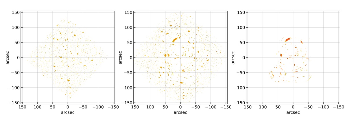
As the characteristic image formation takes place when the source is lying near the caustic, the corresponding magnification is higher. Hence, in such a large source population, we use different magnification cuts to remove undesirable sources. Removal of these sources allows us to easily identify the characteristic image formations near point singularities. An example of such a magnification cut is shown in Figure 1. The left panel represents the unlensed HUDF with all the sources. The middle panel shows the corresponding lensed counterpart with all the sources. Here A370 has been used as the lens and the centers of both A370 and HUDF are aligned with each other without any arbitrary rotation of the lens, i.e., the zeroth realization. As expected the area covered by all the sources in the image plane has been increased after lensing and only the central region shows the strong lensing properties. The right panel represents the same lensed counterpart of left panel but only with the sources that are magnified such that . As mentioned above, doing so removes a significant fraction of sources and allow us to easily see only the highly magnified sources. In actual observation, the availability of spectroscopic information can be used to distinguish different counterparts of the lensed source and identify the possible characteristic image formation. However, as we are only looking at the image formations in our current work, applying different magnification cuts is the only (practical) way to identify the characteristic image formations.
Once we identify and locate image formations, we find out the corresponding source redshift. After finding the source redshift, we replot the lens and source plane only for that particular source along with the critical curves and caustics. As we know the caustic evolution near point singularities, by doing this, we can confirm whether the image formation is due to a point singularity or not. We would like to point out that we have used the second step to eliminate some image formations that are chosen from visual inspection.
5.2 Exotic Image Formation: Purse
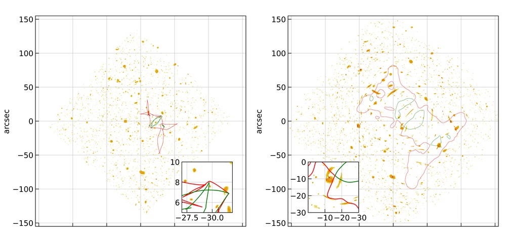
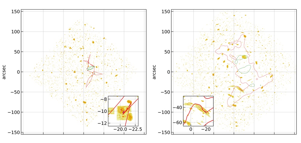
One example of the above-mentioned scheme is shown in Figure 2 for an image formation near purse singularity. Here, the HUDF is lensed due to A370. In this particular case, the center of the HUDF and A370 are not aligned with each other and the lens is rotated by an arbitrary angle. In the top row of Figure 2, the left and right panels represent the unlensed and lensed HUDF images with all of the sources (with ) from N20. The red and green lines represent the caustics and critical curves in the left and right panel, respectively for a source at redshift () 3.7 which is the redshift of the source that is giving rise to the characteristic image formation. Again as expected, only the sources near the center of the cluster lens are strongly lensed and others are only weakly lensed and that the lensed HUDF patch covers more area than the unlensed HUDF patch.
In Figure 2, one can see that the exotic image formation near purse singularity has a small overlap with a different source. Significant overlap with other sources can lead to additional challenges in the identification of exotic image formation near point singularities. As mentioned above, one can deal with such difficulties if spectroscopic observations of the sources are available. In our current work, we apply magnification cuts on the sources in order to remove the unrequired sources and possible overlap with exotic image formation. The bottom row in Figure 2, represents the top row with a threshold magnification () of 30. One can see that this removes a large fraction of the sources along with the overlapping source and one can clearly see the exotic image formation (ring like structure) near purse singularity. The inset plots show the corresponding zoomed regions near the source and characteristic image formation in the source and lens planes.
The other important feature observed in this particular realization is the fact that only a part of the source (which is inside the both radial and tangential caustics) is responsible for the exotic image formation which leads to the observations of merging images in these exotic image formations. One would have observed four separate images if the complete source was within the caustics. The current image formation shows one possible variation of the purse image formation. So far (best to our knowledge), only one image formation near purse is observed (Limousin et al., 2008; Orban de Xivry & Marshall, 2009) in cluster lens Abell 1703.
5.3 Exotic Image Formation: Swallowtail
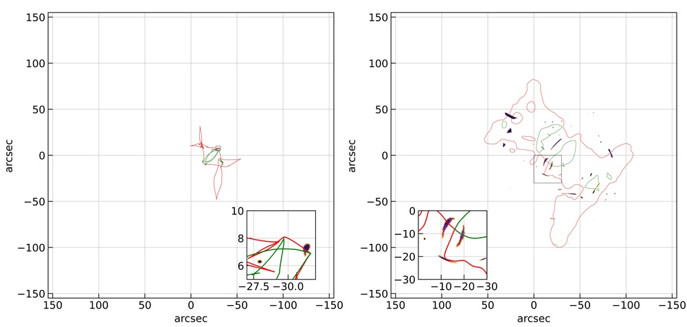
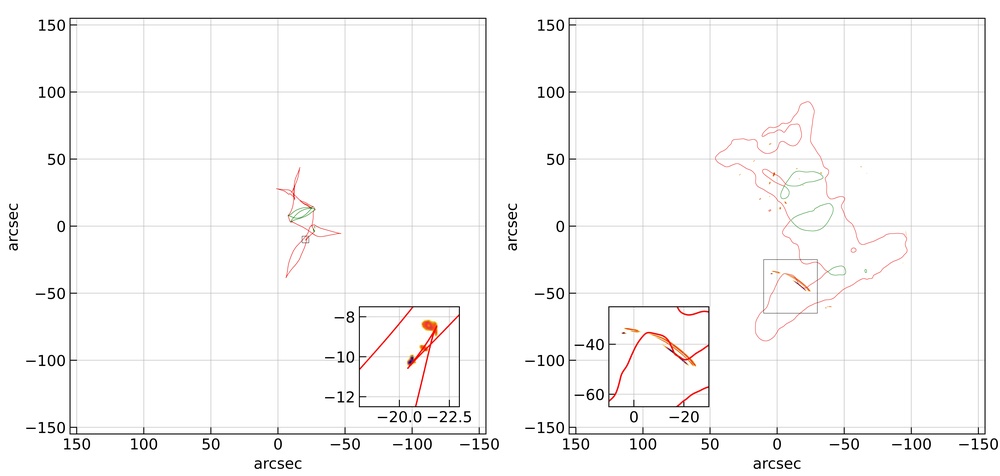
Another example of exotic image formation near swallowtail singularity is shown in Figure 3. Here again, the cluster lens is A370. However, the lensing realization is different from Figure 2 meaning that the lens alignment and rotation angle is different. Again, the top row in Figure 3 shows the unlensed and lensed HUDF in the left and right panel, respectively, with all the sources having source redshift . The red and green lines represent the caustics and critical curves in the left and right panels, respectively, for a source redshift () of 2.5. The bottom row is the same as the top row but with a threshold magnification () of 30. As the sources are extended galaxy sources, one can see that only a handful of source are left with a magnification . The inset plots show the corresponding zoomed regions near the source and characteristic image formation in the source and lens planes.
As we know from MB20, the characteristic image formation for a swallowtail singularity is an arc made of four images which we also observe in the 3. However, in Figure 3, instead of having an overlap of multiple sources (like Figure 2), we observe three different sources lying near the swallowtail singularity and giving rise to corresponding image formation. The galaxy source in the middle of the inset plot is at redshift 2.5, and the bottom (top) source lies at a redshift 2.62 (2.86). Such image formations where several sources are lying near the point singularity can be observed for both swallowtail and purse. However, as the probability of observing two sources near each other in the sky as well as in redshift is small, one does not expect to such juxtaposition very often. Observations have led us to the detection of a handful of cases with image formation near swallowtail singularity in both galaxy (e.g., Suyu & Halkola, 2010) and cluster scale lenses (e.g., Abdelsalam et al., 1998).
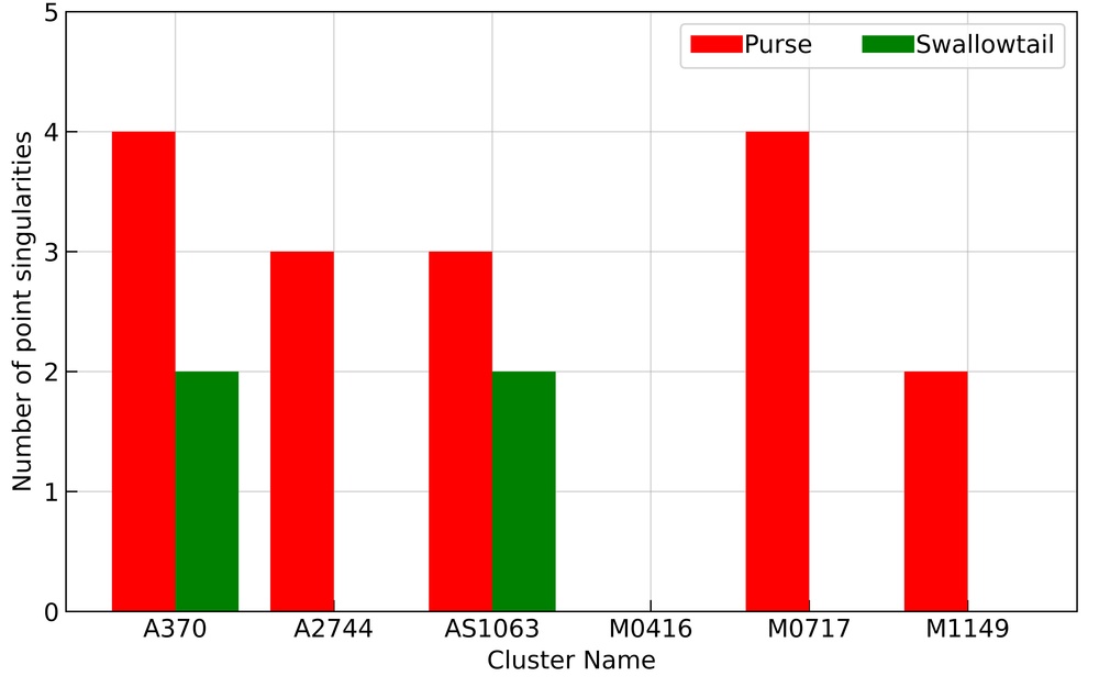
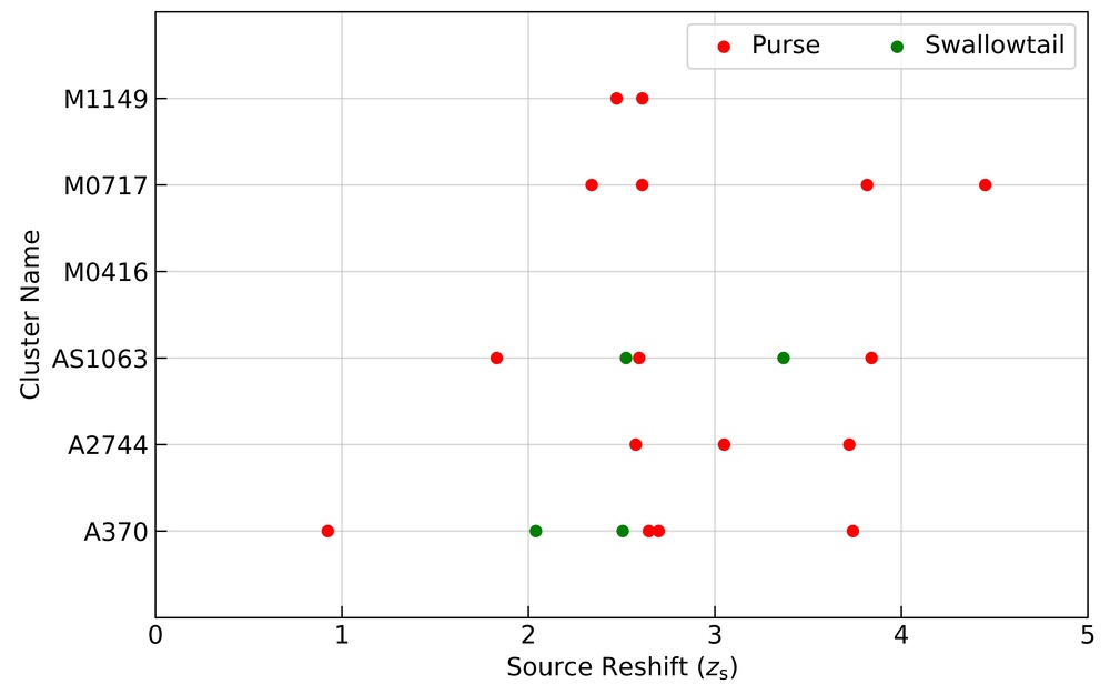
In Figures 2 and 3, we only showed one example of exotic image formation near both purse and swallowtail singularities with A370 as the cluster lens. However, there are other realizations where we have identified the image formation near these point singularities. All these image formations (including from Figure 2 and 3) are available as supplementary material. In Figure 4, we show the number and redshift distribution of all exotic image formations identified in the HFF cluster lenses. The left panel represents the number distribution of the exotic image formations in the HFF clusters, whereas the right panel represents the corresponding redshift distribution. In the eleven realizations corresponding to the A370, we identified a total of four image formations near the purse and three near the swallowtail singularity. On the other hand, we did not observe any exotic image formation in M0416 realizations. This again backs up the earlier result of paper-ii that A370 (M0416) is the most (least) efficient in producing image formation near point singularities in all of the HFF clusters considering the best-fit grale lens mass models.
From the redshift distribution of exotic image formations in the right panel, one can see that most of the images are identified in the redshift range [1, 4]. Such a result is expected as at the lower redshifts, the strong lensing region in the cluster is small, and at higher redshifts, the source density decreases. However, we again remind the reader that here we are only considering half of the sources from HUDF. Increasing the number of sources increases the probability of observing such image formation at both low and high redshift.
5.4 Time Delay Analysis
Various point singularities mark the points in the source plane where cusp are created or destroyed or exchanged between radial and tangential caustic. Hence, the characteristic image formations are only observed if the source lies near the caustics in the source plane. This implies that the time delay between various images, which are part of the characteristic image formation, should be smaller than a typical strong lensing scenario where the source lies sufficiently far away from point caustics.
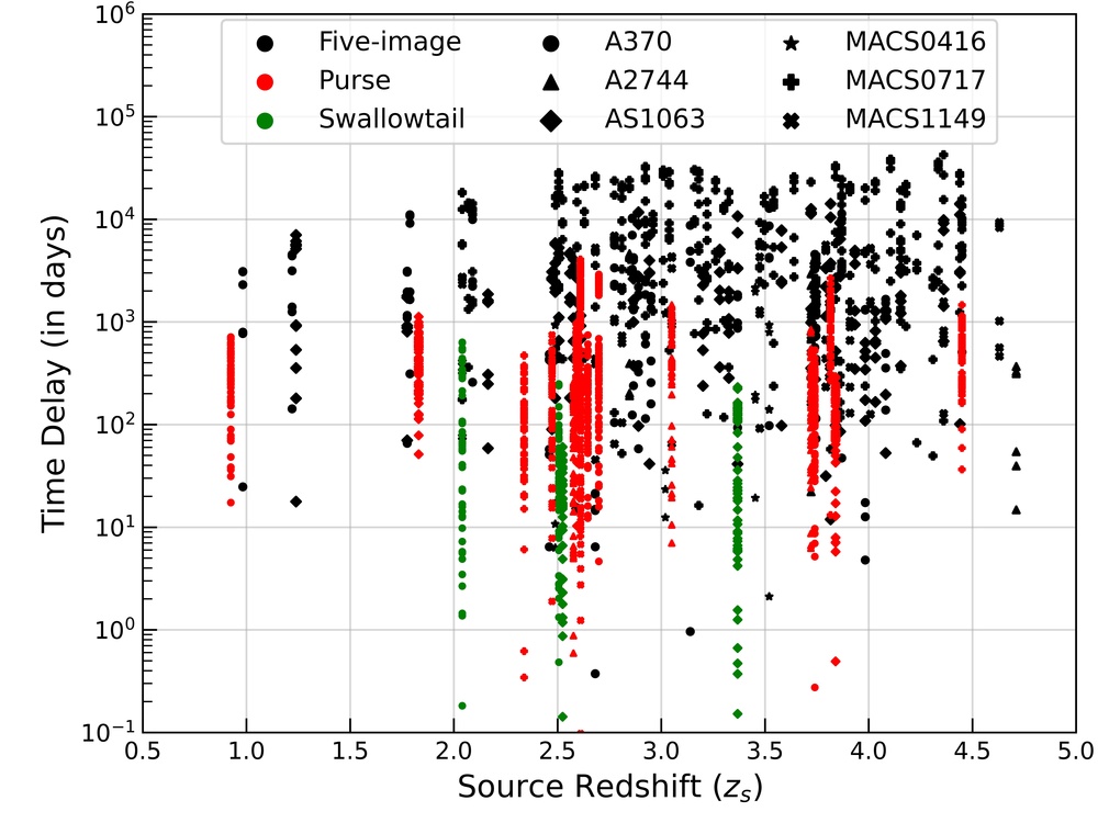
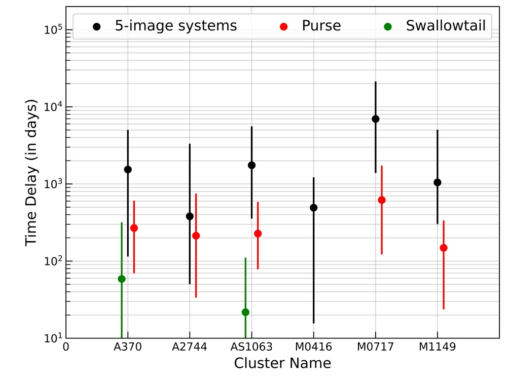
We calculate the time delay between different image pairs for each identified exotic image formation in all realization. Figure 5, represents the time delay values in five-image geometry and in purse and swallowtail image configurations. The left panel is a combined plot of the time delay for five-image (black points), purse (red points) and swallowtail (green points) geometry found in all realizations for all of the HFF clusters. Here we removed the global minima image from all the systems. Doing so leads to a total of six pairs of time-delays for one five-image system. As the number of image formations near purse and swallowtail is very small compared to the number of typical five-image cases, we draw a circle around the identified purse and swallowtail image formation and choose ten different random source position and calculate the corresponding time delays. Doing so allow us to estimate the possible variation in the time delay associated with one particular system.
One can see that the a typical five image geometry gives time delay values in range days. On the other hand, image formations near purse and swallowtail (except for a few geometries) always remain less than 1000 days which is smaller than the typical five-image geometry time delay. This is evident from the right panel of Figure 5, where we show the median time delay values for each HFF cluster separately. Again, one can see that the median value for five-image geometry for each HFF is nearly an order of magnitude larger than the purse and swallowtail geometry. The error bars around these median points cover the range between and percentile.
From left and right panels, one can also notice that, in general, the swallowtail geometry leads to smaller time delays compared to the purse geometry. The time-delays corresponding to the pyramid singularity would have been even smaller than the swallowtail but the grale best-fit mass models for HFF cluster only give one pyramid point (in MACS1149) leading to a negligible cross-section. Hence, we do not study the image formation or time-delay analysis for the pyramid singularities in our current work. However, the same is not true for the parametric mass models. As we have see in paper-i, the number of pyramid singularities are significantly larger compared to the non-parametric mass models encouraging us to include pyramid in our future analysis.
6 Conclusions
In our current work, we have investigated lensed HUDF templates for exotic image formations near point singularities. The best-fit grale mass models of the HFF cluster are chosen as the lens mass models as they provide the lowest cross-section for the point singularities (see paper-i and paper-ii). We constructed eleven realizations of the lensed HUDF for every HFF cluster with different random orientations. The alignment of the HFF clusters and the HUDF is chosen such that the critical lines for a source at redshift ten are always confined within the HUDF region. As the HUDF contains galaxy sources at various redshifts, the corresponding source cutouts (only for 5271 sources from N20) are used for lensing in current work. At present, we do not have an automated algorithm to locate these image formations. Hence, we visually inspected each of the realizations to identify the exotic image formation. Out of 66 realizations, in 4 (16) realizations, we identified image formations near the swallowtail (purse) singularity. In this work, we do not look for the image formation near a pyramid singularity as the best-fit grale mass models for the HFF clusters only give one pyramid singularity in MACS1149.
It is noteworthy that the number of realizations of purse singularity is much higher than swallow tail. This suggests that purse may be more common than swallow tail in deep observations. This possibility needs to be explored with a larger set of cluster lenses.
Apart from image formation near point singularities, we also study the time delay between multiple images in these exotic image formations. We find that typical time delay in swallowtail and purse image formations are an order of magnitude smaller than a typical five image geometry in the HFF clusters (after removing the global minima). Such a difference can be very helpful in time-delay cosmography to constrain the Hubble constant.
The key takeaway points of our current analysis is that the number of image formation near point singularities are not negligible whether we estimate the number using source galaxy population or by using the simulated patches of the sky. The corresponding time-delay values are significantly smaller than typical image formation in the cluster lenses.
Now that we have shown that the number of such systems is not small, the following questions need to be addressed: (i) What is the effect of the line-of-sight (off-plane) structures on the number of point singularities for a given lens? (ii) How to identify these image formations (including pyramids) in the all-sky surveys? In order to account for the line-of-sight structure (if far away from the main lens), one needs to use double-plane (or multi-plane) lensing. As discussed in the previous work (Levine & Petters, 1993; Kayser & Schramm, 1993), new type of singularities may also arise in the double plane lensing which can further complicate the analysis. Although the current analysis allows us to see variations in the image formations near point singularities, it is not complete. The best-fit grale mass models underestimate the small scale structures. Hence, the above identified image formations only cover a small fraction of possible variations in exotic image formation. One can use both parametric and non-parametric mass models to construct a catalog of possible image formations near point singularity. Such a catalog can be helpful in automated searches in all-sky surveys (e.g., Lanusse et al., 2018; Avestruz et al., 2019; Davies et al., 2019). These problems are subjects of our future work, and the results will be presented in forthcoming publications.
7 Acknowledgements
AKM would like to thank Council of Scientific Industrial Research (CSIR) for financial support through research fellowship No. 524007. Authors would like to thank Liliya Williams for providing lens mass models for the HFF clusters. JSB would like to thank Yannick Mellier for suggesting the use of deep fields as sample source population. This research has made use of NASA’s Astrophysics Data System Bibliographic Service. We acknowledge the HPC@IISERM, used for some of the computations presented here.
8 Data Availability
The high resolution HFF cluster mass models corresponding to the Williams group are available from the modelers upon request.
References
- Abdelsalam et al. (1998) Abdelsalam H. M., Saha P., Williams L. L. R., 1998, MNRAS, 294, 734
- Akeson et al. (2019) Akeson R., et al., 2019, arXiv e-prints, p. arXiv:1902.05569
- Andrade et al. (2019) Andrade K. E., Minor Q., Nierenberg A., Kaplinghat M., 2019, MNRAS, 487, 1905
- Andrade et al. (2020) Andrade K. E., Fuson J., Gad-Nasr S., Kong D., Minor Q., Roberts M. G., Kaplinghat M., 2020, arXiv e-prints, p. arXiv:2012.06611
- Annunziatella et al. (2017) Annunziatella M., et al., 2017, ApJ, 851, 81
- Atek et al. (2018) Atek H., Richard J., Kneib J.-P., Schaerer D., 2018, MNRAS, 479, 5184
- Avestruz et al. (2019) Avestruz C., Li N., Zhu H., Lightman M., Collett T. E., Luo W., 2019, ApJ, 877, 58
- Beckwith et al. (2006) Beckwith S. V. W., et al., 2006, AJ, 132, 1729
- Bertin & Arnouts (1996) Bertin E., Arnouts S., 1996, A&AS, 117, 393
- Blandford & Narayan (1992) Blandford R. D., Narayan R., 1992, ARA&A, 30, 311
- Bouwens et al. (2015) Bouwens R. J., et al., 2015, ApJ, 803, 34
- Brainerd (2010) Brainerd T. G., 2010, ApJ, 713, 603
- Coe et al. (2013) Coe D., et al., 2013, ApJ, 762, 32
- Collett (2015) Collett T. E., 2015, ApJ, 811, 20
- Cowley et al. (2018) Cowley W. I., Baugh C. M., Cole S., Frenk C. S., Lacey C. G., 2018, MNRAS, 474, 2352
- Davies et al. (2019) Davies A., Serjeant S., Bromley J. M., 2019, MNRAS, 487, 5263
- Driver & Robotham (2010) Driver S. P., Robotham A. S. G., 2010, MNRAS, 407, 2131
- Finkelstein et al. (2015) Finkelstein S. L., et al., 2015, ApJ, 810, 71
- Gardner et al. (2006) Gardner J. P., et al., 2006, Space Sci. Rev., 123, 485
- Giavalisco et al. (2004) Giavalisco M., et al., 2004, ApJ, 600, L93
- Harvey et al. (2016) Harvey D., Kneib J. P., Jauzac M., 2016, MNRAS, 458, 660
- Irwin et al. (2007) Irwin J., Shmakova M., Anderson J., 2007, ApJ, 671, 1182
- Ivezić et al. (2019) Ivezić Ž., et al., 2019, ApJ, 873, 111
- Jauzac et al. (2014) Jauzac M., et al., 2014, MNRAS, 443, 1549
- Jauzac et al. (2016) Jauzac M., et al., 2016, MNRAS, 463, 3876
- Johnson et al. (2014) Johnson T. L., Sharon K., Bayliss M. B., Gladders M. D., Coe D., Ebeling H., 2014, ApJ, 797, 48
- Joseph et al. (2019) Joseph R., Courbin F., Starck J. L., Birrer S., 2019, A&A, 623, A14
- Kayser & Schramm (1993) Kayser R., Schramm T., 1993, A&A, 278, L13
- Kelly et al. (2015) Kelly P. L., et al., 2015, Science, 347, 1123
- Kelly et al. (2018) Kelly P. L., et al., 2018, Nature Astronomy, 2, 334
- Kneib & Natarajan (2011) Kneib J.-P., Natarajan P., 2011, A&ARv, 19, 47
- Lanusse et al. (2018) Lanusse F., Ma Q., Li N., Collett T. E., Li C.-L., Ravanbakhsh S., Mandelbaum R., Póczos B., 2018, MNRAS, 473, 3895
- Laureijs (2009) Laureijs R., 2009, arXiv e-prints, p. arXiv:0912.0914
- Levine & Petters (1993) Levine H. I., Petters A. O., 1993, A&A, 272, L17
- Li et al. (2016) Li N., Gladders M. D., Rangel E. M., Florian M. K., Bleem L. E., Heitmann K., Habib S., Fasel P., 2016, ApJ, 828, 54
- Liesenborgs et al. (2020) Liesenborgs J., Williams L. L. R., Wagner J., De Rijcke S., 2020, MNRAS, 494, 3253
- Limousin et al. (2008) Limousin M., et al., 2008, A&A, 489, 23
- Lotz et al. (2017) Lotz J. M., et al., 2017, ApJ, 837, 97
- McLeod et al. (2015) McLeod D. J., McLure R. J., Dunlop J. S., Robertson B. E., Ellis R. S., Targett T. A., 2015, MNRAS, 450, 3032
- Meena & Bagla (2020) Meena A. K., Bagla J. S., 2020, MNRAS, 492, 3294
- Meena & Bagla (2021) Meena A. K., Bagla J. S., 2021, MNRAS, 503, 2097
- Meena et al. (2021) Meena A. K., Ghosh A., Bagla J. S., Williams L. L. R., 2021, arXiv e-prints, p. arXiv:2103.13617
- Menci et al. (2017) Menci N., Merle A., Totzauer M., Schneider A., Grazian A., Castellano M., Sanchez N. G., 2017, ApJ, 836, 61
- Meneghetti et al. (2010) Meneghetti M., Rasia E., Merten J., Bellagamba F., Ettori S., Mazzotta P., Dolag K., Marri S., 2010, A&A, 514, A93
- Meneghetti et al. (2017) Meneghetti M., et al., 2017, MNRAS, 472, 3177
- Mohammed et al. (2016) Mohammed I., Saha P., Williams L. L. R., Liesenborgs J., Sebesta K., 2016, MNRAS, 459, 1698
- Montes & Trujillo (2018) Montes M., Trujillo I., 2018, MNRAS, 474, 917
- Morishita et al. (2017) Morishita T., Abramson L. E., Treu T., Schmidt K. B., Vulcani B., Wang X., 2017, ApJ, 846, 139
- Moster et al. (2011) Moster B. P., Somerville R. S., Newman J. A., Rix H.-W., 2011, ApJ, 731, 113
- Nolan et al. (2020) Nolan L., Mechtley M., Windhorst R., Knierman K., Ashcraft T., Cohen S., Tompkins S., Will L., 2020, arXiv e-prints, p. arXiv:2012.09994
- Oesch et al. (2007) Oesch P. A., et al., 2007, ApJ, 671, 1212
- Oesch et al. (2013) Oesch P. A., et al., 2013, ApJ, 773, 75
- Oguri (2010) Oguri M., 2010, PASJ, 62, 1017
- Oguri & Marshall (2010) Oguri M., Marshall P. J., 2010, MNRAS, 405, 2579
- Ono et al. (2013) Ono Y., et al., 2013, ApJ, 777, 155
- Orban de Xivry & Marshall (2009) Orban de Xivry G., Marshall P., 2009, MNRAS, 399, 2
- Parsa et al. (2016) Parsa S., Dunlop J. S., McLure R. J., Mortlock A., 2016, MNRAS, 456, 3194
- Plazas et al. (2019) Plazas A. A., Meneghetti M., Maturi M., Rhodes J., 2019, MNRAS, 482, 2823
- Priewe et al. (2017) Priewe J., Williams L. L. R., Liesenborgs J., Coe D., Rodney S. A., 2017, MNRAS, 465, 1030
- Rafelski et al. (2015) Rafelski M., et al., 2015, AJ, 150, 31
- Raney et al. (2020) Raney C. A., Keeton C. R., Brennan S., Fan H., 2020, MNRAS, 494, 4771
- Rix et al. (2004) Rix H.-W., et al., 2004, ApJS, 152, 163
- Rowe et al. (2013) Rowe B., Bacon D., Massey R., Heymans C., Häußler B., Taylor A., Rhodes J., Mellier Y., 2013, MNRAS, 435, 822
- Schneider et al. (1992) Schneider P., Ehlers J., Falco E. E., 1992, Gravitational Lenses, doi:10.1007/978-3-662-03758-4.
- Scoville et al. (2007) Scoville N., et al., 2007, ApJS, 172, 1
- Sendra et al. (2014) Sendra I., Diego J. M., Broadhurst T., Lazkoz R., 2014, MNRAS, 437, 2642
- Strait et al. (2018) Strait V., et al., 2018, ApJ, 868, 129
- Suyu & Halkola (2010) Suyu S. H., Halkola A., 2010, A&A, 524, A94
- Thompson et al. (2006) Thompson R. I., Eisenstein D., Fan X., Dickinson M., Illingworth G., Kennicutt Robert C. J., 2006, ApJ, 647, 787
- Treu & Marshall (2016) Treu T., Marshall P. J., 2016, A&ARv, 24, 11
- Williams et al. (2018) Williams L. L. R., Sebesta K., Liesenborgs J., 2018, MNRAS, 480, 3140
- Yang et al. (2020) Yang L., Birrer S., Treu T., 2020, MNRAS, 496, 2648
- Zitrin & Broadhurst (2009) Zitrin A., Broadhurst T., 2009, ApJ, 703, L132
- Zwicky (1937) Zwicky F., 1937, Physical Review, 51, 290