Expectation Maximization Aided Modified Weighted Sequential Energy Detector for Distributed Cooperative Spectrum Sensing
Abstract
Energy detector (ED) is a popular choice for distributed cooperative spectrum sensing because it does not need to be cognizant of the primary user (PU) signal characteristics. However, the conventional ED-based sensing usually requires large number of observed samples per energy statistic, particularly at low signal-to-noise ratios (SNRs), for improved detection capability. This is due to the fact that it uses the energy only from the present sensing interval for the PU detection. Previous studies have shown that even with fewer observed samples per energy statistics, improved detection capabilities can be achieved by aggregating both present and past ED samples in a test statistic. Thus, a weighted sequential energy detector (WSED) has been proposed, but it is based on aggregating all the collected ED samples over an observation window. For a highly dynamic PU over the consecutive sensing intervals, that involves also combining the outdated samples in the test statistic that do not correspond to the present state of the PU. In this paper, we propose a modified WSED (mWSED) that uses the primary user states information over the window to aggregate only the highly correlated ED samples in its test statistic. In practice, since the PU states are a priori unknown, we also develop a joint expectation-maximization and Viterbi (EM-Viterbi) algorithm based scheme to iteratively estimate the states by using the ED samples collected over the window. The estimated states are then used in mWSED to compute its test statistics, and the algorithm is referred to here as the EM-mWSED algorithm. Simulation results show that EM-mWSED outperforms other schemes and its performance improves by increasing the average number of neighbors per SU in the network, and by increasing the SNR or the number of samples per energy statistic.
Index Terms:
Cognitive radios, dynamic primary user, distributed cooperative spectrum sensing, expectation-maximization, energy detector, modified weighted sequential energy detector, Viterbi.I Introduction
A cognitive radio system is an intelligent wireless communication system that learns from its surrounding radio environment and adapts its operating parameters (e.g., carrier frequency, transmit power, and digital modulation scheme) in real-time to the spatiotemporal variations of the RF spectrum. The primary objective of the cognitive scheme is to enable the unlicensed (secondary) users to opportunistically utilize the spectrum owned by the licensed (primary) users, where the reconfigurability of the radio is accomplished using software-defined radio based platforms [1, 2, 3]. However, the opportunistic access of the wireless spectrum entails using the spectrum sensing algorithm at the secondary users (SUs) to detect the presence or absence of the primary user (PU) in the channel. For the detection of PU, several sensing algorithms have been presented over the past years including the energy detector (ED) [4], coherent ED [5], matched filter detector [6], cyclostationary feature detector [7, 8], information theoretic criterion based detector [9], and eigen-values based detectors [10, 11]. These detectors make different trade-offs between the spectrum sensing delay, computational complexity, and the amount of PU’s signal information needed for sensing. Among these detectors, ED stands out as a preferred choice because of its low computational complexity, ease of implementation, and due to the reason that it does not require any prior knowledge about the PU signal. As such, ED-based spectrum sensing has been exploited widely in the literature, e.g., [12, 13, 14, 15], including the present paper.
Spectrum sensing (or PU detection) can be done by the SUs either by using a non-cooperative scheme or a cooperative scheme. In a non-cooperative scheme, each SU performs PU detection individually without any direct communication with the other SUs or a fusion center (FC) [13, 11]. In contrast, in cooperative spectrum sensing, a group of SUs communicate with each other or with an FC to collaboratively perform the PU detection [15, 16, 17]. Consequently, in comparison, the cooperative sensing approach is resilient to the deep fading and shadowing at an SU level, aids in eliminating the hidden terminal problem, reduces the sensing duration per SU, and demonstrates a better detection performance across the SUs network[18, 19].
Cooperative spectrum sensing schemes can be further categorized into either a centralized scheme or a distributed scheme. In a centralized scheme, a fusion center collects the sensing information from the SUs, detects the unused band, and broadcasts the decision to the SUs [20, 16, 15, 21]. However, the centralized approach is not scalable to large networks as the available communication resources are usually limited at the FC. Furthermore, an FC involvement defines a single point of failure for the centralized network. In comparison, in a distributed scheme, the SUs share their sensing statistics with their neighboring users followed by using a consensus protocol to collaboratively decide on the presence or absence of PU in the channel [22, 23]. This approach not only eliminates the single point of failure from the network, but it is also scalable as the communication resources need to be shared only among the neighbors.
The distributed cooperative spectrum sensing (DCSS) scheme usually has three critical phases, namely the sensing phase, the consensus phase, and the channel use phase. In the sensing phase, a group of SUs observes the PU channel for a certain time duration to collect a sufficient number of samples for computing the summary statistics (e.g., energy statistics [24, 13]). Next, in the consensus phase, the SUs share their summary statistics with their neighbors, and use an average consensus protocol [25, 26] to iteratively compute a weighted average of the globally shared values across the network. Upon consensus in such an approach, the final value is compared against a threshold at each SU to locally detect the presence or absence of the PU in the channel. Finally, in the channel use phase, the detection outcome is used to decide on the opportunistic use of the PU channel before restarting the cycle. This DCSS scheme was proposed in [22] wherein the authors analyzed its convergence speed as well as the detection performance for varying false alarm rates. In [27, 28], DCSS was extended to protect against the eavesdropper attack by encrypting the summary statistics shared between the SUs, whereas in [17, 29], the authors considered the scenarios in which some malicious SUs (aka Byzantines) may share falsified data with the neighbors and thus proposed algorithms to mitigate the Byzantine attacks on the network.
The above-mentioned DCSS algorithms use the conventional approach in which each SU uses energy statistic only from the current sensing interval to make the PU detection. This usually requires a large number of samples per energy statistic, specially for lower SNRs, in order to achieve improved PU detection. As a result, the sensing duration increases which in turn increases the power consumption per SU as well as reduces the network throughput [30]. However, it has been shown that aggregating present and past ED samples at each SU, for lower SNRs, can result in an improved detection performance, even with using a fewer samples per energy statistics [14, 12, 16, 15]. As such, in [15, 16], a dynamic PU is modeled using a two-state Markov chain model and a weighted sequential energy detector (WSED) is proposed in which all the present and past ED samples over an observation window111An observation window is defined as a vector of length containing all the ED statistics from the past sensing periods as well as the ED statistic from the present sensing period. are aggregated to achieve improved detection capability. However, [15, 16] assume a centralized scheme for cooperative spectrum sensing which as discussed before is not a scalable approach. Using the average of past ED samples, a non-cooperative improved ED (IED) is also proposed in [14] in which the averaged value compared against the threshold is used to improve the PU detection probability at lower SNRs. Furthermore, a non-cooperative multi-slot ED (mED) is developed in [12] in which the ED samples from multiple sensing slots are compared against the threshold to detect the presence or absence of PU in the channel.
In this paper, we consider a dynamic PU that follows a two-state Markov chain model for switching between the active and idle states [16, 15]. However, for the PU detection, we develop a test statistic for SUs wherein the highly correlated present and past ED samples are aggregated to improve the PU detection at lower SNRs with a few samples per ED. The SUs deploy the DCSS scheme in which the sensed test statistics are shared between the neighboring users to reach a consensus on the observed value across the network. The contributions made in this paper are listed as follows:
-
•
A modified WSED (mWSED) is proposed in which only those past and present ED samples are aggregated in its test statistics that correspond to the PU’s state in the current sensing interval. Thus, in contrast to the detectors presented in [15, 12, 14], mWSED avoids including the outdated ED samples in its test statistics which improves the detection performance of SUs at lower SNRs (see the simulation results provided in Section III-A and Section V). The closed-form equations for the probability of detection and probability of false alarm are also derived for mWSED.
-
•
An underlying assumption in mWSED is that the actual present and past states visited by the PU are a priori known over the observation window. In practice, the states are unknown, and thus we develop a joint expectation-maximization (EM) and Viterbi based algorithm, referred to herein as EM-Viterbi, to estimate them using the ED samples collected over the window. Specifically, the EM algorithm provides an estimate of the model parameters of the joint probability distribution over the observation vector and the state vector. Next, using their estimate, the Viterbi algorithm [31] optimally estimates the latent state vector by the maximization and back tracing operations and using the properties of the two-state Markov chain model. The estimated state vector produced by the EM-Viterbi algorithm is then used in mWSED to aggregate only the highly correlated samples in its test statistic. The resulting algorithm is named here as the EM-mWSED algorithm.
-
•
Simulation results are included that demonstrate the estimation performance of EM-Viterbi and compare its detection performance with that of the EM-mWSED algorithm. Further, the detection performance of EM-mWSED is compared with the performances of other schemes in the literature. The results show that EM-mWSED performs better than the other methods and its detection performance improves by either increasing the average number of connections per SU in the network, or by increasing the SNR or the number of samples per energy statistics.
This paper is outlined as follows. Section II provides a brief review of the energy detection based spectrum sensing. Distributed cooperative spectrum sensing is discussed in Section III, also including a review of WSED and presentation of our proposed mWSED. Next, Section IV delivers an expectation-maximization and Viterbi algorithm based scheme for estimating the PU states over an observation window, including using it for mWSED. Simulation results are presented in Section V. Finally, Section VI summarizes this work.
II Energy Detector Based Spectrum Sensing
We consider a distributed spectrum sensing system in which a network of SUs are spatially distributed and cooperating with each other to detect the PU in the channel. As discussed in the previous section, we assume that the SUs deploy an energy based statistic to sense the channel. Thus, the energy computed by an -th SU under the null hypothesis () and the alternate hypothesis () can be written as follows.
| (1) |
in which is the total number of samples collected over the sensing interval, is the channel gain for SU , represents the PU signal at time index , and finally, denotes the noise in the sensing interval which is assumed to be normally distributed with zero mean and variance . The signal to noise ratio (SNR) at the SU is defined by which is times the SNR at the output of the energy detector. The ED statistics in (1) follow a central chi-squared distribution with degrees of freedom under , and a non-central chi-squared distribution with degrees of freedom and non-centrality parameter under [32]. However, for the case of low SNR, we usually need a sufficient large number of samples () per energy statistics for improved PU detection222This can be observed from Eqn. (II) that for smaller values we need larger values to realize non-overlapping distributions of ED statistics under both hypotheses and thereby achieve improved PU detection. However, note that larger implies larger sensing duration which increases the power consumption per SU as well as reduces the network throughput [30]. In this paper, we show that an improved detection capability can be achieved for lower SNRs and values by averaging the highly correlated present and past ED statistics.. Thus, we can invoke the central limit theorem (CLT) [33] to assume that is Gaussian distributed under the hypothesis with mean and variance , for [12, 14]. These means and variances can be computed as
| (2) |
As such, the probability of false alarm () and probability of detection () can be computed as
| (3) |
where is the threshold for energy detection, and is the complementary cumulative distribution function of Gaussian distribution [33]. Note that for a selected value of false alarm probability, the threshold can be computed from (II) by using the inverse of the function. Furthermore, given , the detection probability can be computed from (II) as well.
III Distributed Cooperative Spectrum Sensing
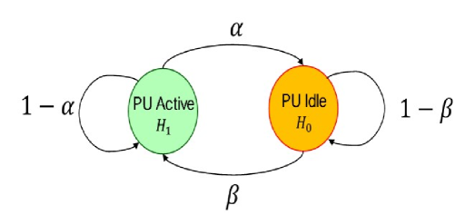
We consider a scenario wherein the PU follows a two-state Markov chain model for switching between the and as shown in Fig. 1 [16, 15]. Specifically, the next state visited by the PU depends only on its immediate previous state. Accordingly, in this figure, the parameter denotes the transition probability of switching to an idle state () given that previously the PU was in the active state (), whereas represents the transition probability of switching to an active state () if previously the PU was in the idle state (). Thus, higher values of and imply a highly dynamic PU, whereas their smaller values represent its slowly time-varying behavior. In the following, we first describe a scalable distributed cooperative spectrum sensing scheme as considered here, followed with a brief review of the WSED algorithm and our modified WSED algorithm.
Consider a network of SUs represented by an undirected graph in which is the set of number of SUs in the network, and represents the set of all possible bidirectional communication links between them. The connectivity of the network in any realization is denoted by which is defined as a ratio of the number of active connections in the network () to the number of all possible connections among the SUs (). We consider a strongly connected network in which the neighboring users that are one hop away from each other share their information to reach a consensus. Therefore, wireless and computing resources such as bandwidth, processing power, and data storage capabilities, need to be only locally managed at the SUs, and scale proportionally to the average number of connections per SU in a network.
A distributed cooperative spectrum sensing algorithm is a scalable and a fully distributed approach which deploys a consensus protocol at an SU. The protocol iteratively updates the sensing information at the user, by using the locally shared information, to reach consensus with the other users in the network. To elaborate, let represents the initial energy statistic for an -th SU, then in iteration of the DCSS algorithm, the SU updates its estimate by using a weighted average method as follows.
| (4) |
in which is the set of neighboring users of the -th SU. The weight can be selected as where and represent the number of neighbors of SU and SU , respectively. This selection of weights results in a doubly-stochastic Metropolis-Hasting weighting matrix which guarantees convergence of the consensus algorithm [26]. Thus, starting with a set of initial values , the algorithm running locally at each SU iteratively updates the values using (4) until it converges to an average of the globally shared values across the network. The average value is defined by . Upon convergence, the decision can be made locally at the -th SU by using the following rule
| (5) |
III-A Simulation Results
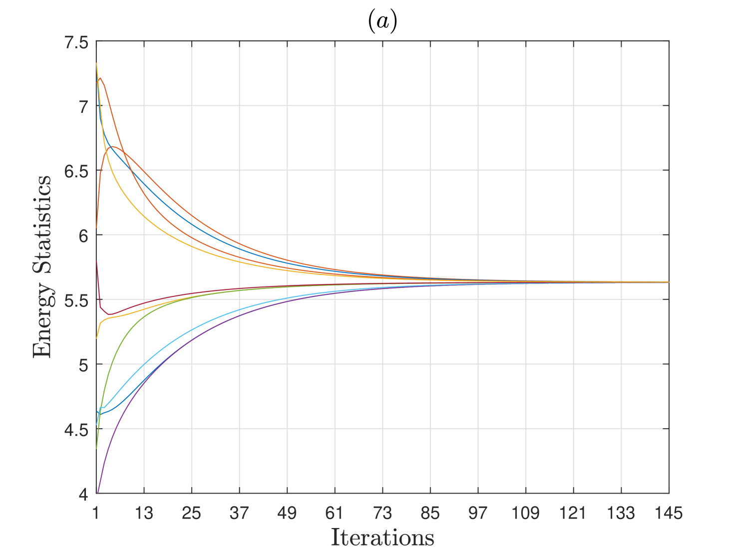
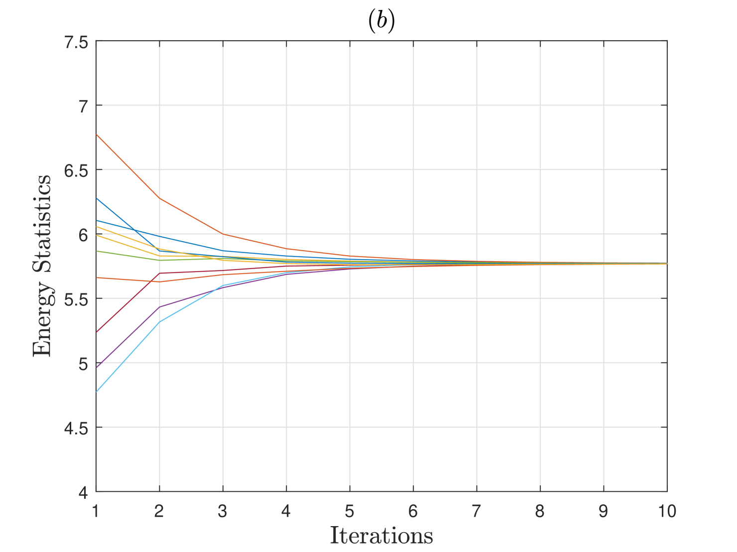
Herein, we analyze the consensus performance of an energy detector (ED) based DCSS scheme when the network of SUs is randomly generated for different number of SUs and with varying connectivity . The primary user follows a two-state Markov chain model for switching states between and over the multiple sensing intervals. Each SU uses samples for computing the energy statistic following (1), and has an SNR dB for the PU channel. In Fig. 2, we demonstrate the convergence performance of the ED-based DCSS algorithm from a single trial for and users when the connectivity is either or . It is observed that when and , the consensus occurs in about iterations, but when the connectivity increases to , it happens in about iterations. Similar observation is made if increases from to SUs for . This is because the average number of connections per SU, i.e., , increases when either or increases, and thus the local averages computed at the SUs in (4) are more accurate and stable resulting in the faster convergence speed.
III-B Weighted Sequential Energy Detector
As proposed in [16, 15], the WSED algorithm computes a weighted sum of all the present and past ED samples over an observation window of length to define a new test statistic, which for the -th SU is given by
| (6) |
where represents the energy statistic of the SU (as in (1)) in the sensing interval , with representing the energy at the present sensing interval. Thus, a total number of present and past ED samples are combined in the WSED statistic. The weights obey and the authors in [16, 15] proposed to use exponential weights () for an improved detection capability. Specifically, the exponential weighting is motivated to reduce the impact of aggregating the outdated past samples in (6) in a highly dynamic scenario. However, a centralized scheme is considered in [16, 15] wherein the SUs forward their statistics in (6) to a fusion center where a decision is made using an OR rule. As discussed before in Section I, the use of a fusion center is a non-scalable approach, so in Section V, we extend WSED to the DCSS scheme of (4) with consensus averaging performed on the ED samples aggregated in (6). Upon consensus, the decision can be made locally at each SU by comparing against a threshold. Finally, as pointed out in [15], the exact closed-form expressions for the probability of detection and the probability of false alarm for WSED are in general intractable to compute analytically, due to the aggregation of ED samples that may correspond to different states of the PU. However, the authors in [15] have derived approximated expressions which are also applicable for the DCSS scheme based WSED.
III-C Modified Weighted Sequential Energy Detector
In this subsection, we present our proposed modified WSED (mWSED). It is based on the motivation that instead of combining all the present and past ED samples over the observation window of length , we combine only those ED samples in the summary statistic upon consensus that belong to the present state of the PU. As such, in mWSED, we begin by assuming that the states visited by the PU over the observation window are known to each SU. Notably, this assumption provides a starting point to derive mWSED, but later on in Section IV we also develop the EM-Viterbi algorithm to compute an estimate of those states at each SU, using the ED samples collected over the window as shown in Fig. 4. Thus, by comparing the present and past states over the observation window, each SU locally combines only those samples that correspond to the state of the PU in the present sensing interval. Therefore, the test statistic computed by mWSED at the -th SU in the present -th sensing interval is defined as
| (7) |
where represents the energy computed by SU in the -th sensing interval and is the PU’s state in that interval with denoting and implying . is a weighted indicator function which outputs a non-zero weight for aggregating if is true, and outputs if is false. Thus, given the state information of PU over the observation window, either is included or excluded from . Notably we assume here that the non-zeros weights are normalized and as such sum to . Finally, the statistic is compared against a threshold at SU to make the PU detection.
Now, let be the number of samples with the non-zero weights in (7), we note that for the assumed perfect PU’s states information in mWSED, the use of uniformly distributed weights (i.e., ) is optimal that do not change the means but aids in reducing the variance of , with increasing , under both and (see Propositions and in [15] for proofs). Furthermore, for this case, the test statistic is central chi-squared distributed with degrees of freedom under , and it is non-central chi-squared distributed with degrees of freedom under and non-centrality parameter . In both these cases, we can define the threshold as to obtain the chi-squared distributions. However, for lower SNR and adequate number of samples per ED, we can use the CLT assumption [33] as before to assume that is Gaussian distributed under with mean and variance for . These means and variances are given by
| (8) |
where and are defined in (II) for . The summation with index is used here to simplify (7) and average the non-zero weighted ED samples where the weight for the -th ED sample is defined by . Since the normalized weights are assumed herein, we can note that the means are not effected by the choice of weights in (III-C) but using aids in reducing the variances of under both and with increasing . Also, note that larger values of can be realized for mWSED by equivalently increasing the length of the observation window () which enables the SUs to combine large number of present and past ED samples. However, this in turn results in improving the detection performance of mWSED as shown later in Section III-D. Finally, using (III-C), the probability of false alarm and probability of detection can be given by
| (9) |
where for a chosen false alarm probability, the threshold can be computed from (III-C) by using the inverse function. Together with the resulting detection probability, the operating point for an SU can be defined as .
III-D Simulation Results
In this subsection, we demonstrate the detection performance of mWSED using the simulation setup of Section III-A. Thus, we assume a randomly generated network of SUs with connectivity , and with samples per ED and SNR dB.
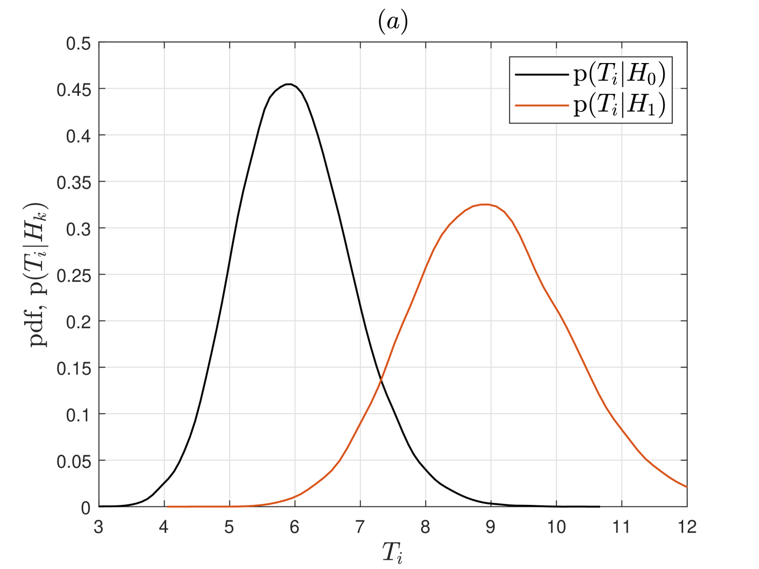
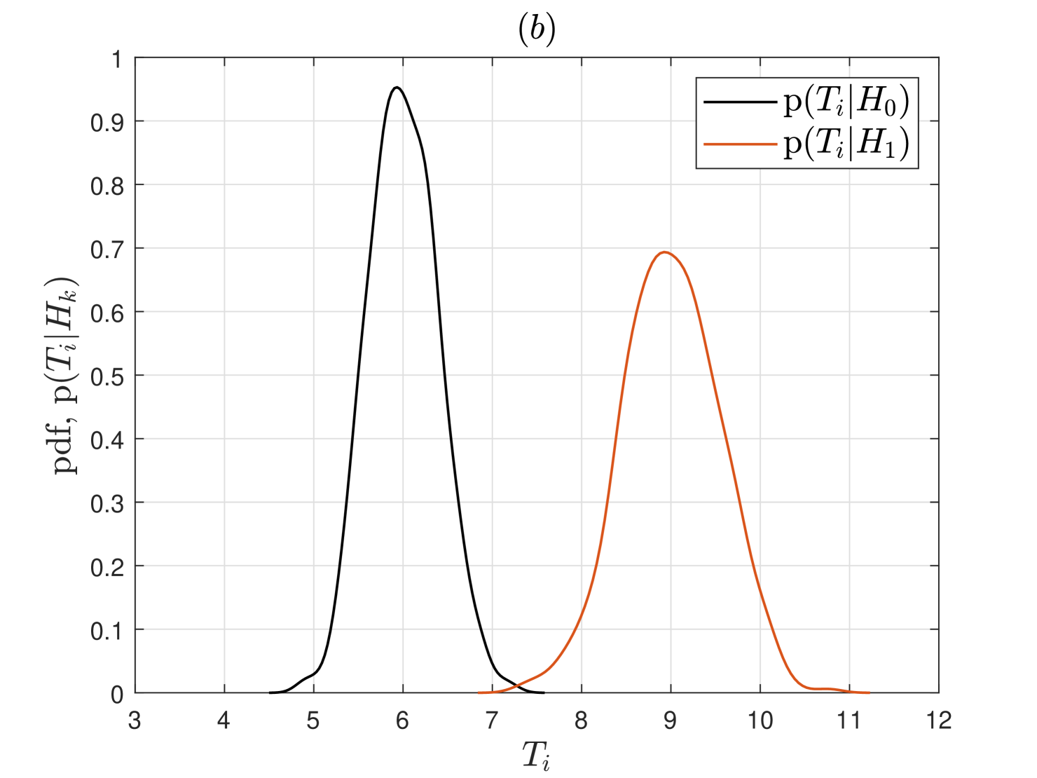
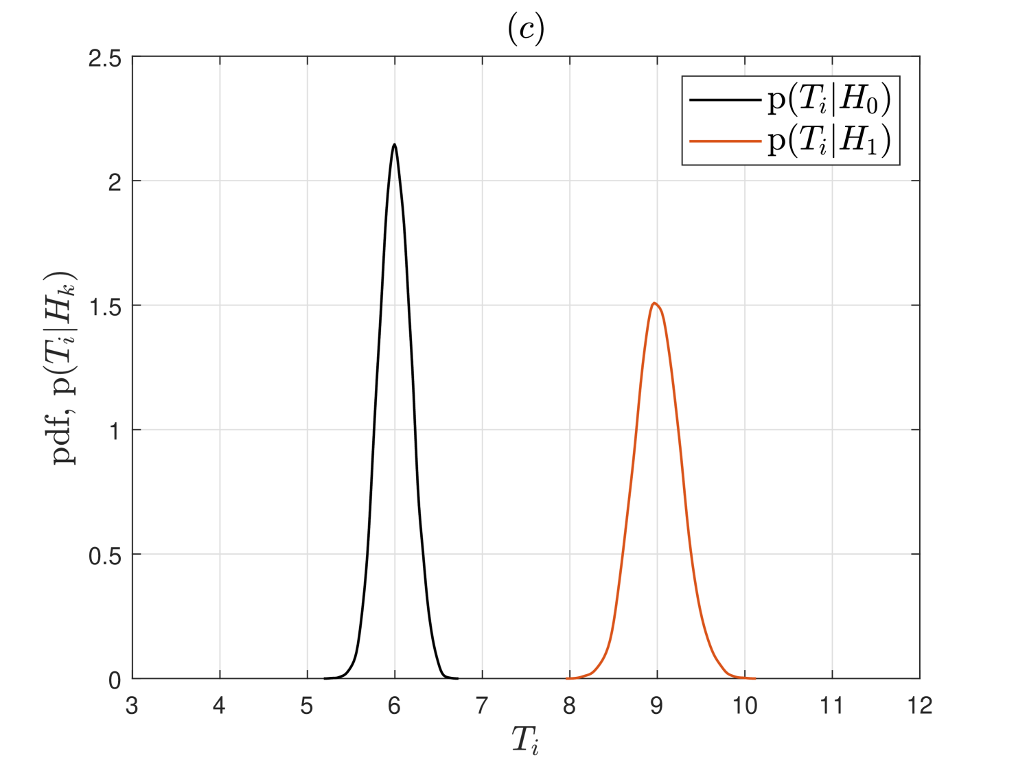
In Fig. 3, we first show the probability density functions (pdfs) of mWSED’s test statistic for SU , under both and , when varying number of ED samples are averaged in . As discussed above for Eqn. (III-C), it is observed in this figure that the means of the test statistic do not change but its variances under both hypotheses decrease with increasing . This elucidates that the detection performance of mWSED will improve when large number of highly correlated ED samples are averaged in its test statistics.
Since a larger value of can be achieved for mWSED by choosing a longer observation window, in Fig. 5, we consider the window length as , for the same network configuration as above, and demonstrate the receiver operating characteristic (ROC) curves for mWSED, WSED, and the conventional ED. The PU follows a two-state Markov model for switching between the active and idle states, and we consider both a slowly time varying PU with and a highly dynamic PU with . We observe that the ED’s performance does not vary with and as it only considers the sample corresponding to the present state of the PU. It is observed that the WSED scheme shows poorer performance for the highly dynamic PU but outperforms ED for a slowly time-varying PU. This is because there are more chances of averaging the outdated samples in WSED in the former case than in the latter one. In contrast, since our mWSED method uses the PU states information to aggregate only the highly correlated ED samples in its test statistics, it outperforms both WSED and ED, and its performance is independent of the time-varying nature of PU.
IV Expectation Maximization Based State Estimation for Dynamic Primary User
The mWSED algorithm described in the previous section assumes that the actual states visited by the PU over the observation window are a priori known to the SUs. In practice, this may not be a valid assumption, and thus in this section we aim to compute an estimate of the states locally at each SU from the samples collected over the observation window.
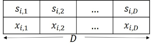
To begin, let an SU collect ED samples over consecutive sensing intervals using (1), denoted by with representing the transpose operation. Using the CLT assumption [33, 17], we assume that follows a Gaussian distribution represented by with mean and variance , and with when the PU is idle, and when the PU is active. These means and variances are defined in (II). Further, if for the -th SU the state of the PU at the sensing interval is denoted by , then for and , the conditional probability distribution of can be written as
| (10) |
where denotes the PU state vector, and is an indicator function which is one if is true, and is zero otherwise [33]. Next, as discussed before and shown in Fig. 1, we assume that the state vector follows a two-state Markov chain model with the transition probabilities and . Thus, the probability distribution of is written as
| (11) |
where considering the steady-state distribution for the Markov process, we assume is Bernoulli distributed with mean .
Now if the model parameters of the above probability distributions are defined by , an optimal scheme for estimating both and for SU involves solving the following optimization problem
| (12) |
where for the sake of simplicity, we assumed a uniform prior distribution on . Note that due to the large dimensionality of the search space, jointly optimizing for and is computationally difficult. Alternatively, we can aim to sequentially optimize for and which involves solving the following two optimization problems:
| (13) |
where (IV) maximizes the likelihood function of . Then using we can solve,
| (14) |
However, note that due to the log-sum in (IV), directly optimizing for the elements of , e.g., using the derivative trick, does not result in the closed-form update equations, whereas using the numerical methods for optimization have the inherent complexity with the tuning of the step-size parameter [34]. Furthermore, the optimization problem in (IV) is still a complex combinatorial search problem where the dimensionality of the search space increases exponentially with . In the following, we develop a joint expectation maximization and Viterbi (EM-Viterbi) algorithm to estimate and in a computationally efficient and optimal way using the closed-form update equations.
IV-A Expectation Maximization Algorithm
An expectation maximization algorithm [35, 36, 37] is an iterative algorithm which can be derived by first selecting a complete data model in order to compute an objective function of the model parameters. Next, given an initial estimate of the parameters, it tends to improve this estimates in each iteration by maximizing the objective function which in turn maximizes the likelihood function[36]. The EM algorithm has been developed for a variety of estimation problems in recent years [38, 39, 36], and in this subsection, we develop it to facilitate joint PU states and the model parameters estimation in order to enable distributed cooperative spectrum sensing using our proposed mWSED scheme.
To begin, let the complete data model for the -th SU be denoted by , and suppose is the -st estimate of the model parameters, then in the -th iteration it computes an expectation step (E-step) and a maximization step (M-step). In the E-step, it computes an expectation of the complete data log-likelihood function as follows
| (15) |
where we note that the expectation is with respect to the posterior distribution on given and an old estimate . In the M-step, it maximizes the objective function in (15) with respect to by solving
| (16) |
in which represents the new estimate of in the -th iteration. The above E-step and M-step are repeated iteratively by replacing the old estimate with the new one until convergence is achieved.
| (17) |
Now using the distributions in (10) and (IV), and the following notation for the expectation operations, i.e., and , for , it can be easily derived that the objective function in (15) can be written as shown in (IV-A). Further, note that and for , where these probability distributions are derived in the Appendix.
In order to compute the M-step in (16), we use the sequential optimization approach [38, 39] for simplicity, i.e., we maximize with respect to each parameter individually by keeping the others fixed to their current estimate. To that end, we use the derivative trick, and thus to maximize with respect to for , we compute its derivative and set it equal to zero as follows.
| (18) |
solving it gives us a new estimate of , in the -th iteration of EM, which is written as333 Note that upon EM’s convergence, we can use (II) and thus divide the ’s estimate obtained from (19) by the number of samples per ED () to estimate the noise power of the PU’s channel (). This noise power estimate can be used to compute the threshold using (II) and (III-C).
| (19) |
for . Now to maximize with respect to , we solve
| (20) |
from which we get the update equation for as
| (21) |
where . Similarly, using the same approach, it can be easily shown that the update equations for the Markov chain transition probabilities and are given by
| (22) | ||||
| (23) |
Thus, all the model parameters are updated iteratively in EM using the closed-form update Eqns. (19), (21), (22), and (23) until convergence is achieved.
Finally, upon the convergence of EM, the state vector for the -th user can be estimated, in a computationally efficient and optimal way, by using the Viterbi algorithm [31]. Thus, at SU , let the EM estimate of the model parameters is denoted by , then the Viterbi algorithm uses it to recursively solve the following optimization problem
| (24) |
for with the initialization . The distributions and are given in (10) and (IV), respectively, and note that they are computed in (24) using only the required parameters estimate from the set . Hence, by keeping track of the maximizing sequence at each time instant in (24) and by finding at time instant , we can back trace the most probable sequence to get .
-
1)
Use the distributed consensus algorithm of (4) to reach consensus
-
6)
Use the Viterbi algorithm in (24) to estimate the PU state vector for SU .
-
7)
Compute the test statistics for mWSED using (7) and compare it against a threshold to make PU detection.
Note that the combination of EM and Viterbi algorithm is named here as the EM-Viterbi algorithm. However, once the state vector of the PU is estimated then we can use it in the mWSED algorithm proposed in Section III-C to combine only the highly correlated ED samples in its test statistic, and the resulting algorithm is referred to here as the EM-mWSED algorithm. Both EM-Viterbi and EM-mWSED are summarized for SU in Algorithm 1.

The computational complexity of EM-mWSED is dominated by the use of the distributed consensus algorithm of (4) in Step . This step has the complexity of per its iteration, where is the cardinality of the set of neighboring users of SU . Furthermore, the forward and backward passes on the observation window in Steps and , to compute the distributions in (VI) and (VI), respectively, as well as the Viterbi algorithm in Step and (24) also dominate the computational complexity. These steps have the complexity of where is the length of the observation window. Thus, the computational complexity of EM-mWSED is where is the number of consensus iterations whereas denotes the number of EM iterations till convergence. The complexity of the energy detector based DCSS is whereas that of the WSED based DCSS is . Thus, the performance improvement of EM-mWSED, as demonstrated in the next section, is at the cost of a slight increase in the computational complexity per a single iteration of the EM algorithm.
V Simulation Results
In this section, we demonstrate the PU detection and states estimation performances of our proposed EM-Viterbi algorithm and the detection performance of our proposed EM-mWSED scheme. For comparison purposes, we compare the performances of these algorithms to the conventional energy detector (ED), the weighted sequential energy detector (WSED) of [16, 15], multi-slot ED (msED) of [12], and the improved ED (IED) of [14] under different scenarios, when these detectors are used with the DCSS scheme and with the consensus happening on the present and past ED samples as proposed herein. As suggested in [16, 15] for WSED, we use a total of past ED samples in its test statistics for a highly dynamic PU, whereas ED uses only the present energy sample in its test statistics. For the msED, we consider only the present and past ED samples for a fair comparison and plot its performance when slots are used in making the PU detection [12]. Notably increasing the number of slots for msED results in a degraded performance for the considered time-varying PU. We consider a network of secondary users randomly generated with a connectivity and the weighting matrix as defined in (4). The average number of connections per SU in the network is given by . The primary user follows a two-state Markov chain model to switch between the active and idle states with the transition probabilities and . The SUs collect samples individually to compute the energy statistic, and the length of the observation window is set as . As described in Algorithm 1, we assume that the SUs reach consensus on all the present and past ED samples over the observation window, which improves the SNR proportionally to and aids in improving the detection and estimation performances. For the initialization of the EM algorithm, we determine the initial estimate of the means and variances by using the K-means clustering algorithm [36] over the window with , whereas the initial estimate of the transition probabilities can be computed by performing a coarse grid search over the likelihood function in (IV) in the interval with a grid resolution of .
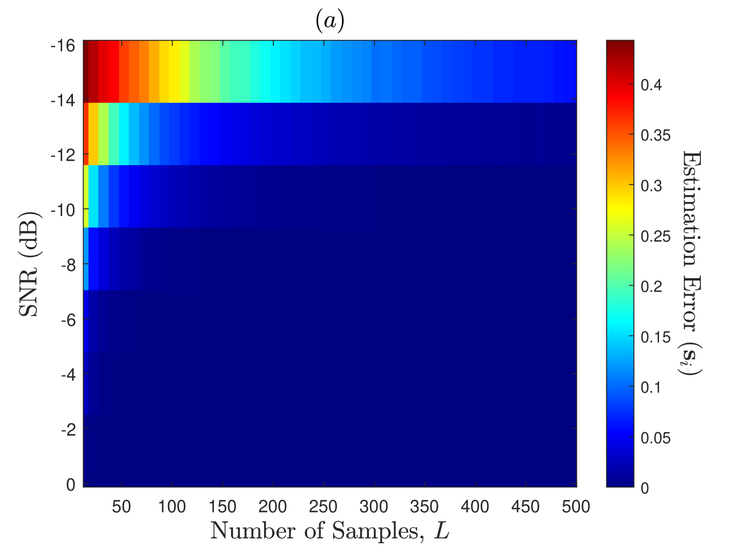
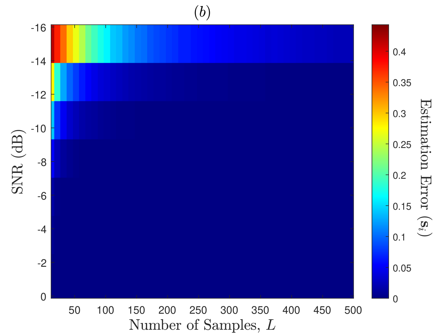
In Fig. 6, we demonstrate the PU’s states estimation performance of the EM-Viterbi algorithm as a function of SNR (dB) and the number of samples per energy statistics (). The states estimation error for SU is defined here as where the expectation is computed over several Monte Carlo trials. Further, we assume that the consensus is reached on the ED samples in Step of Algorithm 1 prior to estimation, and thus the error plots in this figure are observed at all the SUs in the network. We consider here that the secondary users network has , , and users with connectivity . The PU displays a highly dynamic nature with transition probabilities . Firstly, it is observed that for a fewer number of SUs () in the network, the estimation error is higher at the lower SNRs and the lower values, but when the number of SUs in the network increases from to and then to , the estimation error decreases significantly even for the lower SNR and values. This is because the SNR upon consensus in Step 1 of Algorithm 1 improves proportionally to , as each SU exploits about independent ED samples of the PU’s channel. This implies that better performance can be achiever at lower PU’s SNR environments by deploying DCSS-based larger and highly connected networks of SUs, i.e., networks with larger and values., This explains our motivation behind using DCSS scheme prior to the estimation process in Algorithm 1. Secondly, as discussed in Section I, it is observed that the estimation error is higher at lower SNR and values for all the considered cases in Fig. 6. As discussed in Section II, this is because the distribution of the ED samples under the two hypotheses highly overlap at those values which degrades the estimation and detection performances, but increasing at lower SNRs separates the means of the two distributions that in turn improves the performance\footrefED_footnote. However, larger implies larger sensing durations which reduces the network throughput and increases the energy consumption [30].
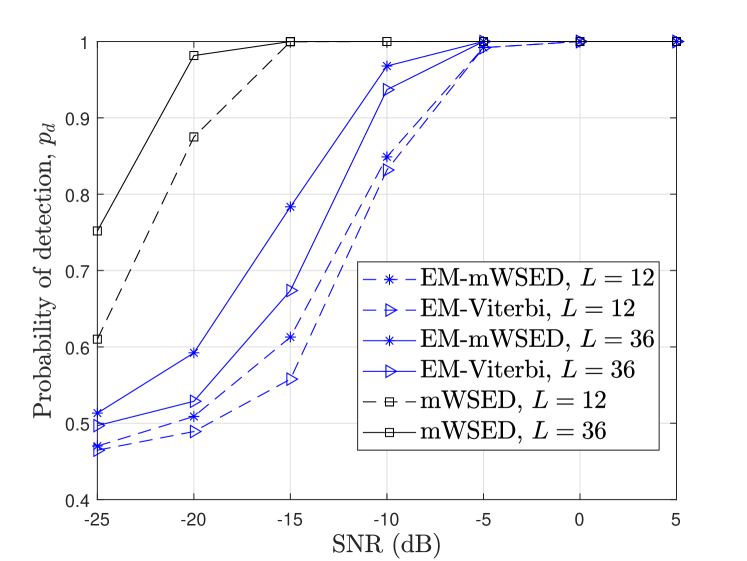
In general, a poor estimation error for PU’s states do effect the detection performances of EM-Viterbi444Since the last element in the state vector estimate, at SU , represents an estimate of the PU’s state in the present sensing period , EM-Viterbi can also be used for PU detection. and EM-mWSED schemes, but for an appropriate choice of value and by aggregating present and past ED samples, we can improve the detection performance at lower SNRs. To illustrate this fact, in Fig. 7, we compare the detection performances of EM-Viterbi and EM-mWSED by varying SNR and values, when , , and . Note that the state vector estimated by EM-Viterbi is used in EM-mWSED to average the highly correlated present and past ED samples. The weights on the aggregated ED samples in EM-mWSED are chosen as exponentially distributed as it results in better detection performance than equal weighting at lower SNR or values, due to the rise in the estimation error. Further, the threshold at each SNR and values is selected based on the false alarm rate of EM-Viterbi. However, it is observed that the detection performance of EM-mWSED is better than that of EM-Viterbi at lower SNRs, and that the performance of EM-mWSED improves significantly by a slight increase in the value. While the increase in aids in improving the EM’s estimation performance, the better performance of mWSED is due to the fact that it averages the highly correlated present and past ED samples in its test statistics which reduces the variances under the two hypotheses as illustrated in Section III-D. This improves the detection performance at lower SNRs and smaller values. Finally, as expected, we also observe that the performances of both algorithms achieve that of mWSED with an increase in SNR or values.
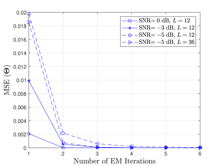
In Fig. 8, we illustrate the convergence performance of the EM algorithm in estimating the model parameters when SUs are considered in the network with network connectivity . The mean-squared error (MSE) of is defined as . It is observed that for samples per energy statistics, as the SNR increase from dB, to dB, and then to dB, the EM algorithm converges faster in fewer iterations. Similar observation is also made when for a lower SNR value of dB, we increase from to . This is due to the fact that the initial estimates for EM are improved at the larger SNR and values which results in its faster convergence response and improved estimation performance.
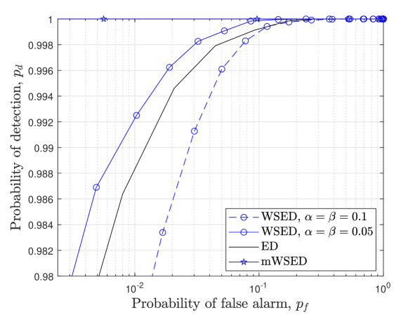
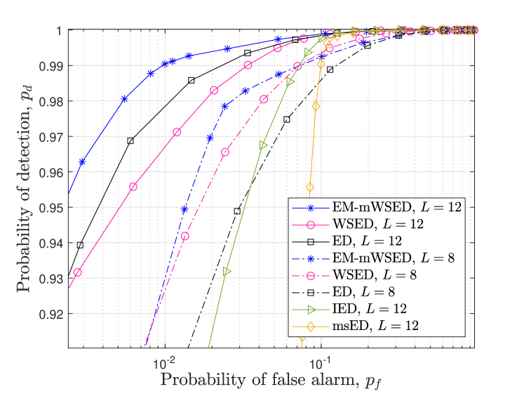
While EM-Viterbi provides a single operating point for SUs due to the estimation of the present state, in terms of detection probability and false alarm probability; in contrast, by using the estimated state vector in mWSED, the EM-mWSED algorithm can provide a wide range of operating points for SUs. Further, as observed in Fig. 7, EM-mWSED outperforms EM-Viterbi at lower SNRs which makes it a preferable choice. As such, in Figs. 9 and 10, we show the receiver operating characteristic (ROC) curves of the proposed EM-mWSED algorithm and compare it with those of the ED, WSED, IED, and msED schemes. In Fig. 9, we consider SUs in the network with connectivity . The PU states transitioning probabilities are selected as . The SNR is assumed to be dB, whereas the number of samples per energy statistic is assumed to be either or . As expected, it is observed that EM-mWSED outperforms all other methods at increasing the detection probability and reducing the false alarm probability, and thereby provides a wide range of operating points for SU. Furthermore, the detection performance of EM-mWSED improves with the increase in the values, due to decrease in the states estimation error.
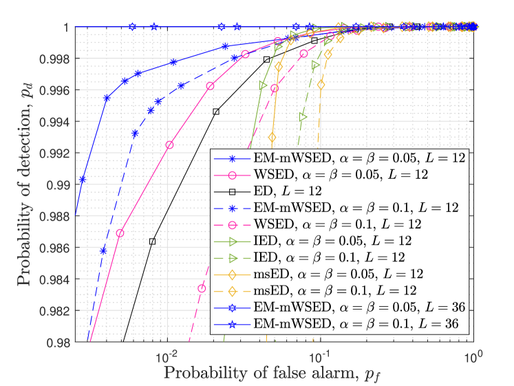
Fig. 10 compares the ROC curves of EM-mWSED with that of ED, WSED, IED, and msED schemes. The PU is either considered to be slowly time-varying with or highly dynamic with as considered earlier. There are SUs in the network with connectivity , and the SNR is considered to be dB with the number of samples per energy statistics as either or . Firstly, by comparing Figs. 9 and 10 for , SNR dB, and , we observe a decay in the detection performance of EM-mWSED due to decrease in the value of in Fig. 10, which reduces the SNR upon consensus as discussed above. Secondly, it is observed in Fig. 10 that for both slowly and highly dynamic natures of the PU, our EM-mWSED algorithm performs better than the other detectors as expected. However, when , its detection performance appears to be dependent on the time-varying nature of the PU, and it is seen to be better in case of slowly time-varying PU than a highly dynamic PU. This is because at the lower SNR or values, EM-Viterbi can easily characterize the ED samples, corresponding to the two states of PU, when the PU is slowly time-varying than when it is highly dynamic, and thus results in a lower estimation error in the former case. However, when increases to , then the estimation error of EM-Viterbi decreases for a highly dynamic PU as well, which in turn results in the similar performance of EM-mWSED for both kinds of PUs, as shown in this figure.
Finally, while the focus herein is on investigating the detection vs. false alarm probabilities, it is worth noting that, on the one hand, where the throughput performance of an SU under is proportional to , on the other hand, the throughput under is proportional to [40]. Thus, the higher detection probability of EM-mWSED as compared with that of ED, WSED, IED, and msED implies a higher throughput of SUs with reduced interference to the primary user, whereas its capability of simultaneously decreasing the false alarm probability with the increase in the average connections per SUs in the network, SNR, or , implies a higher throughput during the idle state of the PU.
VI Conclusion
We considered the problem of DCSS at lower SNRs when the present and past ED samples are aggregated in a test statistic for improved PU detection with fewer samples per energy statistics. Using a few samples per energy aids in reducing the sensing duration and power consumption per SU. Furthermore, it increases the throughput of the network. A modified weighted sequential energy detector is proposed which utilizes the PU states information over an observation window to combine only the highly correlated ED samples in its test statistics. In practice, the states information is unknown, and thus we developed an EM-Viterbi algorithm to iteratively estimate them using the ED samples collected over the window. The estimated states are then used in mWSED to compute its test statistics, and the resulting algorithm is named here as the EM-mWSED algorithm. Simulation results are included to demonstrate the estimation performance of EM-Viterbi and compare the detection performance of both EM-Viterbi and EM-mWSED schemes. Furthermore, the detection performance of EM-mWSED is compared with that of the conventional ED, WSED, IED, and msED methods. The results demonstrate that our proposed EM-mWSED performs better than the other schemes, and its performance improves by either increasing the average number of connections per SU in the network, or by increasing the SNR or the number of samples per energy statistics, for both slowly varying and highly dynamic PU.
Herein, we present the derivation of the probabilities and for and the -th iteration of EM. To begin, the posterior distribution of given and can be written as
| (25) |
where the distributions and are computed later herein. The notation which is a shorthand to represent the elements in from index to where . Similarly, we can write the joint distribution of and as
| (26) |
where the conditional distribution of and the conditional prior distribution of that are used above are both defined in (10) and (IV). Next we follow the forward-backward recursion approach in [37] to compute the distributions and . First, to compute , we write
| (27) |
where we have defined , and in (VI) the summation is over . The forward recursion in (VI) occurs in the -iteration of EM for all with the initialization which is defined in (10) and (IV). Next we write the backward recursion equation to compute as follows
| (28) |
in which the summation runs over for all with the initialization . Finally, the probabilities and for can be computed as
| (29) |
and,
| (30) |
References
- [1] A. M. Voicu, L. Simić, and M. Petrova, “Survey of Spectrum Sharing for Inter-Technology Coexistence,” IEEE Communications Surveys & Tutorials, vol. 21, no. 2, pp. 1112–1144, 2019.
- [2] L. Liu, C. Masouros, and A. L. Swindlehurst, “Robust Symbol Level Precoding for Overlay Cognitive Radio Networks,” IEEE Transactions on Wireless Communications, vol. 23, no. 2, pp. 1403–1415, 2024.
- [3] S. Haykin, “Cognitive radio: brain-empowered wireless communications,” IEEE Journal on Selected Areas in Communications, vol. 23, no. 2, pp. 201–220, 2005.
- [4] F. F. Digham, M.-S. Alouini, and M. K. Simon, “On the Energy Detection of Unknown Signals Over Fading Channels,” IEEE Transactions on Communications, vol. 55, no. 1, pp. 21–24, 2007.
- [5] F. Moghimi, R. Schober, and R. K. Mallik, “Hybrid Coherent/Energy Detection for Cognitive Radio Networks,” IEEE Transactions on Wireless Communications, vol. 10, no. 5, pp. 1594–1605, 2011.
- [6] U. Salama, P. L. Sarker, and A. Chakrabarty, “Enhanced Energy Detection using Matched Filter for Spectrum Sensing in Cognitive Radio Networks,” in 2018 Joint 7th International Conference on Informatics, Electronics & Vision (ICIEV) and 2018 2nd International Conference on Imaging, Vision & Pattern Recognition (icIVPR), 2018, pp. 185–190.
- [7] A. Bagwari and G. S. Tomar, “Multiple Energy Detection vs Cyclostationary Feature Detection Spectrum Sensing Technique,” in 2014 Fourth International Conference on Communication Systems and Network Technologies, 2014, pp. 178–181.
- [8] W. M. Jang, “Simultaneous Power Harvesting and Cyclostationary Spectrum Sensing in Cognitive Radios,” IEEE Access, vol. 8, pp. 56 333–56 345, 2020.
- [9] R. Wang and M. Tao, “Blind Spectrum Sensing by Information Theoretic Criteria for Cognitive Radios,” IEEE Transactions on Vehicular Technology, vol. 59, no. 8, pp. 3806–3817, 2010.
- [10] S. M. Hiremath, S. K. Patra, T. P. Sahu, and A. K. Mishra, “Higher order eigenvalue-moment-ratio based blind spectrum sensing: Application to cognitive radio,” in TENCON 2017 - 2017 IEEE Region 10 Conference, 2017, pp. 2291–2296.
- [11] A. Sabra and M. Berbineau, “Experimental Assessment of Eigenvalue-Based Spectrum Sensing Using USRP-Based MIMO Testbed for Cognitive Radio Applications,” IEEE Sensors Letters, vol. 6, no. 10, pp. 1–4, 2022.
- [12] C. Vlădeanu, A. Marţian, and D. C. Popescu, “Spectrum Sensing With Energy Detection in Multiple Alternating Time Slots,” IEEE Access, vol. 10, pp. 38 565–38 574, 2022.
- [13] Q. Tian, Y. Wu, F. Shen, F. Zhou, Q. Wu, and O. A. Dobre, “ED-Based Spectrum Sensing for the Satellite Communication Networks Using Phased-Array Antennas,” IEEE Communications Letters, vol. 27, no. 7, pp. 1834–1838, 2023.
- [14] M. López-Benítez and F. Casadevall, “Improved energy detection spectrum sensing for cognitive radio,” IET Communications, vol. 6, pp. 785–796(11), May 2012.
- [15] W. Prawatmuang, D. K. C. So, and E. Alsusa, “Sequential Cooperative Spectrum Sensing Technique in Time Varying Channel,” IEEE Transactions on Wireless Communications, vol. 13, no. 6, pp. 3394–3405, 2014.
- [16] W. Prawatmuang and D. K. C. So, “Adaptive sequential cooperative spectrum sensing technique in time varying channel,” in 2012 IEEE 23rd International Symposium on Personal, Indoor and Mobile Radio Communications - (PIMRC), 2012, pp. 1546–1551.
- [17] B. Kailkhura, S. Brahma, and P. K. Varshney, “Data Falsification Attacks on Consensus-Based Detection Systems,” IEEE Transactions on Signal and Information Processing over Networks, vol. 3, no. 1, pp. 145–158, 2017.
- [18] A. Ghasemi and E. Sousa, “Collaborative spectrum sensing for opportunistic access in fading environments,” in First IEEE International Symposium on New Frontiers in Dynamic Spectrum Access Networks, 2005. DySPAN 2005., 2005, pp. 131–136.
- [19] K. Cichoń, A. Kliks, and H. Bogucka, “Energy-Efficient Cooperative Spectrum Sensing: A Survey,” IEEE Communications Surveys & Tutorials, vol. 18, no. 3, pp. 1861–1886, 2016.
- [20] M. Najimi, A. Ebrahimzadeh, S. M. H. Andargoli, and A. Fallahi, “A Novel Sensing Nodes and Decision Node Selection Method for Energy Efficiency of Cooperative Spectrum Sensing in Cognitive Sensor Networks,” IEEE Sensors Journal, vol. 13, no. 5, pp. 1610–1621, 2013.
- [21] H. Kaschel, K. Toledo, J. T. Gómez, and M. J. F.-G. García, “Energy-Efficient Cooperative Spectrum Sensing Based on Stochastic Programming in Dynamic Cognitive Radio Sensor Networks,” IEEE Access, vol. 9, pp. 720–732, 2021.
- [22] Z. Li, F. R. Yu, and M. Huang, “A Distributed Consensus-Based Cooperative Spectrum-Sensing Scheme in Cognitive Radios,” IEEE Transactions on Vehicular Technology, vol. 59, no. 1, pp. 383–393, 2010.
- [23] A. Mustafa, M. N. U. Islam, and S. Ahmed, “Dynamic Spectrum Sensing Under Crash and Byzantine Failure Environments for Distributed Convergence in Cognitive Radio Networks,” IEEE Access, vol. 9, pp. 23 153–23 167, 2021.
- [24] A. Gharib, W. Ejaz, and M. Ibnkahla, “Enhanced Multiband Multiuser Cooperative Spectrum Sensing for Distributed CRNs,” IEEE Transactions on Cognitive Communications and Networking, vol. 6, no. 1, pp. 256–270, 2020.
- [25] R. Olfati-Saber, J. A. Fax, and R. M. Murray, “Consensus and Cooperation in Networked Multi-Agent Systems,” Proceedings of the IEEE, vol. 95, no. 1, pp. 215–233, 2007.
- [26] S. Boyd, P. Diaconis, and L. Xiao, “Fastest Mixing Markov Chain on a Graph,” SIAM Review, vol. 46, no. 4, pp. 667–689, 2004.
- [27] H. Wang, W. Xu, and J. Lu, “Privacy-Preserving Push-sum Average Consensus Algorithm over Directed Graph Via State Decomposition,” in 2021 3rd International Conference on Industrial Artificial Intelligence (IAI), 2021, pp. 1–6.
- [28] X. Qiao, Y. Wu, and D. Meng, “Privacy-Preserving Average Consensus for Multi-agent Systems with Directed Topologies,” in 2021 8th International Conference on Information, Cybernetics, and Computational Social Systems (ICCSS), 2021, pp. 7–12.
- [29] A. Moradi, N. K. D. Venkategowda, and S. Werner, “Total Variation-Based Distributed Kalman Filtering for Resiliency Against Byzantines,” IEEE Sensors Journal, vol. 23, no. 4, pp. 4228–4238, 2023.
- [30] X. Liu, K. Zheng, K. Chi, and Y.-H. Zhu, “Cooperative Spectrum Sensing Optimization in Energy-Harvesting Cognitive Radio Networks,” IEEE Transactions on Wireless Communications, vol. 19, no. 11, pp. 7663–7676, 2020.
- [31] G. Forney, “The viterbi algorithm,” Proceedings of the IEEE, vol. 61, no. 3, pp. 268–278, 1973.
- [32] J. Proakis and M. Salehi, Digital Communications, 5th edition. McGraw-Hill Higher Education, 2008.
- [33] J. Gubner, Probability and Random Processes for Electrical and Computer Engineers. Cambridge University Press, 2006.
- [34] S. Boyd and L. Vandenberghe, Convex Optimization, ser. Berichte über verteilte messysteme. Cambridge University Press, 2004, no. pt. 1.
- [35] A. P. Dempster, N. M. Laird, and D. B. Rubin, “Maximum likelihood from incomplete data via the EM algorithm,” Journal of the Royal Statistical Society, Series B, vol. 39, no. 1, pp. 1–38, 1977.
- [36] C. M. Bishop, Pattern Recognition and Machine Learning (Information Science and Statistics). Secaucus, NJ, USA: Springer-Verlag New York, Inc., 2006.
- [37] L. E. Baum, T. Petrie, G. Soules, and N. Weiss, “A Maximization Technique Occurring in the Statistical Analysis of Probabilistic Functions of Markov Chains,” The Annals of Mathematical Statistics, vol. 41, no. 1, pp. 164–171, 1970.
- [38] M. Rashid and M. Naraghi-Pour, “Multitarget Joint Delay and Doppler-Shift Estimation in Bistatic Passive Radar,” IEEE Transactions on Aerospace and Electronic Systems, vol. 56, no. 3, pp. 1795–1806, 2020.
- [39] M. Rashid and J. A. Nanzer, “Online Expectation-Maximization Based Frequency and Phase Consensus in Distributed Phased Arrays,” IEEE Transactions on Communications, pp. 1–1, 2023.
- [40] R. A. Rashid, Y. S. Baguda, N. Fisal, M. Adib Sarijari, S. K. S. Yusof, S. H. S. Ariffin, N. M. A. Latiff, and A. Mohd, “Optimizing distributed cooperative sensing performance using swarm intelligence,” in Informatics Engineering and Information Science. Springer, Berlin, Heidelberg, 2011, pp. 407–420.