Expected Sliced Transport Plans

Xinran Liu¹ Rocío Martín Díaz² Yikun Bai¹ Ashkan Shahbazi¹
Matthew Thorpe³ Akram Aldroubi⁴ Soheil Kolouri¹

¹Department of Computer Science Vanderbilt University Nashville TN 3723
²Department of Mathematics Tufts University Medford MA 02155
³Department of Statistics University of Warwick Coventry CV4 7AL UK
⁴Department of Mathematics Vanderbilt University Nashville TN 3723

Abstract

The optimal transport (OT) problem has gained significant traction in modern machine learning for its ability to: (1) provide versatile metrics, such as Wasserstein distances and their variants, and (2) determine optimal couplings between probability measures. To reduce the computational complexity of OT solvers, methods like entropic regularization and sliced optimal transport have been proposed. The sliced OT framework improves efficiency by comparing one-dimensional projections (slices) of high-dimensional distributions. However, despite their computational efficiency, sliced-Wasserstein approaches lack a transportation plan between the input measures, limiting their use in scenarios requiring explicit coupling. In this paper, we address two key questions: Can a transportation plan be constructed between two probability measures using the sliced transport framework? If so, can this plan be used to define a metric between the measures? We propose a "lifting" operation to extend one-dimensional optimal transport plans back to the original space of the measures. By computing the expectation of these lifted plans, we derive a new transportation plan, termed expected sliced transport (EST) plans. We prove that using the EST plan to weight the sum of the individual Euclidean costs for moving from one point to another results in a valid metric between the input discrete probability measures. We demonstrate the connection between our approach and the recently proposed min-SWGG, along with illustrative numerical examples that support our theoretical findings.

1 Introduction

The optimal transport (OT) problem (Villani, 2009) seeks the most efficient way to transport a distribution of mass from one configuration to another, minimizing the cost associated with the transportation process. It has found diverse applications in machine learning due to its ability to provide meaningful distances, i.e., the Wasserstein distances (Peyré & Cuturi, 2019), between probability distributions, with applications ranging from supervised learning (Frogner et al., 2015) to generative modeling (Arjovsky et al., 2017). Beyond merely measuring distances between probability measures, the optimal transportation plan obtained from the OT problem provides correspondences between the empirical samples of the source and target distributions, which are used in various applications, including domain adaptation (Courty et al., 2014), positive-unlabeled learning (Chapel et al., 2020), texture mixing (Rabin et al., 2011), color transfer (Rabin et al., 2014), image analysis (Basu et al., 2014), and even single-cell and spatial omics (Bunne et al., 2024), to name a few.

One of the primary challenges in applying the OT framework to large-scale problems is its computational complexity. Traditional OT solvers for discrete measures typically scale cubically with the number of samples (i.e., the support size) (Kolouri et al., 2017). This computational burden has spurred significant research efforts to accelerate OT computations. Various approaches have been developed to address this challenge, including entropic regularization (Cuturi, 2013), multiscale methods (Schmitzer, 2016), and projection-based techniques such as sliced-Wasserstein distances (Rabin et al., 2011) and robust subspace OT (Paty & Cuturi, 2019). Each of these methods has its own advantages and limitations.

For instance, the entropic regularized OT is solved via an iterative algorithm (i.e., the Sinkhorn algorithm) with quadratic computational complexity per iteration. However, the number of iterations required for convergence typically increases as the regularization parameter decreases, which can offset the computational benefits of these methods. Additionally, while entropic regularization interpolates between Maximum-Mean Discrepancy (MMD) (Gretton et al., 2012) and the Wasserstein distance (Feydy et al., 2019), it does not produce a true metric between probability measures. Despite not providing a metric, the entropic OT provides a transportation plan, i.e., soft correspondences, albeit not the optimal one. On the other hand, sliced-Wasserstein distances offer linearithmic computational complexity, enabling the comparison of discrete measures with millions of samples. These distances are also topologically equivalent to the Wasserstein distance and offer statistical advantages, such as better sample complexity (Nadjahi et al., 2020). However, despite their computational efficiency, the sliced-Wasserstein approaches do not provide a transportation plan between the input probability measures, limiting their applicability to problems that require explicit coupling between measures.

In this paper, we address two central questions: First, can a transportation plan be constructed between two probability measures using the sliced transport framework? If so, can the resulting transportation plan be used to define a metric between the two probability measures? Within the sliced transport framework, the "slices" refer to the one-dimensional marginals of the source and target probability measures, for which an optimal transportation plan is computed. Crucially, this optimal transportation plan applies to the marginals (i.e., one-dimensional probability measures) rather than the original measures. To derive a transportation plan between the source and target measures, this optimal plan for the marginals must be "lifted" back to the original space.

For discrete measures with equal support size, $N$ , and uniform mass, $1/N$ , the optimal transportation plan between marginals is represented by a correspondence matrix, specifically an $N\times N$ permutation matrix. Previous works have used directly the correspondence matrix obtained for a slice as a transportation plan in the original space of measures (Rowland et al., 2019; Mahey et al., 2023). This paper provides a holistic and rigorous analysis of this problem for general discrete probability measures.

Our specific contributions in this paper are:

1.

Introducing a computationally efficient transportation plan between discrete probability measures, the Expected Sliced Transport plan.
2.

Providing a distance for discrete probability measures, the Expected Sliced Transport (EST) distance.
3.

Offering both a theoretical proof and an experimental visualization showing that the EST distance is equivalent to the Wasserstein distance (and to weak^∗ convergence) when applied to discrete measures.
4.

Demonstrating the performance of the proposed distance and the transportation plan in diverse applications, namely interpolation and classification.

2 Expected Sliced Transport

2.1 Preliminaries

Given a probability measure $\mu\in\mathcal{P}(\mathbb{R}^{d})$ and a unit vector $\theta\in\mathbb{S}^{d-1}\subset\mathbb{R}^{d}$ , we define $\theta_{\#}\mu:=\langle\theta,\cdot\rangle_{\#}\mu$ to be the $\theta$ -slice of the measure $\mu$ , where $\langle\theta,x\rangle=\theta\cdot x=\theta^{T}x$ denotes the standard inner product in $\mathbb{R}^{d}$ . For any pair of probability measures with finite $p$ -moment ( $p>1$ ) $\mu^{1},\mu^{2}\in\mathcal{P}_{p}(\mathbb{R}^{d})$ , one can pose the following two Optimal Transport (OT) problems: On the one hand, consider the classical OT problem, which gives rise to the $p$ -Wasserstein metric:

\displaystyle W_{p}(\mu^{1},\mu^{2}):=\min_{\gamma\in\Gamma(\mu^{1},\mu^{2})}\left(\int_{\mathbb{R}^{d}\times\mathbb{R}^{d}}\|x-y\|^{p}d\gamma(x,y)\right)^{1/p}

(1)

where $\|\cdot\|$ denotes the Euclidean norm in $\mathbb{R}^{d}$ and $\Gamma(\mu^{1},\mu^{2})\subset\mathcal{P}(\mathbb{R}^{d}\times\mathbb{R}^{d})$ is the subset of all probability measures with marginals $\mu^{1}$ and $\mu^{2}$ . On the other hand, for a given $\theta\in\mathbb{S}^{d-1}$ , consider the one-dimensional OT problem:

\displaystyle W_{p}(\theta_{\#}\mu^{1},\theta_{\#}\mu^{2})=\min_{\Lambda_{\theta}\in\Gamma(\theta_{\#}\mu^{1},\theta_{\#}\mu^{2})}\left(\int_{\mathbb{R}\times\mathbb{R}}|u-v|^{p}d\Lambda_{\theta}(u,v)\right)^{1/p}

(2)

In this case, since the measures $\theta_{\#}\mu^{1},\theta_{\#}\mu^{2}$ can be regarded as one-dimensional probabilities in $\mathcal{P}(\mathbb{R})$ , there exists a unique optimal transport plan, which we denote by $\Lambda_{\theta}^{\mu_{1},\mu_{2}}$ (see, for e.g., (Villani, 2021, Thm. 2.18, Remark 2.19)], (Maggi, 2023, Thm. 16.1)).

2.2 On slicing and lifting transport plans

In this section, given discrete probability measures $\mu^{1},\mu^{2}\in\mathcal{P}(\mathbb{R}^{d})$ , we describe the process of slicing them according to a direction $\theta\in\mathbb{S}^{d-1}$ and lifting the optimal transportation plan $\Lambda_{\theta}^{\mu^{1},\mu^{2}}$ , which solves the 1-dimensional OT problem (2), to get a plan in $\Gamma(\mu^{1},\mu^{2})$ . Thus, we obtain a new measure, denoted as $\gamma_{\theta}^{\mu^{1},\mu^{2}}$ , in $\mathcal{P}(\mathbb{R}^{d}\times\mathbb{R}^{d})$ with first and second marginal $\mu^{1}$ and $\mu^{2}$ , respectively. For clarity, we first describe the process for discrete uniform measures and then extend it to any pair of discrete measures.

2.2.1 On slicing and lifting transport plans for uniform discrete measures

Given $N\in\mathbb{N}$ , consider the space $\mathcal{P}_{(N)}(\mathbb{R}^{d})$ of uniform discrete probability measures concentrated at $N$ particles in $\mathbb{R}^{d}$ , that is,

\mathcal{P}_{(N)}(\mathbb{R}^{d})=\left\{\frac{1}{N}\sum_{i=1}^{N}\delta_{x_{i}}~{}|~{}x_{i}\in\mathbb{R}^{d},~{}\forall i\in\{1,...,N\}\right\}.

Let $\mu^{1}=\frac{1}{N}\sum_{i=1}^{N}\delta_{x_{i}},\mu^{2}=\frac{1}{N}\sum_{j=1}^{N}\delta_{y_{j}}\in\mathcal{P}_{(N)}(\mathbb{R}^{d})$ , where $x_{i},y_{j}\in\mathbb{R}^{d}$ and $\delta_{x_{i}}$ denotes a Dirac measure located at $x_{i}$ (respectively for $\delta_{y_{j}}$ ). Let us denote by $\mathcal{U}(\mathbb{S}^{d-1})$ the uniform measure on the hypersphere $\mathbb{S}^{d-1}\subset\mathbb{R}^{d}$ . In this case, the $\theta$ -slice of $\mu^{1}$ is represented by $\theta_{\#}\mu^{1}=\frac{1}{N}\sum_{i=1}^{N}\delta_{\theta\cdot x_{i}}$ , and similarly for $\theta_{\#}\mu^{2}$ . Let $\mathbf{S}_{N}$ denote the symmetric group of all permutations of the elements in the set $[N]:=\{1,\dots,N\}$ . Let $\zeta_{\theta},\tau_{\theta}\in\mathbf{S}_{N}$ denote the sorted indices of the projected points $\{\theta\cdot x_{i}\}_{i=1}^{N}$ and $\{\theta\cdot y_{j}\}_{j=1}^{N}$ , respectively, that is,

\theta\cdot x_{\zeta_{\theta}^{-1}(1)}\leq\theta\cdot x_{\zeta_{\theta}^{-1}(2)}\leq\dots\leq\theta\cdot x_{\zeta_{\theta}^{-1}(N)}\text{ and }\theta\cdot y_{\tau_{\theta}^{-1}(1)}\leq\theta\cdot y_{\tau_{\theta}^{-1}(2)}\leq\dots\leq\theta\cdot y_{\tau_{\theta}^{-1}(N)}

(3)

The optimal matching from $\theta_{\#}\mu^{1}$ to $\theta_{\#}\mu^{2}$ for the problem (2) is induced by the assignment

\theta\cdot x_{\zeta_{\theta}^{-1}(i)}\longmapsto\theta\cdot y_{\tau_{\theta}^{-1}(i)},\qquad\forall 1\leq i\leq N.

(4)

We define $T_{\theta}^{\mu^{1},\mu^{2}}:\{x_{1},\dots,x_{N}\}\to\{y_{1},\dots,y_{N}\}$ the lifted transport map between $\mu^{1}$ and $\mu^{2}$ by:

T_{\theta}^{\mu^{1},\mu^{2}}(x_{i})=y_{\tau^{-1}_{\theta}(\zeta_{\theta}(i))},\qquad\forall 1\leq i\leq N.

(5)

Rigorously, $T_{\theta}^{\mu^{1},\mu^{2}}$ is not necessarily a function defined on $\{x_{1},\dots,x_{N}\}$ but on the the labels $\{1,\dots,N\}$ , as two projected points $\theta\cdot x_{i}$ and $\theta\cdot x_{j}$ could coincide for $i\not=j$ . As a result, it is more convenient to work with lifted transport plans. Indeed, the matrix $u_{\theta}^{\mu^{1},\mu^{2}}\in\mathbb{R}^{n\times n}$ given by

u_{\theta}^{\mu^{1},\mu^{2}}(i,j)=\begin{cases}1/N&\text{if }j=\tau^{-1}_{\theta}(\zeta_{\theta}(i))\\ 0&\text{otherwise}\end{cases}

(6)

encodes the weights of optimal transport plan between $\theta_{\#}\mu^{1}$ and $\theta_{\#}\mu^{2}$ given by

\Lambda_{\theta}^{\mu^{1},\mu^{2}}:=\sum_{i,j}u_{\theta}^{\mu^{1},\mu^{2}}(i,j)\delta_{(\theta\cdot x_{i},\theta\cdot y_{j})},

(7)

as well as the weights of the lifted transport plan between the original measures $\mu^{1}$ and $\mu^{2}$ according to the $\theta$ -slice defined by

\gamma_{\theta}^{\mu^{1},\mu^{2}}:=\sum_{i,j}u_{\theta}^{\mu^{1},\mu^{2}}(i,j)\delta_{(x_{i},y_{j})}.

(8)

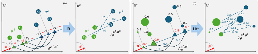
This new measure $\gamma_{\theta}^{\mu^{1},\mu^{2}}\in\mathcal{P}(\mathbb{R}^{d}\times\mathbb{R}^{d})$ has marginals $\mu^{1}$ and $\mu^{2}$ . While $\gamma_{\theta}^{\mu^{1},\mu^{2}}$ is not necessarily optimal for the OT problem (1) between $\mu^{1}$ and $\mu^{2}$ , it can be interpreted as a transport plan in $\Gamma(\mu^{1},\mu^{2})$ which is optimal when projecting $\mu^{1}$ and $\mu^{2}$ in the direction of $\theta$ . See Figure 1 (a) for a visualization.

Refer to caption — Figure 1: Visualization of the 1-dimensional plan $\Lambda_{\theta}^{\mu^{1},\mu^{2}}$ (given an unit vector $\theta$ ) and the corresponding lifted transport plan $\gamma_{\theta}^{\mu^{1},\mu^{2}}$ between discrete probability measures $\mu^{1}$ (green circles) and $\mu^{2}$ (blue circles). In (a) the measures $\mu^{1},\mu^{2}$ are uniform and the masses do not overlap when projecting in the direction of $\theta$ . In (b) the measures $\mu^{1},\mu^{2}$ are not uniform and some of the masses overlap when projecting in the direction of $\theta$ . For more details see Remark A.1 in Appendix A.1.

2.2.2 On slicing and lifting transport plans for general discrete measures

Consider discrete measures $\mu^{1},\mu^{2}\in\mathcal{P}(\mathbb{R}^{d})$ . In this section, we will use the notation $\mu^{1}=\sum_{x\in\mathbb{R}^{d}}p(x)\delta_{x}$ , where $p(x)\geq 0$ for all $x\in\mathbb{R}^{d}$ , $p(x)\not=0$ for at most countable many points $x\in\mathbb{R}^{d}$ , and $\sum_{x\in\mathbb{R}^{d}}p(x)=1$ . Similarly, $\mu^{2}=\sum_{y\in\mathbb{R}^{d}}q(y)\delta_{y}$ for a non-negative density function $q$ in $\mathbb{R}^{d}$ with finite or countable support and such that $\sum_{y\in\mathbb{R}^{d}}q(y)=1$ . Given $\theta\in\mathbb{S}^{d-1}$ , consider the equivalence relation defined by:

x\sim_{\theta}x^{\prime}\quad\text{ if and only if }\quad\theta\cdot x=\theta\cdot x^{\prime}

We denote by $\bar{x}^{\theta}$ the equivalence class of $x\in\mathbb{R}^{d}$ . By abuse of notation, we will use interchangeably that $\bar{x}^{\theta}$ is a point in the quotient space $\mathbb{R}^{d}/{\sim_{\theta}}$ , and also the set $\{x^{\prime}\in\mathbb{R}^{d}:\ \theta\cdot x=\theta\cdot x^{\prime}\}$ , which is the orthogonal hyperplane to $\theta$ that intersects $x$ . The intended meaning of $\bar{x}^{\theta}$ will be clear from the context. Notice that, geometrically, the quotient space $\mathbb{R}^{d}/{\sim_{\theta}}$ is the line $\mathbb{R}$ in the direction of $\theta$ .

Now, we interpret the projected measures $\theta_{\#}\mu^{1}$ , $\theta_{\#}\mu^{2}$ as 1-dimensional probability measures in $\mathcal{P}(\mathbb{R}^{d}/{\sim_{\theta}})$ given by $\theta_{\#}\mu^{1}=\sum_{\bar{x}^{\theta}\in\mathbb{R}^{d}/{\sim_{\theta}}}P(\bar{x}^{\theta})\delta_{\bar{x}^{\theta}}$ , where $P(\bar{x}^{\theta})=\sum_{x^{\prime}\in\bar{x}^{\theta}}p(x^{\prime})$ , and similarly, $\theta_{\#}\mu^{2}=\sum_{\bar{y}^{\theta}\in\mathbb{R}^{d}/{\sim_{\theta}}}Q(\bar{y}^{\theta})\delta_{\bar{y}^{\theta}}$ , where $Q(\bar{y}^{\theta})=\sum_{y^{\prime}\in\bar{y}^{\theta}}q(y^{\prime})$ .

Remark 2.1.

Notice that if $P(\bar{x}^{\theta})=0$ , then $p(x^{\prime})=0$ for all $x^{\prime}\in\bar{x}^{\theta}$ , or, equivalently, if $p(x)\not=0$ , then $P(\bar{x}^{\theta})\not=0$ (where $x$ is any ‘representative’ of the class $\bar{x}^{\theta}$ ). Similarly for $Q$ .

Consider the optimal transport plan $\Lambda_{\theta}^{\mu^{1},\mu^{2}}\in\Gamma(\theta_{\#}\mu^{1},\theta_{\#}\mu^{2})\subset\mathcal{P}(\mathbb{R}^{d}/{\sim_{\theta}}\times\mathbb{R}^{d}/{\sim_{\theta}})$ between $\theta_{\#}\mu^{1}$ and $\theta_{\#}\mu^{2}$ , which is unique for the OT problem (2) as we are considering 1-dimensional probability measures. Let us define

u_{\theta}^{\mu^{1},\mu^{2}}(x,y):=\begin{cases}\frac{p(x)q(y)}{P(\bar{x}^{\theta})Q(\bar{y}^{\theta})}\Lambda_{\theta}^{\mu^{1},\mu^{2}}(\{(\bar{x}^{\theta},\bar{y}^{\theta})\})&\text{ if }p(x)\not=0\text{ and }q(y)\not=0\\ 0&\text{ if }p(x)=0\text{ or }q(y)=0\end{cases}

which allows us to generalize the lifted transport plan given in (6) in the general discrete case:

\gamma_{\theta}^{\mu^{1},\mu^{2}}:=\sum_{x\in\mathbb{R}^{d}}\sum_{y\in\mathbb{R}^{d}}u_{\theta}^{\mu^{1},\mu^{2}}(x,y)\delta_{(x,y)}

(9)

See Figure 1 (b) for a visualization.

Remark 2.2.

Notice that this lifting process can be performed by starting with any transport plan $\Lambda_{\theta}\in\Gamma(\theta_{\#}\mu^{1},\theta_{\#}\mu^{2})$ , but in this article we will always consider the optimal transportation plan, i.e., $\Lambda_{\theta}=\Lambda_{\theta}^{\mu^{1},\mu^{2}}$ . The reason why we make this choice if because this will give rise to a metric between discrete probability measures: The EST distance which will be defined in Section 2.3.

Lemma 2.3.

Given general discrete probability measures $\mu^{1}$ and $\mu^{2}$ in $\mathbb{R}^{d}$ , the discrete measure $\gamma_{\theta}^{\mu^{1},\mu^{2}}$ defined by (9) has marginals $\mu^{1}$ and $\mu^{2}$ , that is, $\gamma_{\theta}^{\mu^{1},\mu^{2}}\in\Gamma(\mu^{1},\mu^{2})\subset\mathcal{P}(\mathbb{R}^{d}\times\mathbb{R}^{d})$ .

We refer the reader to the appendix for its proof.

2.3 Expected Sliced Transport (EST) for discrete measures

Leveraging on the transport plans $\gamma_{\theta}^{\mu^{1},\mu^{2}}$ described before, in this section we propose a new transportation plan $\bar{\gamma}^{\mu^{1},\mu^{2}}\in\Gamma(\mu^{1},\mu^{2})$ , which will give rise to a new metric in the space of discrete probability measures.

Definition 2.4 (Expected Sliced Transport plan).

Let $\sigma\in\mathcal{P}(\mathbb{S}^{d-1})$ . For discrete probability measures $\mu^{1},\mu^{2}$ in $\mathbb{R}^{d}$ , we define the expected sliced transport plan $\bar{\gamma}^{\mu^{1},\mu^{2}}\in\mathcal{P}(\mathbb{R}^{d}\times\mathbb{R}^{d})$ by

\bar{\gamma}^{\mu^{1},\mu^{2}}:=\mathbb{E}_{\theta\sim\sigma}[\gamma_{\theta}^{\mu^{1},\mu^{2}}],\qquad\text{ where each }\gamma_{\theta}^{\mu^{1},\mu^{2}}\text{ is given by }(\ref{eq: gamma theta for general discrete}),

(10)

that is,

\displaystyle\bar{\gamma}^{\mu^{1},\mu^{2}}(\{(x,y)\})=\int_{\mathbb{S}^{d-1}}\gamma_{\theta}^{\mu^{1},\mu^{2}}(\{(x,y)\})d\sigma(\theta),\qquad\forall x,y\in\mathbb{R}^{d}\times\mathbb{R}^{d}.

In other words, $\bar{\gamma}^{\mu^{1},\mu^{2}}=\sum_{x\in\mathbb{R}^{d}}\sum_{y\in\mathbb{R}^{d}}U^{\mu^{1},\mu^{2}}(x,y)\delta_{(x,y)}$ , where the new weights are given by

U^{\mu^{1},\mu^{2}}(x,y)=\begin{cases}p(x)q(y)\int_{\mathbb{S}^{d-1}}\frac{\Lambda_{\theta}^{\mu^{1},\mu^{2}}(\{(\bar{x}^{\theta},\bar{y}^{\theta})\})}{P(\bar{x}^{\theta})Q(\bar{y}^{\theta})}d\sigma(\theta)&\text{ if }p(x)\not=0\text{ and }q(y)\not=0\\ 0&\text{ otherwise}\end{cases}

Remark 2.5.

The measure $\bar{\gamma}^{\mu^{1},\mu^{2}}$ is well-defined and, moreover, (as an easy consequence of Lemma 2.3) $\bar{\gamma}^{\mu^{1},\mu^{2}}\in\Gamma(\mu^{1},\mu^{2})$ , i.e., it has marginals $\mu^{1}$ and $\mu^{2}$ . (See also Lemma A.5 in the appendix.)

Definition 2.6 (Expected Sliced Transport distance).

Let $\sigma\in\mathcal{P}(\mathbb{S}^{d-1})$ with $\mathrm{supp}(\sigma)=\mathbb{S}^{d-1}$ . We define the Expected Sliced Transport discrepancy for discrete probability measures $\mu^{1}$ , $\mu^{2}$ in $\mathbb{R}^{d}$ by

\displaystyle\mathcal{D}_{p}(\mu^{1},\mu^{2})

\displaystyle:=\left(\sum_{x\in\mathbb{R}^{d}}\sum_{y\in\mathbb{R}^{d}}\|x-y\|^{p}\,\bar{\gamma}^{\mu^{1},\mu^{2}}(\{(x,y)\})\right)^{1/p},

(11)

where $\bar{\gamma}^{\mu^{1},\mu^{2}}$ is defined by (10).

Remark 2.7.

By defining the following generalization of the Sliced Wasserstein Generalized Geodesics (SWGG) dissimilarity presented in Mahey et al. (2023),

\mathcal{D}_{p}(\mu^{1},\mu^{2};\theta):=\left(\sum_{x\in\mathbb{R}^{d}}\sum_{y\in\mathbb{R}^{d}}\|x-y\|^{p}\gamma_{\theta}^{\mu^{1},\mu^{2}}(\{x,y\})\right)^{1/p},

(12)

we can rewrite (11) as

\mathcal{D}_{p}(\mu^{1},\mu^{2})=\mathbb{E}^{1/p}_{\theta\sim\sigma}[\mathcal{D}^{p}_{p}(\mu^{1},\mu^{2};\theta)]

Remark 2.8.

Since the EST plan $\bar{\gamma}^{\mu^{1},\mu^{2}}$ is a transportation plan, we have that

W_{p}(\mu^{1},\mu^{2})\leq\mathcal{D}_{p}(\mu^{1},\mu^{2}).

In Appendix B we will show that they define the same topology in the space of discrete probability measures.

Remark 2.9 (EST for discrete uniform measures and the Projected Wasserstein distance).

Consider uniform measures $\mu^{1}=\frac{1}{N}\sum_{i=1}^{N}\delta_{x_{i}},\mu^{2}=\frac{1}{N}\sum_{j=1}^{N}\delta_{y_{j}}\in\mathcal{P}_{(N)}(\mathbb{R}^{d})$ , and for $\theta\in\mathbb{S}^{d-1}$ , let $\zeta_{\theta},\tau_{\theta}\in\mathbf{S}_{N}$ be permutations that allow us to order the projected points as in (3). Notice that if $\sigma=\mathcal{U}(\mathbb{S}^{d-1})$ , by using the formula (5) for each assignment given $\theta$ and noticing that $\tau_{\theta}^{-1}\circ\zeta_{\theta}\in\mathbf{S}_{N}$ , we can re-write (11) as

\mathcal{D}_{p}(\mu^{1},\mu^{2})^{p}=\mathbb{E}_{\theta\sim\mathcal{U}(\mathbb{S}^{d-1})}\left[\frac{1}{N}\sum_{i=1}^{N}\|x_{i}-y_{\tau^{-1}_{{\theta}}(\zeta_{\theta}(i))}\|^{p}\right].

(13)

Therefore, we have that the expression for $\mathcal{D}_{p}(\cdot,\cdot)$ given by (13) coincides with the Projected Wasserstein distance proposed in (Rowland et al., 2019, Definition 3.1). Then, by applying (Rowland et al., 2019, Proposition 3.3), we have that the Expected Sliced Transport discrepancy defined in Equation (13) is a metric on the space $\mathcal{P}_{(N)}(\mathbb{R}^{d})$ . We generalise this in the next theorem.

Theorem 2.10.

The Expected Sliced Transport $\mathcal{D}_{p}(\cdot,\cdot)$ defined in (11) is a metric in the space of finite discrete probability measures in $\mathbb{R}^{d}$ .

Sketch of the proof of Theorem 2.10.

For the detailed proof, we refer the reader to Appendix A. Here, we present a brief overview of the main ideas and steps involved in the proof.

The symmetry of $\mathcal{D}_{p}(\cdot,\cdot)$ follows from our construction of the transport plan $\bar{\gamma}^{\mu^{1},\mu^{2}}$ , which is based on considering a family of optimal 1-d transport plans $\{\Lambda_{\theta}^{\mu^{1},\mu^{2}}\}_{\theta\in\mathbb{S}^{d-1}}$ . The identity of indiscernibles follows essentially from Remark 2.8. To prove the triangle inequality we use the following strategy:

1.

We leverage the fact that $\mathcal{D}_{p}(\cdot,\cdot)$ is a metric for the space $\mathcal{P}_{(N)}(\mathbb{R}^{d})$ of uniform discrete probability measures concentrated at $N$ particles in $\mathbb{R}^{d}$ (Rowland et al. (2019)) to prove that $\mathcal{D}_{p}(\cdot,\cdot)$ is also a metric on the set of measures in which the masses are rationals. To do so, we establish a correspondence between finite discrete measures with rational weights and finite discrete measures with uniform mass (see the last paragraph of Proposition A.7).
2.
Given finite discrete measures $\mu^{1},\mu^{2}$ , we approximate them, in terms of the Total Variation norm, by sequences of probability measures with rational weights $\{\mu^{1}_{n}\},\{\mu^{2}_{n}\},$ supported on the same points as $\mu^{1}$ and $\mu^{2}$ , respectively. We then turn our attention on how the various plans constructed behave as the $n$ increases and show the following convergence results in Total Variation norm:
1. (a)
  
  The sequence $\left(\Lambda_{\theta}^{\mu^{1}_{n},\mu_{n}^{2}}\right)_{n\in\mathbb{N}}$ converges to $\Lambda_{\theta}^{\mu^{1},\mu^{2}}$ .
2. (b)
  
  The sequence $\left(\gamma_{\theta}^{\mu^{1}_{n},\mu_{n}^{2}}\right)_{n\in\mathbb{N}}$ converges to $\gamma_{\theta}^{\mu^{1},\mu^{2}}$ .
3. (c)
  
  The sequence $\left(\bar{\gamma}^{\mu_{n}^{1},\mu_{n}^{2}}\right)_{n\in\mathbb{N}}$ converges to $\bar{\gamma}^{\mu^{1},\mu^{2}}$ .
As a consequence, we obtain $\lim_{n\to\infty}\mathcal{D}_{p}(\mu_{n}^{1},\mu_{n}^{2})=\mathcal{D}_{p}(\mu^{1},\mu^{2}).$

Finally, given three finite discrete measures $\mu^{1},\mu^{2},\mu^{3}$ , we proceed as in point 2 by considering sequences of probability measures with rational weights $\{\mu^{1}_{n}\},\{\mu^{2}_{n}\},\{\mu^{3}_{n}\}$ supported on the same points as $\mu^{1}$ , $\mu^{2}$ , $\mu^{3}$ , respectively, that approximate the original measures in Total Variation, obtaining

\mathcal{D}_{p}(\mu^{1},\mu_{n}^{2})=\lim_{n\to\infty}\mathcal{D}_{p}(\mu_{n}^{1},\mu_{n}^{2})\leq\lim_{n\to\infty}\mathcal{D}_{p}(\mu_{n}^{1},\mu_{n}^{3})+\mathcal{D}_{p}(\mu^{3}_{n},\mu_{n}^{2})=\mathcal{D}_{p}(\mu^{1},\mu^{3})+\mathcal{D}_{p}(\mu^{3},\mu^{2})

where the equalities follows from point 2 and the middle triangle inequality follows from point 1. ∎

3 Experiments

3.1 Comparison of Transportation Plans

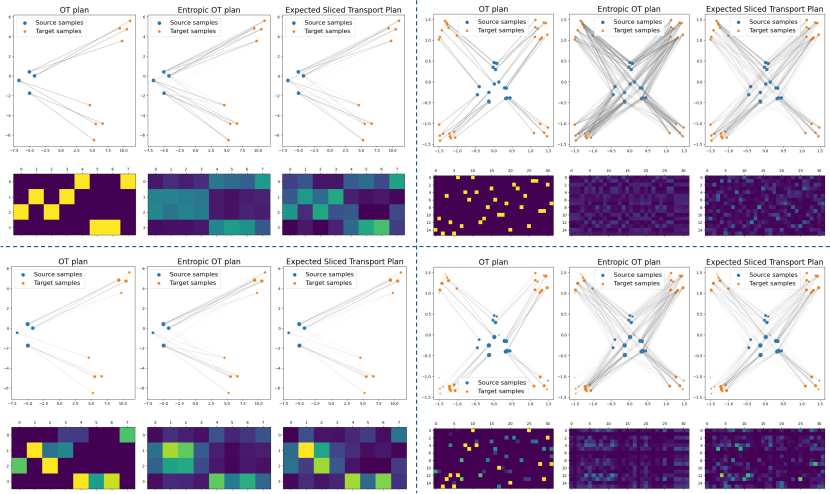
Figure 2 illustrates the behavior of different transport schemes: the optimal transport plan for $W_{2}(\cdot,\cdot)$ , the transport plan obtained by solving an entropically regularized transportation problem between the source and target probability measures, and the new expected sliced transport plan $\bar{\gamma}$ . We include comparisons with entropic regularization because it is one of the most popular approaches, as it allows for the use of Sinkhorn’s algorithm. From the figure, we observe that while $\bar{\gamma}$ promotes mass splitting, this phenomenon is less pronounced than in the entropically regularized OT scheme. This observation will be revisited in Subsection 3.2.

3.2 Temperature approach

Given $\mu^{1},\mu^{2}$ discrete probability measures, we perform the new expected sliced transportation scheme by using the following averaging measure $\sigma_{\tau}\ll\mathcal{U}(\mathbb{S}^{d-1})$ on the sphere:

d\sigma_{\tau}(\theta)=\frac{e^{-\tau\mathcal{D}^{p}_{p}(\mu^{1},\mu^{2};\theta)}}{\int_{\mathbb{S}^{d-1}}e^{-\tau\mathcal{D}_{p}^{p}(\mu^{1},\mu^{2};\theta^{\prime})}d\theta^{\prime}},

(14)

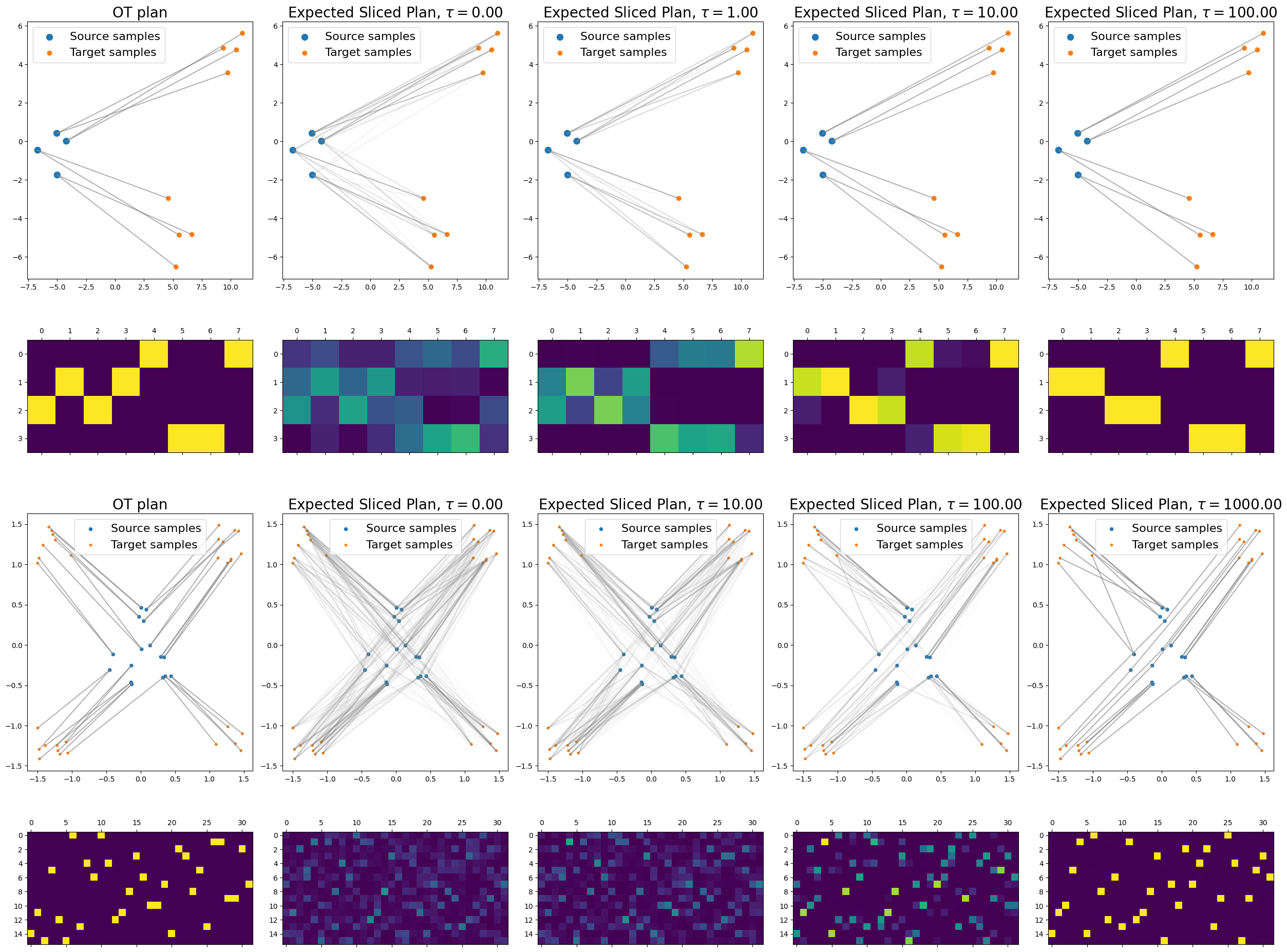
where $\mathcal{D}_{p}(\mu^{1},\mu^{2};\theta)$ is given by (12), and $\tau\geq 0$ is a hyperparameter we will refer to as the temperature (note that increasing $\tau$ corresponds to reducing the temperature). If $\tau=0$ , then $\sigma_{0}=\mathcal{U}(\mathbb{S}^{d-1})$ . However, when $\tau\neq 0$ , $\sigma_{\tau}$ is a probability measure on $\mathbb{S}^{d-1}$ with density given by (14), which depends on the source and target measures $\mu^{1}$ and $\mu^{2}$ . We have chosen this measure $\sigma_{\tau}$ because it provides a general parametric framework that interpolates between our proposed scheme with the uniform measure ( $\tau=0$ ) and min-SWGG (Mahey et al., 2023), as the EST distance approaches min-SWGG when $\tau\to\infty$ . For the implementations, we use

\sigma_{\tau}(\theta^{l})=\frac{e^{-\tau\mathcal{D}_{p}^{p}(\mu^{1},\mu^{2};\theta^{l})}}{\sum_{\ell^{\prime}=1}^{L}e^{-\tau\mathcal{D}_{p}^{p}(\mu^{1},\mu^{2};\theta^{\ell^{\prime}})}},

(15)

where $L$ represents the number of slices or unit vectors $\theta^{1},\dots,\theta^{L}\in\mathbb{S}^{d-1}$ . Figure 3 illustrates that as $\tau\to\infty$ , the weights used for averaging the lifted transportation plans converge to a one-hot vector, i.e., the slice minimizing $\mathcal{D}_{p}(\mu^{1},\mu^{2};\theta)$ dominates, leading to a transport plan with fewer mass splits. For the visualization we have used source $\mu^{1}$ and target $\mu^{2}$ uniform probability measures concentrated on different number of particles. For consistency, the configurations are the same as in Figure 2.

3.3 Interpolation

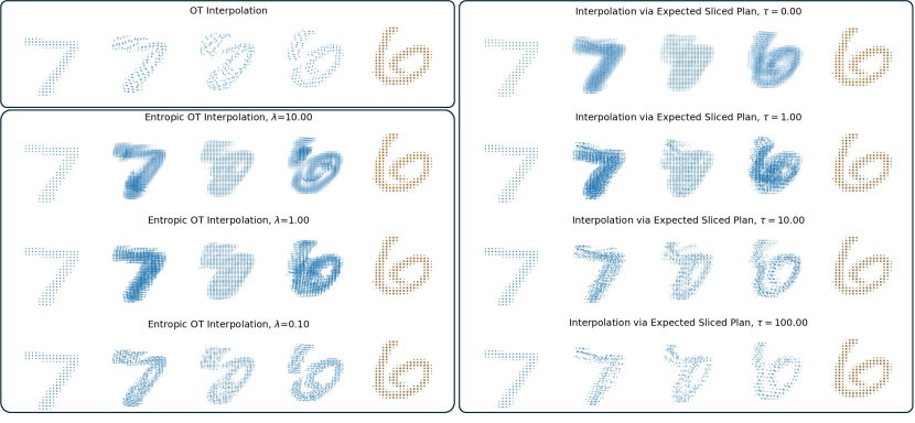
We use the Point Cloud MNIST 2D dataset (Garcia, 2023), a reimagined version of the classic MNIST dataset (LeCun, 1998), where each image is represented as a set of weighted 2D point clouds instead of pixel values. In Figure 4, we illustrate the interpolation between two point clouds that represent digits 7 and 6. Since the point clouds are discrete probability measures with non-uniform mass, we perform three different interpolation schemes via $((1-t)x+ty)_{\#}\gamma$ where $0\leq t\leq 1$ for different transportation plans $\gamma$ , namely:

1.

$\gamma=\gamma^{*}$ , an optimal transportation plan for $W_{2}(\cdot,\cdot)$ ;
2.

a transportation plan $\gamma$ obtained from solving an entropically regularized transportation problem (performed for three different regularization parameters $\lambda$ );
3.

$\gamma=\bar{\gamma}$ : the expected sliced transport plan computed using $\sigma_{\tau}$ given by formula (14) (or (15) for implementations) for four different values of the temperature parameter $\tau$ .

As the temperature increases, the transportation plan exhibits less mass splitting, similar to the effect of decreasing the regularization parameter $\lambda$ in entropic OT. However, unlike entropic OT, where smaller regularization parameters require more iterations for convergence, the computation time for expected sliced transport remains unaffected by changes in temperature.

3.4 Weak Convergence

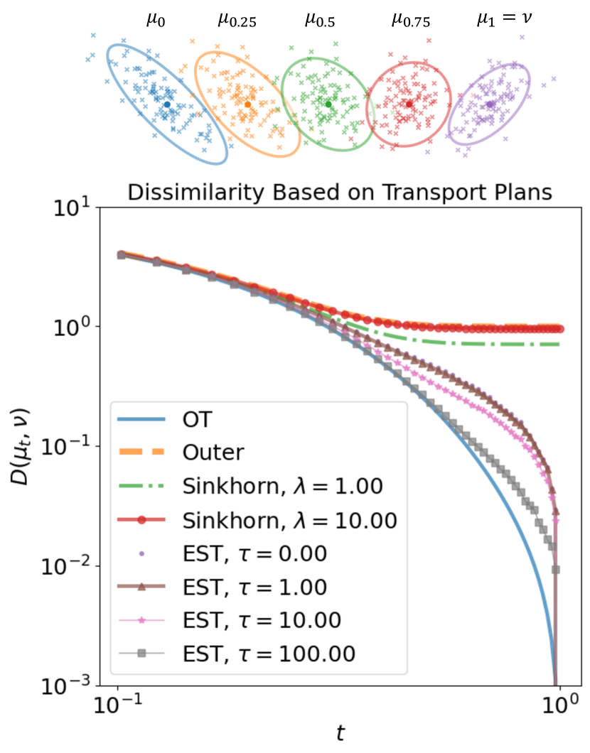
Given finite discrete probability measures $\mu$ and $\nu$ , we consider $\mu_{t}$ , for $0\leq t\leq 1$ , the Wasserstein geodesic between $\mu$ and $\nu$ . In particular, $\mu_{t}$ is a curve of probability measures that interpolates $\mu$ and $\nu$ , that is $\mu_{1}=\mu$ and $\mu_{1}=\nu$ . Moreover, we have that $W_{2}(\mu_{t},\nu)=(1-t)W_{2}(\mu,\nu)\longrightarrow 0$ as $t\to 1$ , or equivalently, we can say $\mu_{t}$ converges in the weak^∗-topology to $\nu$ . Figure 5 illustrates that the expected sliced distance also satisfies $\mathcal{D}_{2}(\mu_{t},\nu)\longrightarrow 0$ as $t\to 1$ . Indeed, this experimental conclusion is justified by the following theoretical result:

Let $\mu,\mu_{n}\in\mathcal{P}(\Omega)$ be discrete measures with finite or countable support, where $\Omega\subset\mathbb{R}^{d}$ is compact. Assume $\sigma\ll\mathcal{U}(\mathbb{S}^{d-1})$ . Then, $\mathcal{D}_{p}(\mu_{n},\mu)\to 0$ if and only if $\mu_{n}\stackrel{{\scriptstyle*}}{{\rightharpoonup}}\mu$ .

We present its proof in Appendix B.

For the experiment, $\mu$ and $\nu$ are chosen to be discrete measures with $N$ particles of uniform mass, sampled from two Gaussian distributions (see Figure 5, top). For different values of time, $0\leq t\leq 1$ , we compute different discrepancies, $\sum_{i=1}^{N}\sum_{j=1}^{N}\|x_{i}-y_{j}\|^{2}\gamma^{\mu_{t},\nu}_{ij}$ , calculated for various transport plans: (1) the optimal transport plan, (2) the outer product plan $\mu_{t}\otimes\nu$ , (3) the plan obtained from entropic OT with two different regularization parameters $\lambda$ , and (4) our proposed expected sliced plan computed with $\sigma_{\tau}$ given in (14) for four different temperature parameters $\tau$ . As $\mu_{t}$ converges to $\nu$ , it is evident that both the OT and our proposed EST distance approach zero, while the entropic OT and outer product plans, as expected, do not converge to zero.

3.5 Transport-Based Embedding

Following the linear optimal transportation (LOT) framework, also referred to as the Wasserstein or transport-based embedding framework (Wang et al., 2013; Kolouri et al., 2021; Nenna & Pass, 2023; Bai et al., 2023; Martín et al., 2024), we investigate the application of our proposed transportation plan in point cloud classification. Let $\mu_{0}=\sum_{i=1}^{N}\alpha_{i}\delta_{x_{i}}$ , denote a reference probability measure, and let $\mu_{k}=\sum_{j=1}^{N_{k}}\beta^{k}_{j}\delta_{y^{k}_{j}}$ denote a target probability measure. Let $\gamma^{\mu_{0},\mu_{k}}$ denote a transportation plan between $\mu_{0}$ and $\mu_{k}$ , and define the barycentric projection (Ambrosio et al., 2011, Definition 5.4.2) of this plan as:

b_{i}(\gamma^{\mu_{0},\mu_{k}}):=\frac{1}{\alpha_{i}}\sum_{j=1}^{N_{k}}\gamma^{\mu_{0},\mu_{k}}_{ij}y^{k}_{j},\qquad i\in{1,...,N}.

(16)

Note that $b_{i}(\gamma^{\mu_{0},\mu_{k}})$ represents the center of mass to which $x_{i}$ from the reference measure is transported according to the transportation plan $\gamma^{\mu_{0},\mu_{k}}$ . When $\gamma^{\mu_{0},\mu_{k}}$ is the OT plan, the LOT framework of Wang et al. (2013) uses

[\phi(\mu_{k})]_{i}:=b_{i}(\gamma^{\mu_{0},\mu_{k}})-x_{i},\qquad i\in{1,...,N}

as an embedding $\phi$ for the measure $\mu^{k}$ . This framework, as demonstrated in Kolouri et al. (2021), can be used to define a permutation-invariant embedding for sets of features and, more broadly, point clouds. More precisely, given a point cloud $\mathcal{Y}_{k}=\{(\beta_{j}^{k},y^{k}_{j})\}_{j=1}^{N_{k}}$ , where $\sum_{j=1}^{N_{k}}\beta_{j}^{k}=1$ and $\beta_{j}$ represent the mass at location $y_{j}$ , we represent this point cloud as a discrete measure $\mu_{k}$ .

In this section, we use a reference measure with $N$ particles of uniform mass to embed the digits from the Point Cloud MNIST 2D dataset using various transportation plans. We then perform a logistic regression on the embedded digits and present the results in Figure 6. The figure shows a 2D t-SNE visualization of the embedded point clouds using: (1) the OT plan, (2) the entropic OT plan with two different regularization parameters, and (3) our expected sliced plan with two temperature parameters (using $N=100$ for all methods). In addition, we report the test accuracy of these embeddings for different reference sizes.

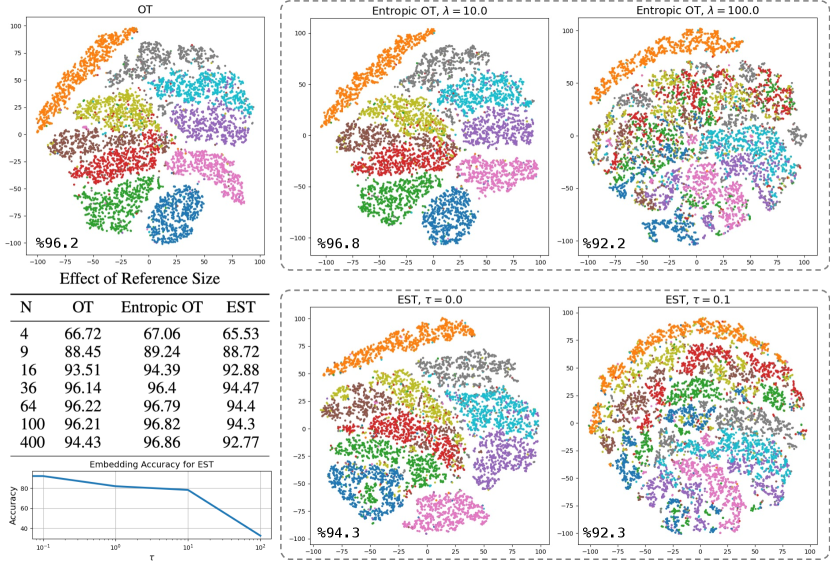
Lastly, we make an interesting observation about the embedding computed using EST. As we reduce the temperature, i.e., increase $\tau$ , the embedding becomes progressively less informative. We attribute this to the dependence of $\sigma_{\tau}$ on $\mu_{k}$ . In other words, the embedding is computed with respect to different $\sigma_{\tau}$ for different measures, leading to inaccuracies when comparing the embedded measures. This finding also suggests that the min-SWGG framework, while meritorious, may not be well-suited for defining a transport-based embedding.

4 Conclusions

In this paper, we explored the feasibility of constructing transportation plans between two probability measures using the computationally efficient sliced optimal transport (OT) framework. We introduced the Expected Sliced Transport (EST) framework and proved that it provides a valid metric for comparing discrete probability measures while preserving the computational efficiency of sliced transport and enabling explicit mass coupling. Through a diverse set of numerical experiments, we illustrated the behavior of this newly introduced transportation plan. Additionally, we demonstrated how the temperature parameter in our approach offers a flexible framework that connects our method to the recently proposed min-Sliced Wasserstein Generalized Geodesics (min-SWGG) framework. Finally, the theoretical insights and experimental results presented here open up new avenues for developing efficient transport-based algorithms in machine learning and beyond.

Acknowledgement

SK acknowledges support from NSF CAREER Award #2339898. MT was supported by the Leverhulme Trust Research through the Project Award “Robust Learning: Uncertainty Quantification, Sensitivity and Stability” (grant agreement RPG-2024-051) and the EPSRC Mathematical and Foundations of Artificial Intelligence Probabilistic AI Hub (grant agreement EP/Y028783/1).

References

Ambrosio et al. (2011) Luigi Ambrosio, Edoardo Mainini, and Sylvia Serfaty. Gradient flow of the chapman–rubinstein–schatzman model for signed vortices. In Annales de l’IHP Analyse non linéaire, volume 28, pp. 217–246, 2011.
Arjovsky et al. (2017) Martin Arjovsky, Soumith Chintala, and Léon Bottou. Wasserstein generative adversarial networks. In International conference on machine learning, pp. 214–223. PMLR, 2017.
Bai et al. (2023) Yikun Bai, Ivan Vladimir Medri, Rocio Diaz Martin, Rana Shahroz, and Soheil Kolouri. Linear optimal partial transport embedding. In International Conference on Machine Learning, pp. 1492–1520. PMLR, 2023.
Basu et al. (2014) Saurav Basu, Soheil Kolouri, and Gustavo K Rohde. Detecting and visualizing cell phenotype differences from microscopy images using transport-based morphometry. Proceedings of the National Academy of Sciences, 111(9):3448–3453, 2014.
Bunne et al. (2024) Charlotte Bunne, Geoffrey Schiebinger, Andreas Krause, Aviv Regev, and Marco Cuturi. Optimal transport for single-cell and spatial omics. Nature Reviews Methods Primers, 4(1):58, 2024.
Chapel et al. (2020) Laetitia Chapel, Mokhtar Z Alaya, and Gilles Gasso. Partial optimal tranport with applications on positive-unlabeled learning. Advances in Neural Information Processing Systems, 33:2903–2913, 2020.
Courty et al. (2014) Nicolas Courty, Rémi Flamary, and Devis Tuia. Domain adaptation with regularized optimal transport. In Machine Learning and Knowledge Discovery in Databases: European Conference, ECML PKDD 2014, Nancy, France, September 15-19, 2014. Proceedings, Part I 14, pp. 274–289. Springer, 2014.
Cuturi (2013) Marco Cuturi. Sinkhorn distances: Lightspeed computation of optimal transport. Advances in neural information processing systems, 26:2292–2300, 2013.
Feydy et al. (2019) Jean Feydy, Thibault Séjourné, François-Xavier Vialard, Shun-ichi Amari, Alain Trouvé, and Gabriel Peyré. Interpolating between optimal transport and mmd using sinkhorn divergences. In The 22nd International Conference on Artificial Intelligence and Statistics, pp. 2681–2690. PMLR, 2019.
Frogner et al. (2015) Charlie Frogner, Chiyuan Zhang, Hossein Mobahi, Mauricio Araya, and Tomaso A Poggio. Learning with a Wasserstein loss. Advances in neural information processing systems, 28, 2015.
Garcia (2023) Cristian Garcia. Point cloud mnist 2d dataset, 2023. URL https://www.kaggle.com/datasets/cristiangarcia/pointcloudmnist2d. Accessed: 2024-09-28.
Gretton et al. (2012) Arthur Gretton, Karsten M Borgwardt, Malte J Rasch, Bernhard Schölkopf, and Alexander Smola. A kernel two-sample test. The Journal of Machine Learning Research, 13(1):723–773, 2012.
Kolouri et al. (2017) Soheil Kolouri, Se Rim Park, Matthew Thorpe, Dejan Slepcev, and Gustavo K. Rohde. Optimal mass transport: Signal processing and machine-learning applications. IEEE Signal Processing Magazine, 34(4):43–59, 2017. 10.1109/MSP.2017.2695801.
Kolouri et al. (2021) Soheil Kolouri, Navid Naderializadeh, Gustavo K. Rohde, and Heiko Hoffmann. Wasserstein embedding for graph learning. In International Conference on Learning Representations, 2021. URL https://openreview.net/forum?id=AAes_3W-2z.
LeCun (1998) Yann LeCun. The mnist database of handwritten digits. http://yann. lecun. com/exdb/mnist/, 1998.
Maggi (2023) Francesco Maggi. Optimal mass transport on Euclidean spaces, volume 207. Cambridge University Press, 2023.
Mahey et al. (2023) Guillaume Mahey, Laetitia Chapel, Gilles Gasso, Clément Bonet, and Nicolas Courty. Fast optimal transport through sliced generalized wasserstein geodesics. In Thirty-seventh Conference on Neural Information Processing Systems, 2023. URL https://openreview.net/forum?id=n3XuYdvhNW.
Martín et al. (2024) Rocío Díaz Martín, Ivan V Medri, and Gustavo Kunde Rohde. Data representation with optimal transport. arXiv preprint arXiv:2406.15503, 2024.
Nadjahi et al. (2020) Kimia Nadjahi, Alain Durmus, Lénaïc Chizat, Soheil Kolouri, Shahin Shahrampour, and Umut Simsekli. Statistical and topological properties of sliced probability divergences. Advances in Neural Information Processing Systems, 33:20802–20812, 2020.
Nenna & Pass (2023) Luca Nenna and Brendan Pass. Transport type metrics on the space of probability measures involving singular base measures. Applied Mathematics & Optimization, 87(2):28, 2023.
Paty & Cuturi (2019) François-Pierre Paty and Marco Cuturi. Subspace robust wasserstein distances. In International conference on machine learning, pp. 5072–5081. PMLR, 2019.
Peyré & Cuturi (2019) Gabriel Peyré and Marco Cuturi. Computational optimal transport: With applications to data science. Foundations and Trends in Machine Learning, 11(5-6):355–607, 2019.
Rabin et al. (2011) Julien Rabin, Gabriel Peyré, Julie Delon, and Marc Bernot. Wasserstein barycenter and its application to texture mixing. In International Conference on Scale Space and Variational Methods in Computer Vision, pp. 435–446. Springer, 2011.
Rabin et al. (2014) Julien Rabin, Sira Ferradans, and Nicolas Papadakis. Adaptive color transfer with relaxed optimal transport. In 2014 IEEE international conference on image processing (ICIP), pp. 4852–4856. IEEE, 2014.
Rowland et al. (2019) Mark Rowland, Jiri Hron, Yunhao Tang, Krzysztof Choromanski, Tamas Sarlos, and Adrian Weller. Orthogonal estimation of wasserstein distances. In The 22nd International Conference on Artificial Intelligence and Statistics, pp. 186–195. PMLR, 2019.
Santambrogio (2015) Filippo Santambrogio. Optimal transport for applied mathematicians, volume 55. Birkäuser, NY, 2015.
Schmitzer (2016) Bernhard Schmitzer. A sparse multiscale algorithm for dense optimal transport. Journal of Mathematical Imaging and Vision, 56:238–259, 2016.
Villani (2009) Cedric Villani. Optimal transport: old and new. Springer, 2009. URL https://www.cedricvillani.org/sites/dev/files/old_images/2012/08/preprint-1.pdf.
Villani (2021) Cédric Villani. Topics in optimal transportation, volume 58. American Mathematical Soc., 2021.
Wang et al. (2013) Wei Wang, Dejan Slepčev, Saurav Basu, John A Ozolek, and Gustavo K Rohde. A linear optimal transportation framework for quantifying and visualizing variations in sets of images. International journal of computer vision, 101:254–269, 2013.

Appendix A Proof of Theorem 2.10: Metric property of the expected sliced discrepancy for discrete probability measures

A.1 Preliminaries on Expected Sliced Transportation

Remark A.1 (Figure 1).

Let us elaborate on explaining Figure 1. (a) Visualization for uniform discrete measures $\mu^{1}=\frac{1}{3}(\delta_{x_{1}}+\delta_{x_{2}}+\delta_{x_{3}})$ (green circles), $\mu^{2}=\frac{1}{3}(\delta_{y_{1}}+\delta_{y_{2}}+\delta_{y_{3}})$ (blue circles) in $\mathcal{P}_{(N)}(\mathbb{R}^{d})$ with $n=3$ . Given an angle $\theta$ (red unit vector), when sorting $\{\theta\cdot x_{i}\}_{i=1}^{3}$ and $\{\theta\cdot y_{j}\}_{j=1}^{3}$ we use permutations $\zeta_{\theta}$ and $\tau_{\theta}$ given by $\zeta_{\theta}(2)=1,\zeta_{\theta}(1)=2,\zeta_{\theta}(3)=3$ , and $\tau_{\theta}(1)=1$ , $\tau_{\theta}(3)=2$ , $\tau_{\theta}(2)=3$ . The optimal transport map between $\theta_{\#}\mu^{1}$ (green triangles) and $\theta_{\#}\mu^{2}$ (blue triangles) is given by the following assignment: $\theta\cdot x_{\zeta_{\theta}^{-1}(1)}=\theta\cdot x_{2}\longmapsto\theta\cdot y_{1}=\theta\cdot y_{\tau_{\theta}^{-1}(1)}$ , $\theta\cdot x_{\zeta_{\theta}^{-1}(2)}=\theta\cdot x_{1}\longmapsto\theta\cdot y_{3}=\theta\cdot y_{\tau_{\theta}^{-1}(2)}$ , $\theta\cdot x_{\zeta_{\theta}^{-1}(3)}=\theta\cdot x_{3}\longmapsto\theta\cdot y_{2}=\theta\cdot y_{\tau_{\theta}^{-1}(3)}$ . This gives rise to the plan $\Lambda_{\theta}^{\mu^{1},\mu^{2}}$ given in (7) with is represented by solid arrows in the first panel. The lifted plan $\gamma_{\theta}^{\mu^{1},\mu^{2}}$ defined in (8) is represented in the second panel by dashed assignments. (b) Visualization for finite discrete measures $\mu^{1}=0.1\delta_{x_{1}}+0.3\delta_{x_{2}}+0.6\delta_{x_{3}}$ (green circles), $\mu^{2}=0.5\delta_{y_{1}}+0.3\delta_{y_{2}}+0.2\delta_{y_{3}}$ (blue circles). When projection according a given direction $\theta$ , the locations with green masses $0.3$ and $0.6$ overlap, as well as the locations with blue masses $0.2$ and $0.3$ . Thus, the mass of $\theta_{\#}\mu^{1}$ is concentrated at two green points (triangles) on the line determined by $\theta$ , each one with $0.1$ and $0.9$ of the total mass, and similarly $\theta_{\#}\mu^{2}$ is concentrated at two points (blue triangles) each one with $0.5$ of the total mass.

Now, let us prove Lemma 2.3, that is, let us show that each measure $\gamma_{\theta}^{\mu^{1},\mu^{2}}$ defined in (9) is a transport plan in $\Gamma(\mu^{1},\mu^{2})$ .

Proof of Lemma 2.3.

Let $x\in\mathbb{R}^{d}$ . First, if $p(x)=0$ , then $u_{\theta}^{\mu^{1},\mu^{2}}(x,y)=0$ for every $y\in\mathbb{R}^{d}$ , and so $\gamma_{\theta}^{\mu^{1},\mu^{2}}(\{x\}\times\mathbb{R}^{d})=0=p(x)=\mu^{1}(\{x\})$ . Now, assume that $p(x)\not=0$ , then

	$\displaystyle\sum_{y\in\mathbb{R}^{d}}u_{\theta}^{\mu^{1},\mu^{2}}(x,y)$	$\displaystyle=\frac{p(x)}{P(\bar{x}^{\theta})}\sum_{y\in\mathbb{R}^{d}:\,q(y)\not=0}\frac{q(y)}{Q(\bar{y}^{\theta})}\Lambda_{\theta}^{\mu^{1},\mu^{2}}(\{(\bar{x}^{\theta},\bar{y}^{\theta})\})$
		$\displaystyle=\frac{p(x)}{P(\bar{x}^{\theta})}\sum_{\bar{y}^{\theta}\in\mathbb{R}^{d}/{\sim_{\theta}}:\,Q(\bar{y}^{\theta})\not=0}\left(\sum_{y\in\bar{y}^{\theta}}q(y)\right)\frac{1}{Q(\bar{y}^{\theta})}\Lambda_{\theta}^{\mu^{1},\mu^{2}}(\{(\bar{x}^{\theta},\bar{y}^{\theta})\})$
		$\displaystyle=\frac{p(x)}{P(\bar{x}^{\theta})}\sum_{\bar{y}^{\theta}\in\mathbb{R}^{d}/{\sim_{\theta}}:\,Q(\bar{y}^{\theta})\not=0}Q(\bar{y}^{\theta})\frac{1}{Q(\bar{y}^{\theta})}\Lambda_{\theta}^{\mu^{1},\mu^{2}}(\{(\bar{x}^{\theta},\bar{y}^{\theta})\})$
		$\displaystyle=\frac{p(x)}{P(\bar{x}^{\theta})}\sum_{\bar{y}^{\theta}\in\mathbb{R}^{d}/{\sim_{\theta}}}\Lambda_{\theta}^{\mu^{1},\mu^{2}}(\{(\bar{x}^{\theta},\bar{y}^{\theta})\})=\frac{p(x)}{P(\bar{x}^{\theta})}P(\bar{x}^{\theta})=p(x).$

Thus, $\gamma_{\theta}^{\mu^{1},\mu^{2}}(\{x\}\times\mathbb{R}^{d})=p(x)=\mu^{1}(\{x\})$ for every $x\in\mathbb{R}^{d}$ . Similarly, $\sum_{x\in\mathbb{R}^{d}}u_{\theta}^{\mu^{1},\mu^{2}}(x,y)=q(y)$ , or equivalently, $\gamma_{\theta}^{\mu^{1},\mu^{2}}(\mathbb{R}^{d}\times\{y\})=q(x)=\mu^{2}(\{y\})$ for every $y\in\mathbb{R}^{d}$ . ∎

Remark A.2 (Expected Sliced Transport for uniform discrete measures).

Let $\mu^{1},\mu^{2}\in\mathcal{P}_{(N)}(\mathbb{R}^{d})$ of the form $\mu^{1}=\frac{1}{N}\sum_{i=1}^{N}\delta_{x_{i}}$ , $\mu^{2}=\frac{1}{N}\sum_{j=1}^{N}\delta_{y_{j}}$ . Then, the expected sliced transport plan between $\mu^{1}$ and $\mu^{2}$ , $\bar{\gamma}^{\mu^{1},\mu^{2}}=\mathbb{E}_{\theta\sim\sigma}[\gamma_{\theta}^{\mu^{1},\mu^{2}}]$ , defines a discrete measure on $\mathcal{P}(\mathbb{R}^{d}\times\mathbb{R}^{d})$ supported on $\{(x_{i},y_{j})\}_{i,j\in[N]}$ where it takes the values

\bar{\gamma}^{\mu^{1},\mu^{2}}(\{x_{i},y_{j}\})=\int_{\mathbb{S}^{d-1}}\gamma_{\theta}^{\mu^{1},\mu^{2}}(\{x_{i},y_{j}\})d\sigma(\theta)\qquad\forall i\in[N],j\in[N].

(17)

Thus, it can be regarded as an $N\times N$ matrix whose $(i,j)$ -entry is given by (17). Moreover, each $N\times N$ matrix $u_{\theta}^{\mu^{1},\mu^{2}}$ defined by (6) can be obtained by swapping rows from the $N\times N$ identity matrix multiplied by $1/N$ , there are finitely many matrices (precisely, $N!$ matrices in total). Hence, the function $\theta\mapsto u_{\theta}^{\mu^{1},\mu^{2}}$ is a piece-wise constant matrix-valued function. Thus, the function $\theta\mapsto\gamma_{\theta}^{\mu^{1},\mu^{2}}$ (where $\gamma_{\theta}^{\mu^{1},\mu^{2}}$ is an in (8)) is a measurable function. This can be generalized for any pair of finite discrete measures as in the following remarks.

Remark A.3 (Expected Sliced Transport for finite discrete measures).

Consider arbitrary finite discrete measures $\mu^{1}=\sum_{i=1}^{n}p(x_{i})\delta_{x_{i}}$ and $\mu^{2}=\sum_{j=1}^{m}q(y_{i})\delta_{y_{j}}$ , i.e., discrete measures with finite support.

•

Fix $x_{i},y_{j}\in\mathbb{R}^{d}$ , then $\theta\mapsto\frac{p(x_{i})q(y_{j})}{P(\bar{x}_{i}^{\theta})Q(\bar{y}_{j}^{\theta})}\not=1$ for all but a finite number of directions. This is due to the fact that only for finitely many directions $\theta$ we obtain overlaps of the projected points $\theta\cdot x$ .
•

The optimal transport plan $\Lambda_{\theta}^{\mu^{1},\mu^{2}}$ is given by “matching from left to right until fulfilling the target bins”: that is, one has to order the points similarly as in (3) and consider an “increasing” assignment plan. Since the order of $\{\theta\cdot x_{i}\}_{i=1}^{n}$ and $\{\theta\cdot y_{j}\}_{j=1}^{m}$ changes a finite number of times when varying $\theta\in\mathbb{S}^{d-1}$ , the function $\theta\mapsto\Lambda_{\theta}^{\mu^{1},\mu^{2}}$ takes a finite number of possible transportation plan options.

Thus, the range of $\theta\mapsto u_{\theta}^{\mu^{1},\mu^{2}}$ is finite.

Remark A.4 ( $\bar{\gamma}^{\mu^{1},\mu^{2}}$ is well-defined for finite discrete measures).

First, we notice that for each $\theta$ , the support of $\Lambda_{\theta}^{\mu^{1},\mu^{2}}$ is finite or countable, and so the support of $\gamma_{\theta}^{\mu^{1},\mu^{2}}$ is also finite or countable. Given an arbitrary point $(x,y)\in\mathbb{R}^{d}\times\mathbb{R}^{d}$ , we have to justify that the function $\mathbb{S}^{d-1}\ni\theta\mapsto u_{\theta}^{\mu^{1},\mu^{2}}(x,y)$ is (Borel)-measurable: If the supports of $\mu^{1}$ and $\mu^{2}$ are finite, by Remark A.3, $\theta\mapsto u_{\theta}^{\mu^{1},\mu^{2}}$ is a piece-wise constant function, and so it is measurable and integrable on the sphere. For the general case, when the supports of $\mu^{1}$ and $\mu^{2}$ are countable, we refer to Remark A.14.

Lemma A.5 ( $\bar{\gamma}^{\mu^{1},\mu^{2}}$ is a transportation plan between $\mu^{1}$ and $\mu^{2}$ ).

We have that $\bar{\gamma}^{\mu^{1},\mu^{2}}\in\Gamma(\mu^{1},\mu^{2})$ , i.e., it has marginals $\mu^{1}$ and $\mu^{2}$ . This is because for each $\theta\in\mathbb{S}^{d-1}$ , $\gamma_{\theta}^{\mu^{1},\mu^{2}}\in\Gamma(\mu^{1},\mu^{2})$ and because $\sigma$ is a probability measure on $\mathbb{S}^{d-1}$ . Then, $\bar{\gamma}^{\mu^{1},\mu^{2}}$ is a convex combination of transport plans $\gamma_{\theta}^{\mu^{1},\mu^{2}}$ , and since $\Gamma(\mu^{1},\mu^{2})$ is a convex set, we obtain that $\bar{\gamma}^{\mu^{1},\mu^{2}}\in\Gamma(\mu^{1},\mu^{2})$ . Precisely, for every test function $\phi:\mathbb{R}^{d}\to\mathbb{R}$

	$\displaystyle\int_{\mathbb{R}^{d}\times\mathbb{R}^{d}}\phi(x)d\bar{\gamma}^{\mu^{1},\mu^{2}}(x,y)$	$\displaystyle=\int_{\mathbb{S}^{d-1}}\int_{\mathbb{R}^{d}\times\mathbb{R}^{d}}\phi(x)d\gamma_{\theta}^{\mu^{1},\mu^{2}}(x,y)d\sigma(\theta)$
		$\displaystyle=\int_{\mathbb{S}^{d-1}}\int_{\mathbb{R}^{d}}\phi(x)d\mu^{1}(x)d\sigma(\theta)=\int_{\mathbb{R}^{d}}\phi(x)d\mu^{1}(x)$

Similarly, $\int_{\mathbb{R}^{d}\times\mathbb{R}^{d}}\psi(y)d\bar{\gamma}^{\mu^{1},\mu^{2}}(x,y)=\int_{\mathbb{R}^{d}}\psi(y)d\mu^{2}(y),$ and so $\bar{\gamma}^{\mu^{1},\mu^{2}}$ has marginals $\mu^{1}$ and $\mu^{2}$ .

A.2 An auxiliary result

For simplicity, in this paper we consider the strictly convex cost $\|x-y\|^{p}$ ( $1<p<\infty$ ). Also, in this section we consider $\sigma=\mathcal{U}(\mathbb{S}^{d-1})$ and in this case we denote $d\sigma(\theta)=d\theta$ .

Proposition A.6.

Let $\Omega\subset\mathbb{R}^{d}$ be a compact set, and let $\mu^{1},\mu^{2}\in\mathcal{P}(\Omega)$ . Let $(\mu_{n}^{1})_{n\in\mathbb{N}},(\mu_{n}^{2})_{n\in\mathbb{N}}\subset\mathcal{P}(\Omega)$ be sequences such that, for $i=1,2$ , $\mu_{n}^{i}\rightharpoonup^{*}\mu^{i}$ as $n\to\infty$ , where the limit is in the weak*-topology. For each $n\in\mathbb{N}$ , consider optimal transportation plans $\gamma_{n}\in\Gamma^{*}(\mu^{1}_{n},\mu^{2}_{n})$ . Then, there exists a subsequence such that $\gamma_{n_{k}}\rightharpoonup^{*}\gamma$ , for some optimal transportation plan $\gamma\in\Gamma^{*}(\mu^{1},\mu^{2})$ .

Proof.

As $(\gamma_{n})_{n\in\mathbb{N}}$ is a sequence of probability measures, their mass is 1, by Banach-Alaoglu Theorem, there exists a subsequence such that $\gamma_{n_{k}}\rightharpoonup^{*}\gamma$ , for some $\gamma\in\mathcal{P}(\Omega\times\Omega)$ . It is easy to see that the limit $\gamma$ has marginals $\mu^{1},\mu^{2}$ . Indeed, given any test functions $\phi,\psi\in C(\Omega)$ , since each $\gamma_{n}$ has marginals $\mu_{n}^{1},\mu_{n}^{2}$ , we have

\displaystyle\int_{\Omega\times\Omega}\phi(x)d\gamma_{n}(x,y)=\int_{\Omega}\phi(x)d\mu_{n}^{1}(x)\quad\text{ and }\quad\int_{\Omega\times\Omega}\psi(y)d\gamma_{n}(x,y)=\int_{\Omega}\psi(y)d\mu_{n}^{2}(y)

and taking limit as $n\to\infty$ , we obtain

\displaystyle\int_{\Omega\times\Omega}\phi(x)d\gamma(x,y)=\int_{\Omega}\phi(x)d\mu^{1}(x)\quad\text{ and }\quad\int_{\Omega\times\Omega}\psi(y)d\gamma(x,y)=\int_{\Omega}\psi(y)d\mu^{2}(y).

Now, we only have to prove the optimality of $\gamma$ for the OT problem between $\mu^{1}$ and $\mu^{2}$ . Since $(x,y)\mapsto\|x-y\|^{p}$ is continuous and $\gamma_{n}$ , $\gamma$ are compactly supported, by using that for each $n\in\mathbb{N}$ , $\gamma_{n}$ is optimal for the OT problem between $\mu^{1}_{n}$ and $\mu^{2}_{n}$ , we have

	$\displaystyle\lim_{n\to\infty}\left(W_{p}(\mu^{1}_{n},\mu^{2}_{n})\right)^{p}$	$\displaystyle=\lim_{n\to\infty}\int_{\Omega\times\Omega}\\|x-y\\|^{p}d\gamma_{n}(x,y)\qquad$
		$\displaystyle=\int_{\Omega\times\Omega}\\|x-y\\|^{p}d\gamma(x,y)\geq\left(W_{p}(\mu^{1},\mu^{2})\right)^{p}$		(18)

Also, by hypothesis and (Santambrogio, 2015, Theorem 5.10) we have that for any $\nu\in\mathcal{P}(\Omega)$ ,

\lim_{n\to\infty}W_{p}(\mu_{n}^{1},\nu)=W_{p}(\mu^{1},\nu)\qquad\text{ and }\qquad\lim_{n\to\infty}W_{p}(\nu,\mu_{n}^{2})=W_{p}(\nu,\mu^{2}).

So, by using the the triangle inequality for the $p$ -Wasserstein distance we get

	$\displaystyle\lim_{n\to\infty}W_{p}(\mu^{1}_{n},\mu_{n}^{2})$	$\displaystyle\leq\lim_{n\to\infty}W_{p}(\mu^{1}_{n},\mu^{1})+\lim_{n\to\infty}W_{p}(\mu^{2},\mu_{n}^{2})+W_{p}(\mu^{1},\mu^{2})$
		$\displaystyle=0+W_{p}(\mu^{1},\mu^{2})=W_{p}(\mu^{1},\mu^{2})$		(19)

Therefore, from (19) and (18) we have that

\lim_{n\to\infty}W_{p}(\mu_{n}^{1},\mu^{2}_{n})=W_{p}(\mu^{1},\mu^{2}).

In particular, in (18) we have that the following equality holds:

\int_{\Omega\times\Omega}\|x-y\|^{p}d\gamma(x,y)=\left(W_{p}(\mu^{1},\mu^{2})\right)^{p}.

As a result, $\gamma$ is optimal for the OT problem between $\mu^{1}$ and $\mu^{2}$ . ∎

A.3 Finite discrete measures with rational weights

Let us denote by $\mathcal{P}_{\mathbb{Q}}(\mathbb{R}^{d})$ the set of finite discrete probability measures in $\mathbb{R}^{d}$ with rational weights, that is, $\mu\in\mathcal{P}_{\mathbb{Q}}(\mathbb{R}^{d})$ if and only if it is of the form $\mu=\sum_{i=1}^{m}q_{i}\delta_{x_{i}}$ with $x_{i}\in\mathbb{R}^{d}$ , $q_{i}\in\mathbb{Q}$ $\forall i\in[m]$ for some $m\in\mathbb{N}$ , and $\sum_{i=1}^{m}q_{i}=1$ . We have

\mathcal{P}_{(N)}(\mathbb{R}^{d})\subset\mathcal{P}_{\mathbb{Q}}(\mathbb{R}^{d}),\qquad\forall N\in\mathbb{N}.

In the definition of an uniform discrete measure $\mu=\frac{1}{N}\sum_{i=1}^{N}\delta_{x_{i}}\in\mathcal{P}_{(N)}(\mathbb{R}^{d})$ one can allow $x_{i}=x_{j}$ for some pairs of indexes $i\not=j$ .

Proposition A.7.

$\mathcal{D}_{p}(\cdot,\cdot)$ defined by (11) is a metric in $\mathcal{P}_{\mathbb{Q}}(\mathbb{R}^{d})$ .

Proof.

This was essentially pointed out Remark 2.9: When restricting to the space $\mathcal{P}_{(N)}(\mathbb{R}^{d})$ , our $\mathcal{D}_{p}(\cdot,\cdot)$ and the Projected Wasserstein distance presented in (Rowland et al., 2019) coincide. Rowland et al. (2019) prove the metric property. We recall here their main argument, which is used for showing the triangle inequality. Given $\mu^{1},\mu^{2},\mu^{3}\in\mathcal{P}_{(N)}(\mathbb{R}^{d})$ of the form $\mu^{1}=\frac{1}{N}\sum_{i=1}^{N}\delta_{x_{i}}$ , $\mu^{2}=\frac{1}{N}\sum_{i=1}^{N}\delta_{y_{i}}$ , $\mu^{3}=\frac{1}{N}\sum_{i=1}^{N}\delta_{z_{i}}$ . Fix $\theta\in\mathbb{S}^{d-1}$ , and consider permutations $\zeta_{\theta},\tau_{\theta},\xi_{\theta}\in\mathbf{S}_{N}$ , so that

	$\displaystyle\theta\cdot x_{\zeta_{\theta}^{-1}(1)}\leq\dots\leq\theta\cdot x_{\zeta_{\theta}^{-1}(N)},$
	$\displaystyle\theta\cdot y_{\tau_{\theta}^{-1}(1)}\leq\dots\leq\theta\cdot y_{\tau_{\theta}^{-1}(N)},$
	$\displaystyle\theta\cdot z_{\xi_{\theta}^{-1}(1)}\leq\dots\leq\theta\cdot z_{\xi_{\theta}^{-1}(N)}$

Thus, the key idea is that

	$\displaystyle\mathcal{D}_{p}(\mu^{1},\mu^{2})^{p}$	$\displaystyle=\int_{\mathbb{S}^{d-1}}\frac{1}{N}\sum_{i=1}^{N}\\|x_{\zeta_{\theta}^{-1}(i)}-y_{\tau_{\theta}^{-1}(i)}\\|^{p}d\theta=\sum_{\zeta,\tau,\xi\in\mathbf{S}_{N}}\frac{\mathbf{q}(\zeta,\tau,\xi)}{N}\sum_{i=1}^{N}\\|x_{\zeta^{-1}(i)}-y_{\tau^{-1}(i)}\\|^{p}$
	$\displaystyle\mathcal{D}_{p}(\mu^{2},\mu^{3})^{p}$	$\displaystyle=\int_{\mathbb{S}^{d-1}}\frac{1}{N}\sum_{i=1}^{N}\\|y_{\tau_{\theta}^{-1}(i)}-z_{\xi_{\theta}^{-1}(i)}\\|^{p}d\theta=\sum_{\zeta,\tau,\xi\in\mathbf{S}_{N}}\frac{\mathbf{q}(\zeta,\tau,\xi)}{N}\sum_{i=1}^{N}\\|y_{\tau^{-1}(i)}-z_{\xi^{-1}(i)}\\|^{p}$
	$\displaystyle\mathcal{D}_{p}(\mu^{3},\mu^{1})^{p}$	$\displaystyle=\int_{\mathbb{S}^{d-1}}\frac{1}{N}\sum_{i=1}^{N}\\|z_{\xi_{\theta}^{-1}(i)}-x_{\zeta_{\theta}^{-1}(i)}\\|^{p}d\theta=\sum_{\zeta,\tau,\xi\in\mathbf{S}_{N}}\frac{\mathbf{q}(\zeta,\tau,\xi)}{N}\sum_{i=1}^{N}\\|z_{\xi^{-1}(i)}-x_{\zeta^{-1}(i)}\\|^{p}$

where $\mathbf{q}\in\mathcal{P}(\mathbf{S}_{N}\times\mathbf{S}_{N}\times\mathbf{S}_{N})$ is such that $\mathbf{q}(\zeta,\tau,\xi)$ is the probability that the tuple permutations $(\zeta,\tau,\xi)=(\zeta_{\theta},\tau_{\theta},\xi_{\theta})$ are required, given that $\theta$ is drawn from $\mathrm{Unif}(\mathbb{S}^{d-1})$ . With these alternative expressions established by the authors in (Rowland et al., 2019), the triangle inequality follows from the standard Minkowski inequality for weighted finite $L^{p}$ -spaces.

Finally, notice that we have used the fact that each $\mu^{1}$ is associated to $N$ -indexes $\{1,\dots,N\}$ , without asking that the points $\{x_{i}\}$ do not overlap, i.e., they could be repeated. That is, given $\mu^{1}=\frac{1}{N}\sum_{i=1}^{n}\delta_{x_{i}}\in\mathcal{P}_{(N)}(\mathbb{R}^{d})$ one can allow $x_{i}=x_{j}$ for some pairs of indexes $i\not=j$ (analogously for $\mu^{2}$ and $\mu^{3}$ ). Thus, the proof also holds for measures in $\mathcal{P}_{\mathbb{Q}}(\mathbb{R}^{d})$ : Indeed, let $\mu^{1},\mu^{2},\mu^{3}\in\mathcal{P}_{\mathbb{Q}}(\mathbb{R}^{d})$ be of the form $\mu^{1}=\sum_{i=1}^{n_{1}}\frac{r_{i}^{1}}{s_{i}^{1}}\delta_{x_{i}}$ , $\mu^{2}=\sum_{i=1}^{n_{2}}\frac{r_{i}^{2}}{s_{i}^{2}}\delta_{y_{i}}$ , $\mu^{3}=\sum_{i=1}^{n_{3}}\frac{r_{i}^{3}}{s_{i}^{3}}\delta_{z_{i}}$ with $r_{i}^{j},q_{i}^{j}\in\mathbb{N}$ . First, consider the $n_{1}^{\prime}$ as the least common multiple of $\{s^{1}_{1},\dots,s_{n_{1}}^{1}\}$ and, for each $i\in[n_{1}]$ , let $\tilde{r}_{i}^{1}$ so that $\frac{\tilde{r}_{i}^{1}}{n_{1}^{\prime}}=\frac{r_{i}^{1}}{s_{i}^{1}}$ . Thus, we can rewrite $\mu^{1}=\sum_{i=1}^{n_{1}}\frac{\tilde{r}_{i}^{1}}{n_{1}^{\prime}}\delta_{x_{i}}$ . Notice that, since $\mu^{1}$ is a probability measure, we have $n_{1}^{\prime}=\sum_{i=1}^{n_{1}}{\tilde{r}_{i}^{1}}$ . Now, for each $i\in[n_{1}]$ such that $\tilde{r}_{i}^{1}>1$ , consider $\tilde{r}_{i}^{1}$ copies of the corresponding point $x_{i}$ so that we can rewrite $\mu^{1}=\sum_{i=1}^{n_{1}^{\prime}}\frac{1}{n_{1}^{\prime}}\delta_{x_{i}}$ (where we recall that $n_{1}^{\prime}=\sum_{i=1}^{n_{1}}{\tilde{r}_{i}^{1}}$ and the points $x_{i}$ in the new expression can be repeated, i.e., they are not necessarily all different). Repeat this process to rewrite $\mu^{2}=\sum_{i=1}^{n_{2}^{\prime}}\frac{1}{n_{2}^{\prime}}\delta_{y_{i}}$ , $\mu^{3}=\sum_{i=1}^{n_{3}^{\prime}}\frac{1}{n_{3}^{\prime}}\delta_{z_{i}}$ . Now, consider $N$ as the least common multiple of $n_{1}^{\prime},n_{2}^{\prime},n_{3}^{\prime}$ , and rewrite the measures as $\mu^{1}=\frac{1}{N}\sum_{i=1}^{N}\delta_{x_{i}}$ , $\mu^{2}=\frac{1}{N}\sum_{i=1}^{N}\delta_{y_{i}}$ , $\mu^{3}=\frac{1}{N}\sum_{i=1}^{N}\delta_{z_{i}}$ where the points $x_{i}$ , $y_{i}$ , $z_{i}$ can be repeated if needed. Thus, $\mu^{1},\mu^{2},\mu^{3}$ can be regarded as measures in $\mathcal{P}_{(N)}(\mathbb{R}^{d})$ where $\mathcal{D}_{p}(\cdot,\cdot)$ behaves as a metric. ∎

A.4 The proof for general finite discrete measures

We first introduce some notation. Consider a finite discrete probability measure $\mu\in\mathcal{P}(\mathbb{R}^{d})$ of the form $\mu=\sum_{i=1}^{m}p^{i}\delta_{x_{i}}$ , with general weights $p^{i}\in\mathbb{R}_{+}$ such that $\sum_{i=1}^{m}p^{i}=1$ . For each $i\in\{1,\dots,m-1\}$ , consider an increasing sequence of rational numbers $(p_{n}^{i})_{n\in\mathbb{N}}\subset\mathbb{Q}$ , with $0\leq p_{n}^{i}\leq p^{i}$ , such that $\lim_{n\to\infty}p^{i}_{n}=p^{i}$ . For $i=m$ , consider the sequence $(p_{n}^{m})_{n\in\mathbb{N}}\subset\mathbb{Q}$ defined by $0\leq p_{n}^{m}:=1-\sum_{i=1}^{m-1}p_{n}^{i}\leq 1$ . Thus, $\lim_{n\to\infty}p_{n}^{m}=1-\lim_{n\to\infty}\sum_{i=1}^{m-1}p_{n}^{i}=1-\sum_{i=1}^{m-1}p^{i}=p^{m}$ . Define the sequence of probability measures $(\mu_{n})_{n\in\mathbb{N}}$ given by $\mu_{n}:=\sum_{i=1}^{m}p^{i}_{n}\delta_{x_{i}}\in\mathcal{P}_{\mathbb{Q}}(\mathbb{R}^{d})$ . It is easy to show that $(\mu_{n})_{n\in\mathbb{N}}$ converges to $\mu$ in Total Variation (i.e., uniform convergence or strong convergence): Indeed, let $\varepsilon>0$ . For each $i\in[m]$ , let $N_{i}\in\mathbb{N}$ such that $|p^{i}_{n}-p^{i}|<\varepsilon/m$ $\forall n\geq N_{i}$ and define $N=\max\{N_{1},\dots,N_{m}\}$ . Now, given any set $B\subset\mathbb{R}^{d}$ we obtain, for $n\geq N$ ,

	$\displaystyle\|\mu_{n}(B)-\mu(B)\|$	$\displaystyle=\left\|\sum_{i\in[m]:\,x_{i}\in B}(p_{n}^{i}-p^{i})\right\|\qquad\text{($\mu_{n}$ and $\mu$ have the same support)}$
		$\displaystyle\leq\sum_{i\in[m]:\,x_{i}\in B}\|p_{n}^{i}-p^{i}\|\qquad\text{(triangle inequality)}$
		$\displaystyle\leq\sum_{i\in[m]}\|p_{n}^{i}-p^{i}\|\qquad\text{(sum over all indexes to get independence of the set $B$)}$
		$\displaystyle<\varepsilon.$

This shows that $\lim_{n\to\infty}\|\mu_{n}-\mu\|_{\mathrm{TV}}=0$ . Moreover, this shows that in this case, i.e., when approximating a finite discrete measure $\mu$ by a sequence of measures having the same support as $\mu$ , we only care about point-wise convergence.

We will now introduce some lemmas which together with the above proposition will allow us to prove the metric property of $\mathcal{D}_{p}(\cdot,\cdot)$ for finite discrete probability measures. For all of them we will consider:

•

$\mu^{1},\mu^{2}$ two finite discrete probability measures in $\mathbb{R}^{d}$ given by $\mu^{1}=\sum_{i=1}^{m_{1}}p^{i}\delta_{x_{i}}$ , $\mu^{2}=\sum_{j=1}^{m_{2}}q^{j}\delta_{y_{j}}$
•

$(\mu^{1}_{n})_{n\in\mathbb{N}}$ , $(\mu^{2}_{n})_{n\in\mathbb{N}}$ approximating sequences of probability measures $\mu^{1}_{n}=\sum_{i=1}^{m_{1}}p^{i}_{n}\delta_{x_{i}}$ , $\mu^{2}_{n}=\sum_{j=1}^{m_{2}}q^{j}_{n}\delta_{y_{j}}$ , with rational weights $\{p^{i}_{n}\}$ , $\{q^{j}_{n}\}$ , defined in analogy to what we have already done, i.e., so that, for $k=1,2$ we have that $(\mu^{k}_{n})_{n\in\mathbb{N}}$ is a sequence of probability measures that converges to $\mu^{k}$ in Total Variation).

Also, for each $\theta$ , $\Lambda_{\theta}^{\mu^{1},\mu^{2}}$ denotes the unique optimal transport plan between $\theta_{\#}\mu^{1}$ and $\theta_{\#}\mu^{2}$ ; $\gamma_{\theta}^{\mu^{1},\mu^{2}}$ denotes lifted transport plan between $\mu^{1}$ and $\mu^{2}$ given as in (9); and $\bar{\gamma}^{\mu^{1},\mu^{2}}$ the expected sliced transport plan between $\mu^{1}$ and $\mu^{2}$ given as in (10). Similarly, for each $n\in\mathbb{N}$ we consider the plans $\Lambda_{\theta}^{\mu^{1}_{n},\mu^{2}_{n}}$ , $\gamma_{\theta}^{{\mu^{1}_{n},\mu^{2}_{n}}}$ , and $\bar{\gamma}^{{\mu^{1}_{n},\mu^{2}_{n}}}$ .

Lemma A.8.

The sequence $\left(\Lambda_{\theta}^{\mu^{1}_{n},\mu_{n}^{2}}\right)_{n\in\mathbb{N}}$ converges to $\Lambda_{\theta}^{\mu^{1},\mu^{2}}$ in Total Variation.

Lemma A.9.

The sequence $\left(\gamma_{\theta}^{\mu^{1}_{n},\mu_{n}^{2}}\right)_{n\in\mathbb{N}}$ converges to $\gamma_{\theta}^{\mu^{1},\mu^{2}}$ in Total Variation.

Lemma A.10.

The sequence $\left(\bar{\gamma}^{\mu_{n}^{1},\mu_{n}^{2}}\right)_{n\in\mathbb{N}}$ converges to $\bar{\gamma}^{\mu^{1},\mu^{2}}$ in Total Variation.

Lemma A.11.

$\displaystyle\lim_{n\to\infty}\mathcal{D}_{p}(\mu^{1}_{n},\mu^{2}_{n})=\mathcal{D}_{p}(\mu^{1},\mu^{2})$ .

In general, notice that since for every $i\in[m_{1}]$ , $j\in[m_{2}]$ we have that $\lim_{n\to\infty}p_{n}^{i}=p^{i}$ , and $\lim_{n\to\infty}q_{n}^{j}=p^{j}$ , then we obtain that $\lim_{n\to\infty}P_{n}^{i}=P^{i}$ , and $\lim_{n\to\infty}Q_{n}^{j}=Q^{j}$ , where $P^{i}=\sum_{i\in[m_{1}]:x_{i}\in\bar{x}_{i}^{\theta}}p^{i}$ , $Q^{j}=\sum_{j\in[m_{2}]:y_{j}\in\bar{y}_{j}^{\theta}}q^{j}$ , and where, for each $n\in\mathbb{N}$ , $P_{n}^{i}$ and $Q_{n}^{j}$ are analogously defined (see Subsection 2.2.2). Thus,

\lim_{n\to\infty}\frac{p^{i}_{n}q^{j}_{n}}{P^{i}_{n}Q^{j}_{n}}=\frac{p^{i}q^{j}}{P^{i}Q^{j}}\qquad\forall i\in[m_{1}],j\in[m_{2}].

(20)

Proof of Lemma A.8.

The support of all the measures we are considering are finite and so, the measures have compact support. Hence, we can apply Proposition A.6 to $\theta_{\#}\mu^{i}$ , $(\theta_{\#}\mu^{i})_{n\in\mathbb{N}}$ , $i=1,2$ . Specifically, given $(\Lambda_{\theta}^{\mu^{1}_{n},\mu^{2}_{n}})_{n\in\mathbb{N}}\in\Gamma^{*}(\theta_{\#}\mu_{n}^{1},\theta_{\#}\mu_{n}^{2})$ , there exists a subsequence $(\Lambda_{\theta}^{\mu^{1}_{n_{k}},\mu^{2}_{n_{k}}})_{K\in\mathbb{N}}$ and $\Lambda_{\theta}\in\Gamma^{*}(\theta_{\#}\mu^{1},\theta_{\#}\mu^{2})$ such that

\Lambda_{\theta}^{\mu^{1}_{n_{k}},\mu^{2}_{n_{k}}}\rightharpoonup^{*}\Lambda_{\theta}.

(21)

As we are in one dimension, the set $\Gamma^{*}(\theta_{\#}\mu^{1},\theta_{\#}\mu^{2})$ is a singleton, and so we have that $\Lambda_{\theta}=\Lambda_{\theta}^{\mu^{1},\mu^{2}}$ is the unique optimal transport plan. Since the supports of all the measures are the same, (that is, $\{(\theta\cdot x_{i},\theta\cdot y_{j})\}_{i\in[m_{1}],j\in[m_{2}]}$ ), the weak^∗ convergence in (21) implies the stronger convergence in Total Variation.

Now, suppose that the original sequence $(\Lambda_{\theta}^{\mu^{1}_{n},\mu^{2}_{n}})_{n\in\mathbb{N}}$ does not converge to $\Lambda_{\theta}^{\mu^{1},\mu^{2}}$ (in Total Variation). Then, given $\varepsilon>0$ , there exists a subsequence $(\Lambda_{\theta}^{\mu^{1}_{n_{j}},\mu^{2}_{n_{j}}})_{j\in\mathbb{N}}$ such that

\|\Lambda_{\theta}^{\mu^{1}_{n_{j}},\mu^{2}_{n_{j}}}-\Lambda_{\theta}^{\mu^{1},\mu^{2}}\|_{\mathrm{TV}}>\varepsilon

(22)

But again, from Proposition A.6, using that the supports of all the measures involved are the same set $\{(\theta\cdot x_{i},\theta\cdot y_{j})\}_{i\in[m_{1}],j\in[m_{2}]}$ , and the fact that $\Gamma^{*}(\theta_{\#}\mu^{1},\theta_{\#}\mu^{2})=\{\Lambda_{\theta}^{\mu^{1},\mu^{2}}\}$ (only one optimal transport plan), we have that there exists a sub-subsequence such that

\|\Lambda_{\theta}^{\mu^{1}_{n_{j_{i}}},\mu^{2}_{n_{j_{i}}}}-\Lambda_{\theta}^{\mu^{1},\mu^{2}}\|_{\mathrm{TV}}<\varepsilon.

contradicting (22). Since the contradiction is achieved from assuming that the whole sequence $(\Lambda_{\theta}^{\mu^{1}_{n},\mu^{2}_{n}})_{n\in\mathbb{N}}$ does not converge to $\Lambda_{\theta}^{\mu^{1},\mu^{2}}$ , we have that, in fact, it does converge to $\Lambda_{\theta}^{\mu^{1},\mu^{2}}$ in Total Variation. ∎

Proof of Lemma A.9.

This holds by looking at (9): Due to the fact that the supports of $\mu_{n}^{1}$ and $\mu^{1}$ are the same (respectively, for $\mu_{n}^{2}$ and $\mu^{2}$ ), we only care about the locations $\{(x_{i},y_{j})\}_{i\in[m_{1}],j\in[m_{2}]}$ , and then by using (20) and the convergence from Lemma A.8, the result holds true. ∎

Proof of Lemma A.10.

As pointed out before, we only care about point-wise convergence: That is, since the supports of the measures involved coincide (are the same set $\{(x_{i},y_{j})\}_{i\in[m_{1}],j\in[m_{2}]}$ ) weak^∗ convergence, point-wise convergence and convergence in Total Variation are equivalent.

Since $0\leq\gamma_{\theta}^{\mu^{1}_{n},\mu^{2}_{n}}(\{(x_{i},y_{j})\})\leq 1$ and $\mathbb{S}^{d-1}$ is compact, by the convergence result from Lemma A.9 and using the Dominated Convergence Theorem, we have that for each $i\in[m_{1}],j\in[m_{2}]$ ,

	$\displaystyle\lim_{n\to\infty}\bar{\gamma}^{\mu_{n}^{1},\mu^{2}_{n}}(\{(x_{i},y_{j})\})$	$\displaystyle=\lim_{n\to\infty}\int_{\mathbb{S}^{d-1}}\gamma_{\theta}^{\mu_{n}^{1},\mu^{2}_{n}}(\{(x_{i},y_{j})\})d\theta$
		$\displaystyle=\int_{\mathbb{S}^{d-1}}\lim_{n\to\infty}\gamma_{\theta}^{\mu_{n}^{1},\mu^{2}_{n}}(\{(x_{i},y_{j})\})d\theta$
		$\displaystyle=\int_{\mathbb{S}^{d-1}}\gamma_{\theta}^{\mu^{1},\mu^{2}}(\{(x_{i},y_{j})\})d\theta=\bar{\gamma}^{\mu^{1},\mu^{2}}(\{(x_{i},y_{j})\})\qed$

Proof of Lemma A.11.

\displaystyle\left|\mathcal{D}_{p}(\mu_{n}^{1},\mu_{n}^{2})^{p}-\mathcal{D}_{p}(\mu^{1},\mu^{2})^{p}\right|\leq\max_{i\in[m_{1}],j\in[m_{2}]}\{\|x_{i}-y_{j}\|^{p}\}\|\bar{\gamma}^{\mu^{1}_{n},\mu^{2}_{n}}-\bar{\gamma}^{\mu^{1},\mu^{2}}\|_{\mathrm{TV}}

(23)

where the RHS goes to $0$ as $n\to\infty$ , due to Lemma A.10. ∎

Theorem A.12.

$\mathcal{D}_{p}(\cdot,\cdot)$ is a metric for the space of finite discrete probability measures in $\mathbb{R}^{d}$ .

Proof.

•

Symmetry: The way we constructed $\mathcal{D}_{p}(\cdot,\cdot)$ makes it so that $\mathcal{D}_{p}(\mu^{1},\mu^{2})=\mathcal{D}_{p}(\mu^{2},\mu^{1})$ .
•

Positivity: It is clear that by definition $\mathcal{D}_{p}(\mu^{1},\mu^{2})\geq 0$ .
•

Identity of indiscernibles:

First, if $\mu^{1}=\mu^{2}=:\mu$ , then $\gamma_{\theta}^{\mu^{1},\mu^{2}}=(id\times id)_{\#}\mu$ for all $\theta\in\mathbb{S}^{d-1}$ . Hence $\bar{\gamma}^{\mu^{1},\mu^{2}}=(id\times id)_{\#}\mu$ which implies $\mathcal{D}_{p}(\mu^{1},\mu^{2})=0$ .

Secondly, if $\mu^{1},\mu^{2}$ are such that $\mathcal{D}_{p}(\mu^{1},\mu^{2})=0$ , by having

$W_{p}(\mu^{1},\mu^{2})\leq\mathcal{D}_{p}(\mu^{1},\mu^{2})=0,$

we can use the fact that $W_{p}(\cdot,\cdot)$ satisfies the identity of indiscernibles by being a distance. That is, $W_{p}(\mu^{1},\mu^{2})=0$ implies $\mu^{1}=\mu^{2}$ .
•

Triangle inequality: Given $\mu^{1},\mu^{2},\mu^{3}$ arbitrary finite discrete measures with arbitrary real weights, consider approximating sequences $(\mu^{1}_{n})_{n\in\mathbb{N}}$ , $(\mu^{2}_{n})_{n\in\mathbb{N}}$ , $(\mu^{3}_{n})_{n\in\mathbb{N}}$ in $\mathcal{P}_{\mathbb{Q}}(\mathbb{R}^{d})$ as before. Notice that every subsequence of $(\mu^{1}_{n})_{n\in\mathbb{N}}$ (respectively of $(\mu^{2}_{n})_{n\in\mathbb{N}}$ and $(\mu^{3}_{n})_{n\in\mathbb{N}}$ ) will converge to $\mu^{1}$ (respectively, to $\mu^{2}$ and $\mu^{3}$ ), as every subsequence of a convergent sequence is convergent.

By Proposition A.7, we have that, for each $n\in\mathbb{R}^{d}$ ,

$\mathcal{D}_{p}(\mu^{1}_{n},\mu^{2}_{n})\leq\mathcal{D}_{p}(\mu^{1}_{n},\mu^{3}_{n})+\mathcal{D}_{p}(\mu^{3}_{n},\mu^{2}_{n}).$

Taking the limit as $n\to\infty$ , from Lemma (A.11) we obtain

$\mathcal{D}_{p}(\mu^{1},\mu^{2})\leq\mathcal{D}_{p}(\mu^{1},\mu^{3})+\mathcal{D}_{p}(\mu^{3},\mu^{2}).\qed$

A.5 Discrete measures with countable support

Lemma A.13.

Let $\mu=\sum_{m\in\mathbb{N}}^{\infty}p^{m}\delta_{x_{m}}$ be a discrete probability measure with countable support $\{x_{m}\}_{m\in\mathbb{N}}$ . Let $\sigma$ be an absolutely continuous probability measure with respect to the Lebesgue measure on the sphere (we write, $\sigma\ll\mathrm{Unif}(\mathbb{S}^{d-1})$ ). Let

S_{\mu}:=\{\theta\in\mathbb{S}^{d-1}:\,\theta\cdot x_{m}=\theta\cdot x_{m^{\prime}}\text{ for some pair }(m,m^{\prime})\text{ with }m\not=m^{\prime}\}.

Then

\sigma(S_{\mu})=0.

Proof.

First, consider distinct points $x_{m},x_{m^{\prime}}$ on the support of $\mu$ , and let

S(x_{m},x_{m^{\prime}})=\{\theta\in\mathbb{S}^{d-1}:\,\theta\cdot x_{m}=\theta\cdot x_{m^{\prime}}\}.

It is straightforward to verify that

S(x_{m},x_{m^{\prime}})=\mathbb{S}^{d-1}\cap\text{span}(\{x_{m}-x_{m^{\prime}}\})^{\perp},

where $\text{span}(\{x_{m}-x_{m^{\prime}}\})^{\perp}$ is the orthogonal subspace to the line in the direction of the vector $(x_{m}-x_{m^{\prime}})$ . Thus, $S(x_{m},x_{m^{\prime}})$ is a subset of a $d-2$ -dimensional sub-sphere in $\mathbb{S}^{d-1}$ , and therefore

\displaystyle\sigma_{\mathbb{S}^{d-1}}(S(x_{m},x_{m^{\prime}}))=0

(24)

Since,

\displaystyle S_{\mu}=\bigcup_{(x_{m},x_{m^{\prime}})\in\textbf{M}}S(x_{m},x_{m^{\prime}}),\qquad\text{ where }\quad\textbf{M}=\{(x_{m},x_{m^{\prime}}):\,m\neq m^{\prime}\}

(25)

we have that

\displaystyle\sigma(S_{\mu})\leq\sum_{(x_{i},x_{i}^{\prime})\in\textbf{M}}\sigma(S(x_{m},x_{m^{\prime}}))=0.

since M is countable (indeed, $|\textbf{M}|\leq|{\mathrm{supp}}(\mu)\times{\mathrm{supp}}(\mu)|$ ). ∎

Remark A.14.

[ $\bar{\gamma}^{\mu^{1},\mu^{2}}$ is well-defined for discrete measures with countable support] Let $\sigma\ll\mathrm{Unif}(\mathbb{S}^{d-1})$ . Given two discrete probability measures $\mu^{1}=\sum p(x)\delta_{x}$ and $\mu^{2}=\sum q(y)\delta_{y}$ with countable support, from Lemma A.13, we have that $\sigma(S_{\mu^{i}})=0$ for $i=1,2$ , and so $\sigma(S_{\mu^{1}}\cup S_{\mu^{2}})=0$ . Therefore, similarly to the case of discrete measures with finite support, given any $x\in\mathrm{supp}(\mu^{1})$ , $y\in\mathrm{supp}(\mu^{2})$ we have that the map $\theta\mapsto\frac{p(x)q(y)}{P(\bar{x}^{\theta})Q(\bar{y}^{\theta})}$ from $\mathbb{S}^{d-1}$ to $\mathbb{R}$ is equal to the constant function $\theta\mapsto 1$ up to a set of $\sigma$ -measure $0$ . This implies that the function $\theta\mapsto u_{\theta}^{\mu^{1},\mu^{2}}$ is measurable. Finally, since $|\gamma_{\theta}^{\mu^{1},\mu^{1}}(\{(x,y)\})|\leq 1$ for every $(x,y)$ , we have that $\bar{\gamma}^{\mu^{1},\mu^{2}}$ is well-defined.

Appendix B Equivalence with Weak^∗ Convergence

Lemma B.1.

Let $\Omega\subset\mathbb{R}$ be a compact set, $\mu\in\mathcal{P}(\Omega)$ and consider a sequence of probability measures $(\mu_{n})_{n\in\mathbb{N}}$ defined in $\Omega$ such that $\mu_{n}\stackrel{{\scriptstyle*}}{{\rightharpoonup}}\mu$ as $n\to\infty$ . Then, for each $\theta\in\mathbb{S}^{d-1}$ , we have that $\theta_{\#}\mu_{n}\stackrel{{\scriptstyle*}}{{\rightharpoonup}}\theta_{\#}\mu$ as $n\to\infty$ .

Proof.

Given $\theta\in\mathbb{S}^{d-1}$ , notice that $\{\theta\cdot x:\,x\in\Omega\}$ is a $1$ -dimensional compact set, which contains the supports of $\theta_{\#}\mu$ and $(\theta_{\#}\mu_{n})_{n\in\mathbb{N}}$ . Thus, when dealing with the weak^∗-topology we can use continuous functions as test functions. Let $\varphi:\mathbb{R}\to\mathbb{R}$ be a continuous test function, then

\displaystyle\int_{\mathbb{R}}\varphi(u)d\theta_{\#}\mu_{n}(u)=\int_{\mathbb{R}^{d}}\varphi(\theta\cdot x)d\mu_{n}(x)\underset{n\to\infty}{\longrightarrow}\int_{\mathbb{R}^{d}}\varphi(\theta\cdot x)d\mu(x)=\int_{\mathbb{R}}\varphi(u)d\theta_{\#}\mu(u)

since the composition $x\mapsto\theta\cdot x\mapsto\varphi(\theta\cdot x)$ is a continuous function from $\mathbb{R}^{d}$ to $\mathbb{R}$ . ∎

Lemma B.2.

Let $\Omega\subset\mathbb{R}$ be a compact set, $\mu^{i}\in\mathcal{P}(\Omega)$ , $i=1,2$ , and consider sequences of probability measures $(\mu_{n}^{i})_{n\in\mathbb{N}}$ defined in $\Omega$ such that $\mu_{n}^{i}\stackrel{{\scriptstyle*}}{{\rightharpoonup}}\mu^{i}$ as $n\to\infty$ , for $i=1,2$ . Given $\theta\in\mathbb{S}^{d-1}$ , consider $\Lambda_{\theta}^{\mu^{1},\mu^{2}}$ the unique optimal transport plan between $\theta_{\#}\mu^{1}$ and $\theta_{\#}\mu^{2}$ , and for each $n\in\mathbb{N}$ , consider $\Lambda_{\theta}^{\mu_{n}^{1},\mu_{n}^{2}}$ the unique optimal transport plan between $\theta_{\#}\mu^{1}_{n}$ and $\theta_{\#}\mu^{2}_{n}$ . Then $\Lambda_{\theta}^{\mu_{n}^{1},\mu_{n}^{2}}\stackrel{{\scriptstyle*}}{{\rightharpoonup}}\Lambda_{\theta}^{\mu^{1},\mu^{2}}$ .

Proof.

The proof is similar to that of Lemma A.8. From Lemma B.1, Proposition A.6, and uniqueness of optimal plans in one-dimension, there exists a subsequence $(\Lambda_{\theta}^{\mu^{1}_{n_{k}},\mu^{2}_{n_{k}}})_{k\in\mathbb{N}}$ such that

\Lambda_{\theta}^{\mu^{1}_{n_{k}},\mu^{2}_{n_{k}}}\rightharpoonup^{*}\Lambda_{\theta}^{\mu^{1},\mu^{2}}.

Now, suppose that the original sequence $(\Lambda_{\theta}^{\mu^{1}_{n},\mu^{2}_{n}})_{n\in\mathbb{N}}$ does not converge to $\Lambda_{\theta}^{\mu^{1},\mu^{2}}$ (in the weak^∗-topology). Thus, there exists a continuous function $\varphi:\mathbb{R}\to\mathbb{R}$ such that for a given $\varepsilon>0$ there exists a subsequence $(\Lambda_{\theta}^{\mu^{1}_{n_{j}},\mu^{2}_{n_{j}}})_{j\in\mathbb{N}}$ with

\left|\int_{\mathbb{R}}\varphi(u)\,d\Lambda_{\theta}^{\mu^{1}_{n_{j}},\mu^{2}_{n_{j}}}(u)-\int_{\mathbb{R}}\varphi(u)\,d\Lambda_{\theta}^{\mu^{1},\mu^{2}}(u)\right|>\varepsilon

(26)

But again, from Lemma B.1, Proposition A.6, and uniqueness of optimal plans in one-dimension, we have that there exists a sub-subsequence such that

\int_{\mathbb{R}}\varphi(u)\,d\Lambda_{\theta}^{\mu^{1}_{n_{j_{i}}},\mu^{2}_{n_{j_{i}}}}(u)\underset{i\to\infty}{\longrightarrow}\int_{\mathbb{R}}\varphi(u)\,d\Lambda_{\theta}^{\mu^{1},\mu^{2}}(u),

contradicting (26). Since the contradiction is achieved from assuming that the whole sequence $(\Lambda_{\theta}^{\mu^{1}_{n},\mu^{2}_{n}})_{n\in\mathbb{N}}$ does not converge to $\Lambda_{\theta}^{\mu^{1},\mu^{2}}$ , we have that, in fact, it does converge to $\Lambda_{\theta}^{\mu^{1},\mu^{2}}$ in the weak^∗-topology. ∎

Lemma B.3.

Consider probability measures supported in a compact set $\Omega\subset\mathbb{R}^{d}$ such that $\mu^{1}_{n}\stackrel{{\scriptstyle*}}{{\rightharpoonup}}\mu^{1},\mu^{2}_{n}\stackrel{{\scriptstyle*}}{{\rightharpoonup}}\mu^{2}$ . Let $\theta\in\mathbb{S}^{d-1}$ , then the sequence of lifted plans $\{\gamma_{\theta}^{\mu^{1}_{n},\mu^{2}_{n}}\}_{n\in\mathbb{N}}$ satisfies that there exists a subsequence such that $\gamma_{\theta}^{\mu^{1}_{n_{k}},\mu^{2}_{n_{k}}}\stackrel{{\scriptstyle*}}{{\rightharpoonup}}\gamma^{*}$ for

\gamma^{*}\in\Gamma(\mu^{1},\mu^{2};\Lambda_{\theta}^{\mu^{1},\mu^{2}}):=\{\gamma\in\Gamma(\mu^{1},\mu^{2}):\,(\theta\times\theta)_{\#}\gamma=\Lambda_{\theta}^{\mu^{1},\mu^{2}}\},

where $\theta\times\theta(x,y):=(\theta\cdot x,\theta\cdot y)$ for all $(x,y)\in\mathbb{R}^{d}\times\mathbb{R}^{d}$ .

Proof.

Since $\gamma_{\theta}^{\mu^{1}_{n},\mu^{2}_{n}}\in\Gamma(\mu^{1}_{n},\mu^{2}_{n})$ , similar to the proof of Proposition A.6, by Banach-Alaoglu Theorem, there exists a subsequence $\gamma_{\theta}^{\mu^{1}_{n_{k}},\mu^{2}_{n_{k}}}$ , such that $\gamma_{\theta}^{\mu^{1}_{n_{k}},\mu^{2}_{n_{k}}}\stackrel{{\scriptstyle*}}{{\rightharpoonup}}\gamma^{*},$ for some $\gamma^{*}\in\mathcal{P}(\Omega\times\Omega)$ . Again, as in the proof of Proposition A.6, it can be shown that $\gamma^{*}\in\Gamma(\mu^{1},\mu^{2})$ .

In addition, we have

(\theta\times\theta)_{\#}\gamma_{\theta}^{\mu^{1}_{n_{k}},\mu^{2}_{n_{k}}}\stackrel{{\scriptstyle*}}{{\rightharpoonup}}(\theta\times\theta)_{\#}\gamma^{*}\qquad\text{and}\qquad(\theta\times\theta)_{\#}\gamma_{\theta}^{\mu^{1}_{n_{k}},\mu^{2}_{n_{k}}}=\Lambda_{\theta}^{\mu^{1}_{n_{k}},\mu^{2}_{n_{k}}}\stackrel{{\scriptstyle*}}{{\rightharpoonup}}\Lambda_{\theta}^{\mu^{1},\mu^{2}}

(where the first one follows by similar arguments to those in Lemma B.1 and the second one follows by definition of the lifted plans). By the uniqueness of the limit (for the weak^∗-convergence), we have $(\theta\times\theta)_{\#}\gamma^{*}=\Lambda_{\theta}^{\mu^{1},\mu^{2}}$ . Thus, $\gamma^{*}\in\Gamma(\mu^{1},\mu^{2};\Lambda_{\theta}^{\mu^{1},\mu^{2}})$ . ∎

Theorem B.4.

Let $\sigma\ll Unif(\mathbb{S}^{d-1})$ . Consider discrete probability measures measures $\mu^{1}=\sum_{i=1}^{\infty}p_{i}\delta_{x_{i}},\mu^{2}=\sum_{j=1}^{\infty}q_{j}\delta_{y_{j}}$ in $\Omega$ supported on a compact set $\Omega\subset\mathbb{R}^{d}$ . Consider sequences $(\mu^{1}_{n})_{n\in\mathbb{N}}$ , $(\mu^{2}_{n})_{n\in\mathbb{N}}$ of discrete probability measures defined on $\Omega$ such that $\mu^{1}_{n}\rightharpoonup^{*}\mu^{1},\mu^{2}_{n}\rightharpoonup^{*}\mu^{2}$ . Then $\sigma$ -a.s. we have that $\mathcal{D}_{p}(\mu^{1}_{n},\mu^{2}_{n};\theta)\to\mathcal{D}_{p}(\mu^{1},\mu^{2};\theta)$ as $n\to\infty$ . Moreover, $\mathcal{D}_{p}(\mu^{1}_{n},\mu^{2}_{n})\to\mathcal{D}_{p}(\mu^{1},\mu^{2})$ as $n\to\infty$ .

Proof.

Let us define the set

S(\mu^{1},\mu^{2}):=\left\{\theta\in\mathbb{R}^{d}:\,\Gamma(\mu^{1},\mu^{2};\Lambda_{\theta}^{\mu^{1},\mu^{2}})=\{\gamma_{\theta}^{\mu^{1},\mu^{2}}\}\right\}.

Since we are considering discrete measures, notice that

\mathbb{S}^{d-1}\setminus S(\mu^{1},\mu^{2})\subseteq S_{\mu^{1}}\cup S_{\mu^{2}},

where $S_{\mu^{1}}=\{\theta\in\mathbb{S}^{d-1}:\,\theta\cdot x_{m}=\theta\cdot x_{m^{\prime}}\text{ for some pair }m\neq m^{\prime}\}$ and $S_{\mu^{2}}=\{\theta\in\mathbb{S}^{d-1}:\,\theta\cdot y_{n}=\theta\cdot y_{n^{\prime}}\text{ for some pair }n\neq n^{\prime}\}$ .

By Lemma A.13, we have $\sigma(\mathbb{S}^{d-1}\setminus S(\mu^{1},\mu^{2}))\leq\sigma(S_{\mu^{1}}\cup S_{\mu^{2}})=0$ . Thus,

\sigma(S(\mu^{1},\mu^{2}))=1.

Let $\theta\in S(\mu^{1},\mu^{2})$ , and consider the lifted plans $\gamma_{\theta}^{\mu^{1},\mu^{2}}$ and $\gamma_{\theta}^{\mu^{1}_{n},\mu^{2}_{n}}$ . By Lemma B.3, there exists a subsequence of $(\gamma_{\theta}^{\mu^{1}_{n},\mu^{2}_{n}})_{n\in\mathbb{N}}$ such that

\gamma_{\theta}^{\mu^{1}_{n_{k}},\mu^{2}_{n_{k}}}\stackrel{{\scriptstyle*}}{{\rightharpoonup}}\gamma^{*}\in\Gamma(\mu^{1},\mu^{2};\Lambda_{\theta}^{\mu^{1},\mu^{2}}).

Since $\theta\in S(\mu^{1},\mu^{2})$ , we have that $\Gamma(\mu^{1},\mu^{2};\Lambda_{\theta}^{\mu^{1},\mu^{2}})$ contains only one element, which is $\gamma_{\theta}^{\mu^{1},\mu^{2}}$ . Hence,

\gamma^{*}=\gamma_{\theta}^{\mu^{1},\mu^{2}}.

Moreover, by uniqueness of weak convergence, proceeding similarly as in the proof of Lemma B.2, we have that the whole sequence $(\gamma_{\theta}^{\mu^{1}_{n},\mu^{2}_{n}})_{n\in\mathbb{N}}$ converges to $\gamma_{\theta}^{\mu^{1},\mu^{2}}$ in the weak^∗-topology.

Therefore, by definition of weak^∗-convergence for measures supported in a compact set (in our case, $\Omega\times\Omega\subset\mathbb{R}^{d}\times\mathbb{R}^{d}$ ), since $(x,y)\mapsto\|x-y\|^{p}$ is a continuous function, we have

	$\displaystyle\lim_{n\to\infty}\mathcal{D}_{p}(\mu^{1}_{n},\mu^{2}_{n};\theta)^{p}$	$\displaystyle=\lim_{n\to\infty}\int_{\Omega^{2}}\\|x-y\\|^{p}d\gamma^{\mu^{1}_{n},\mu^{2}_{n}}_{\theta}(x,y)$
		$\displaystyle=\int_{\Omega^{2}}\\|x-y\\|^{p}d\gamma^{\mu^{1},\mu^{2}}_{\theta}(x,y)$
		$\displaystyle=\mathcal{D}_{p}(\mu^{1},\mu^{2};\theta)^{p}$

Combining this with the fact that $\sigma(S(\mu^{1},\mu^{2}))=1$ and that $(\mathcal{D}_{p}(\mu^{1}_{n},\mu^{2}_{n};\theta)^{p})_{n\in\mathbb{N}}$ is bounded, that is, $|\mathcal{D}_{p}(\mu^{1}_{n},\mu^{2}_{n};\theta)^{p}|\leq\max_{(x,y)\in\Omega\times\Omega}\|x-y\|^{p}$ , by Dominated Lebesgue Theorem we obtain

	$\displaystyle\lim_{n\to\infty}\mathcal{D}_{p}(\mu^{1}_{n},\mu^{2}_{n})^{p}$	$\displaystyle=\lim_{n\to\infty}\int_{\mathbb{S}^{d-1}}\mathcal{D}_{p}(\mu^{1}_{n},\mu^{2}_{n};\theta)^{p}d\sigma(\theta)$
		$\displaystyle=\int_{\mathbb{S}^{d-1}}\lim_{n\to\infty}\mathcal{D}_{p}(\mu^{1}_{n},\mu^{2}_{n};\theta)^{p}d\sigma(\theta)$
		$\displaystyle=\int_{\mathbb{S}^{d-1}}\mathcal{D}_{p}(\mu^{1},\mu^{2};\theta)^{p}d\sigma(\theta)$
		$\displaystyle=\mathcal{D}_{p}(\mu^{1},\mu^{2})^{p}$

∎

Corollary B.5.

Let $\mu,\mu_{n}\in\mathcal{P}(\Omega)$ , where $\Omega\subset\mathbb{R}^{d}$ is compact, be of the form $\mu=\sum_{x\in\mathbb{R}^{d}}p(x)\delta_{x}$ , $\mu_{n}=\sum_{x\in\mathbb{R}^{d}}p_{n}(x)\delta_{x}$ where $p(x)$ and $p_{n}(x)$ are 0 at all but countably many $x\in\mathbb{R}^{d}$ . Assume $\sigma\ll Unif(\mathbb{S}^{d-1})$ . Then, $\mathcal{D}_{p}(\mu_{n},\mu)\to 0$ if and only if $\mu_{n}\stackrel{{\scriptstyle*}}{{\rightharpoonup}}\mu$ .

Proof.

If $\mathcal{D}_{p}(\mu_{n},\mu)\underset{n\to\infty}{\longrightarrow}0$ then, by Remark 2.8, $W_{p}(\mu_{n},\mu)\underset{n\to\infty}{\longrightarrow}0$ , hence $\mu_{n}\underset{n\to\infty}{\stackrel{{\scriptstyle*}}{{\rightharpoonup}}}\mu$ .

The converse is a Corollary of Theorem B.4 ∎

	$\displaystyle\|\mu_{n}(B)-\mu(B)\|$	$\displaystyle=\left\|\sum_{i\in[m]:\,x_{i}\in B}(p_{n}^{i}-p^{i})\right\|\qquad\text{($\mu_{n}$ and $\mu$ have the same support)}$
		$\displaystyle\leq\sum_{i\in[m]:\,x_{i}\in B}\|p_{n}^{i}-p^{i}\|\qquad\text{(triangle inequality)}$
		$\displaystyle\leq\sum_{i\in[m]}\|p_{n}^{i}-p^{i}\|\qquad\text{(sum over all indexes to get independence of the set $B$)}$
		$\displaystyle<\varepsilon.$

Expected Sliced Transport Plans

Abstract

1 Introduction

2 Expected Sliced Transport

2.1 Preliminaries

2.2 On slicing and lifting transport plans

2.2.1 On slicing and lifting transport plans for uniform discrete measures

2.2.2 On slicing and lifting transport plans for general discrete measures

Remark 2.1.

Remark 2.2.

Lemma 2.3.

2.3 Expected Sliced Transport (EST) for discrete measures

Definition 2.4 (Expected Sliced Transport plan).

Remark 2.5.

Definition 2.6 (Expected Sliced Transport distance).

Remark 2.7.

Remark 2.8.

Remark 2.9 (EST for discrete uniform measures and the Projected Wasserstein distance).

Theorem 2.10.

Sketch of the proof of Theorem 2.10.

3 Experiments

3.1 Comparison of Transportation Plans

3.2 Temperature approach

3.3 Interpolation

3.4 Weak Convergence

3.5 Transport-Based Embedding

4 Conclusions

Acknowledgement

References

Appendix A Proof of Theorem 2.10: Metric property of the expected sliced discrepancy for discrete probability measures

A.1 Preliminaries on Expected Sliced Transportation

Remark A.1 (Figure 1).

Proof of Lemma 2.3.

Remark A.2 (Expected Sliced Transport for uniform discrete measures).

Remark A.3 (Expected Sliced Transport for finite discrete measures).

Remark A.4 (γ¯μ1,μ2\bar{\gamma}^{\mu^{1},\mu^{2}} is well-defined for finite discrete measures).

Lemma A.5 (γ¯μ1,μ2\bar{\gamma}^{\mu^{1},\mu^{2}} is a transportation plan between μ1\mu^{1} and μ2\mu^{2}).

A.2 An auxiliary result

Proposition A.6.

Proof.

A.3 Finite discrete measures with rational weights

Proposition A.7.

Proof.

A.4 The proof for general finite discrete measures

Lemma A.8.

Lemma A.9.

Lemma A.10.

Lemma A.11.

Proof of Lemma A.8.

Proof of Lemma A.9.

Proof of Lemma A.10.

Proof of Lemma A.11.

Theorem A.12.

Proof.

A.5 Discrete measures with countable support

Lemma A.13.

Proof.

Remark A.14.

Appendix B Equivalence with Weak∗ Convergence

Lemma B.1.

Proof.

Lemma B.2.

Proof.

Lemma B.3.

Proof.

Theorem B.4.

Proof.

Corollary B.5.

Proof.

Remark A.4 ( $\bar{\gamma}^{\mu^{1},\mu^{2}}$ is well-defined for finite discrete measures).

Lemma A.5 ( $\bar{\gamma}^{\mu^{1},\mu^{2}}$ is a transportation plan between $\mu^{1}$ and $\mu^{2}$ ).

Appendix B Equivalence with Weak^∗ Convergence