Experimental study of Alfvén wave reflection from an Alfvén-speed gradient relevant to the solar coronal holes
Abstract
We report the first experimental detection of a reflected Alfvén wave from an Alfvén-speed gradient under conditions similar to those in coronal holes. The experiments were conducted in the Large Plasma Device at the University of California, Los Angeles. We present the experimentally measured dependence of the coefficient of reflection versus the wave inhomogeneity parameter, i.e., the ratio of the wavelength of the incident wave to the length scale of the gradient. Two-fluid simulations using the Gkeyll code qualitatively agree with and support the experimental findings. Our experimental results support models of wave heating that rely on wave reflection at low heights from a smooth Alfvén-speed gradient to drive turbulence.
1 Introduction
Coronal holes are low density regions of the solar atmosphere with open magnetic field lines that extend into interplanetary space. These regions appear as dark areas resembling holes in ultraviolet and X-ray images. Spectroscopic measurements indicate that coronal holes are at , approximately 200 times hotter than the underlying photosphere (Fludra et al., 1999). Despite several decades of research, the physics behind the heating of coronal holes is not well understood (Cranmer, 2009; Cranmer et al., 2015).
Alfvén waves are posited to play a significant role in the heating of coronal holes (Alfvén, 1942; McIntosh et al., 2011). Perturbations of the foot points of open magnetic field lines, due to the sloshing of the photospheric plasma, are thought to excite the Alfvén waves (Priest, 2014). These waves predominantly travel along the magnetic field lines, transporting from the photosphere to the corona the energy necessary for heating coronal holes (Cranmer, 2009).
Recent observations have found Alfvénic waves at the base of coronal holes that satisfy the energy budget needed to heat the plasma in coronal holes (McIntosh et al., 2011). The term “Alfvénic” highlights that in addition to Alfvén waves, transverse kink modes may also be present in coronal holes (Van Doorsselaere et al., 2008; Goossens et al., 2009, 2012). Furthermore, the detection of strong damping of Alfvénic waves at low heights in coronal holes suggests that wave-driven processes may be responsible for heating the plasma (Bemporad & Abbo, 2012; Hahn et al., 2012; Hahn & Savin, 2013; Hara, 2019).
The most promising wave-based model put forward to explain the damping of wave energy in coronal holes involves nonlinear interaction between counter-propagating waves, resulting in the development of turbulence, which leads to an irreversible cascade of wave energy to smaller scales, at which the waves are more easily damped, leading to the heating of the plasma (Moore et al., 1991a, b; Matthaeus et al., 1999; Dmitruk et al., 2001; Oughton et al., 2001; Cranmer et al., 2007; Chandran & Hollweg, 2009). Recent observations of counter-propagating Alfvénic waves in coronal holes support the wave-turbulence model (Morton et al., 2015). But, the mechanism responsible for the generation of counter-propagating waves is still unknown. Among the different theories put forward to explain the counter-propagating waves (Musielak et al., 1992; Del Zanna et al., 2001), a number of them invoke partial reflection of outward propagating Alfvén waves at low heights in coronal holes due to an Alfvén-speed inhomogeneity along the ambient magnetic field lines (Moore et al., 1991a, 1992; Musielak et al., 1992; Hahn et al., 2018; Asgari-Targhi et al., 2021; Hahn et al., 2022).
Several experiments have been carried out in the past where Alfvén waves were made to propagate through an Alfvén-speed gradient produced by a magnetic field gradient. However, none of those experiments detected a reflected wave (Stix & Palladino, 1958; Swanson et al., 1972; Breun et al., 1987; Yasaka et al., 1988; Roberts et al., 1989; Vincena et al., 2001; Mitchell et al., 2002; Bose et al., 2019). An experiment on Alfvén wave propagation through multiple magnetic field wells reported a possible indirect signature of wave reflection (Zhang et al., 2008), but the geometry studied is not relevant to coronal holes.
Here, we report the first direct detection of a reflected Alfvén wave in the laboratory under conditions relevant to coronal holes. The wave experiments were performed in the Large Plasma Device (LAPD; Gekelman et al. (2016); Bose et al. (2019)).
The rest of this paper is organized as follows. A comparison of coronal hole and LAPD parameters relevant to Alfvén wave physics is described in Section 2. The wave experiments and simulations are presented and analyzed in Sections 3 and 4, respectively. In Section 5, we discuss the implication of our results in the solar context. This is followed by a summary in Section 6.
2 Alfvén waves in coronal holes and LAPD
| Parameter | Coronal hole | LAPD |
|---|---|---|
| 5 - 11 | ||
| 0.2 - 0.35 | ||
| ≪1 | ||
| ≪1 | ||
| 0.7 - 1.5 ×10^-3 | ||
| ≲7.5 | ||
| 42 - 114 | ||
| 9 - 46 | ||
| ≲10^-4 |
The plasma and Alfvén wave parameters in LAPD were scaled to match those in coronal holes, to within laboratory limitations, by adpoting the frame work discussed by Bose et al. (2019). In the Sun, Alfvén waves excited in the photosphere (Narain & Ulmschneider, 1996; Priest, 2014) propagate upward through coronal holes along the ambient magnetic field lines, which are nearly straight. The geometry of LAPD is similar to coronal holes. LAPD is a cylindrical machine, wherein we excite waves at one end of the machine, and the waves follow the magnetic field along the length of the machine.
Alfvén waves interact with electrons and ions in the plasma as the waves propagates. The response of the electrons to the wave field is characterized by the dimensionless parameter, . The electron thermal speed , where is the electron temperature in energy units and is the electron mass. The Alfvén speed , where is the ambient magnetic field, is the permeability of free space, is the mass density of the plasma, is the ion number density, is the electron number density, and is the ion mass.
In coronal holes, . As a result, the electrons respond adiabatically to the wave field. We matched the condition of coronal holes in LAPD by tuning the parameters such as , and (See Table 1).
The wave energy in coronal holes has a wide spectrum. However, most of the wave energy occurs at , where is the angular ion cyclotron frequency, and is the charge of the ion. Models suggest photospheric fluctuations primarily generate waves at frequencies between (Cranmer & Van Ballegooijen, 2005). The ambient magnetic field in a coronal hole is at a height of (Morton et al., 2015), where is the solar radius. At this height, ranges from . The parameter reduces the Alfvén wave speed as approaches . This effect can be seen from the simplified Alfvén wave dispersion relation adopted from Gekelman et al. (1997, 2011),
| (1) |
where is the ion sound gyroradius, is the ion sound speed, is the wave number parallel to , and is the wavelength along . We minimized the finite frequency correction, , by limiting the wave frequency to satisfy near the antenna.
Alfvén wave dynamics can be affected by two-fluid and kinetic effects (Cross, 1988; Gekelman et al., 1997; Cramer, 2011). One of the parameters that affects two-fluid and kinetic physics is , which appears in the rigorously derived Alfvén wave dispersion relation through the dimensionless terms , , and (Gekelman et al., 1997; Cramer, 2011; Bose et al., 2019). Here, is the wave number perpendicular to , is the perpendicular wavelength of Alfvén wave, is the ion Larmor radius, is the ion thermal velocity, is the ion temperature, is the ion sound gyroradius, is the electron skin depth, is the speed of light, is the electron plasma frequency, is the fundamental unit of electrical charge and is the permitivity of free space.
In coronal holes, there is no measurement of of the Alfvén waves, but most of the wave-based heating models invoke ideal MHD (magnetohydrodynamic) conditions, i.e., , , and are all (Gekelman et al., 1997). We used an antenna that excites a large dominant to match this condition in LAPD (Gigliotti et al., 2009; Karavaev et al., 2011). In our experiments, the dominant of the incident wave is approximately 21.78 cm ensuring that , , are all . This value of is determined from the wave data using a Fourier-Bessel analysis (Churchill & Brown, 1987) as illustrated by Vincena (1999).
The energy in coronal holes is in the magnetic field. The magnetic pressure dominates over thermal pressure, which is represented by the dimensionless parameter . The value of varies between and at low heights in coronal holes (Bose et al., 2019). To match this in LAPD, we adjusted , , and to produce a value of ranging from to .
Alfvén waves encounter a strong gradient at low heights in coronal holes. An estimate of the effect of the gradient on a wave is which is also referred to as wave inhomogeneity parameter. is the length scale of in the gradient. This length scale is defined as , where is the first spatial derivative of . If , the gradient is strong because changes significantly within a wavelength. While if , the gradient is weak because the variation of within a wavelength is small. In coronal holes, varies spatially at low heights and we have used for scaling purposes, where is the minimum value of the length scale in the gradient region. Note that the length scale attains its minimum value at the strongest part of the gradient. The bulk of the wave energy in coronal holes satisfies the condition (Morton et al., 2015; Bose et al., 2019). To match this regime in LAPD, we adjusted , , and to produce up to 7.5.
Alfvén waves are known to damp due to Coulomb collisions (Cramer, 2011). A parameter characterizing the effect of collisions on waves is , where is the electron-ion collision frequency. The ratio is a measure of the number of collisions occuring in a wave period. If , the plasma is collisional for the wave; and if , it is collisionless plasma. To calculate , we use the conventional method from Braginskii (1965),
| (2) |
where is the Coulomb logarithm (Huba et al., 2016), and is in Hz. For coronal hole conditions of and at 0.15 , we find (Morton et al., 2015; Cranmer, 2009). Therefore, for wave frequencies ranging from (Cranmer & Van Ballegooijen, 2005), varies from 2 to . Hence, at low heights in the gradient region of coronal holes, collisions are sufficient to affect Alfvén wave physics. To match this in the laboratory, we adjusted, , and (see Table 1).
Another estimate of the effect of electron-ion collisions on the Alfvén wave in the gradient region is given by the ratio of the electron mean free path, , to (Bose et al., 2019). This ratio gives a measure of the number of electron mean free paths within the gradient. The value of in coronal holes is estimated to be (Bose et al., 2019). We match this in LAPD by suitably selecting the range of , and . See Table 1 for representative values of in LAPD.
Lastly, Alfvénic waves with amplitude as high as were reported in coronal holes McIntosh et al. (2011). In this regime, nonlinear effects may play a role. Following Bose et al. (2019), we restricted our experiment to the low amplitude regime to avoid known nonlinear effects associated with larger amplitude Alfvén waves.
3 Experiments
3.1 Overview
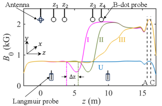
LAPD was used to produce an long cylindrical plasma column (Gekelman et al., 2016). Electromagnets arranged coaxially along the cylindrical vacuum vessel were used to generate a background axial magnetic field, . Plasma was formed through electron impact ionization of Helium by applying a discharge voltage between a mesh anode and a cathode located at the far end of the machine, as shown in Fig. 1.
For our experiments, a two cycle linearly polarized Alfvén wave of azimuthal mode number was excited using an orthogonal ring antenna placed on the cylindrical axis of LAPD at (Gigliotti et al., 2009; Karavaev et al., 2011; Bose et al., 2019). Triaxial B-dot probes at , , , and were used to make wave magnetic-field measurements (Everson et al., 2009; Bose et al., 2018).
We studied reflection of Alfvén waves by varying and . The wave frequency was changed to vary , while different gradients were employed to alter . The four profiles used for the reflection experiments are shown in Fig. 1.
A Langmuir probe was used to measure and for the gradient cases (Hershkowitz et al., 1989; Bose et al., 2017). The density measurements were calibrated using an interferometer that measured line-integrated density. For the gradient cases, the estimated plasma parameters at are and , while at , they are and . We do not have Langmuir probe measurements for the uniform case; the estimated from the Alfvén wave dispersion relation is .
3.2 Detection of an Alfvén wave reflected from a gradient
We performed a number of wave experiments to detect a reflected Alfvén wave from a gradient and validate the findings. We first studied the wave propagation through a uniform as a control case (profile U in Fig. 1). Second, we excited an Alfvén wave in the presence of a strong gradient (profile I in Fig. 1) and detected a reflected wave from the gradient. Third, we pushed the gradient further from the antenna (profile II in Fig. 1) and found the phase difference between the incident and reflected wave increased, confirming that the gradient is the reflector. Fourth, we weakened the gradient significantly (profile III in Fig. 1); we could not find a reflected wave from this gradient, proving that reflection is a gradient-driven effect. In the subsubsections below, we describe the results and analysis of these experiments using an incident wave as an example.
3.2.1 Alfvén wave in uniform
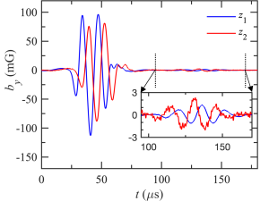
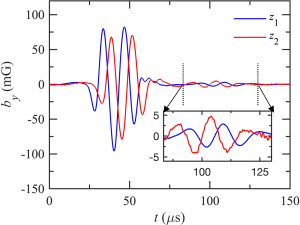
Figure 2 shows the wave magnetic field time series recorded by B-dot probes at and for gradient U. Initially, the peaks and troughs of the wave signal at leads , which is consistent with an incident wave propagating in the direction. Some time after the incident wave in Fig. 2, we see a much smaller wave in the region between the dotted lines. The signal of this smaller wave is observed at before , indicating the waveform is propagating in the direction, towards the antenna.
Our analysis suggests that the smaller wave signal is reflected from the plasma source at the far end of LAPD. Furthermore, reflection introduces an additional phase difference between the reflected and incident wave; the smaller signal in Fig. 2 has three peaks and two troughs, while in the incident wave has two peaks and three troughs. We performed time-of-flight calculations using the logic that if the smaller wave at is reflected from the plasma source, then the time lag between the incident and the inverted smaller wave should be equal to twice the time of flight of the incident wave from to the plasma source. The time lag () between the incident and the smaller waves obtained from their phase difference at is . The error bar represent the uncertainty obtained by calculating the standard deviation of the time lag measured at various radial locations. The time of flight () of the incident wave from to the plasma source determined by dividing the distance between and the cathode, 14.31 m, by the velocity of the wave. The velocity of the wave is , as determined by dividing the distance between and by the time lag between the wave signals at those two locations. Therefore, is . Hence, agrees with , indicating that the smaller wave has been reflected from the plasma source. Our findings agree with previous experiments where physical objects in the plasma, such as metal and insulator plates, were found to reflect Alfvén waves (Leneman, 2007).
3.2.2 Wave reflection from a strong gradient
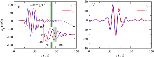
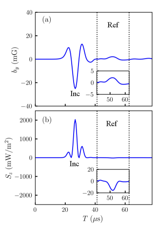
We introduced a strong gradient between the antenna and the far end of LAPD and detected a wave reflected from the gradient. The minimum value of the length scale within the gradient was . The wave magnetic field data before the gradient is given in Fig. 3(a). Initially, the peaks and troughs of the wave signal at leads , which is expected for an incident wave. However, in the region between the dotted lines, a small wave signal is observed at before , suggesting the wave is propagating in the direction. This is likely due to a partial superposition of waves reflected from gradient I and the plasma source, as we explain shortly. Here we remind the reader that since , the time window for the wave reflected by the plasma source at and for the strong gradient and uniform profile will be different as the values of near the plasma source is different in the two cases.
In order to help disentangle wave reflection from the gradient from wave reflection by the plasma source, we also measured the wave magnetic field on the high field side at and (Fig. 3(b)). The first two peaks and troughs at leads , which is consistent with wave propagation in the direction. However, the third trough of lags , suggesting the presence of a wave reflected from the far end in the measured signal. The amplitude of the third trough at is also more than at , suggesting constructive interference between waves travelling in the (incident) and (reflected from far end) directions. The presence of a far-end reflected wave is also supported by the amplitude of the third peak at , which is greater than . This observation suggests that the far-end reflected wave may have reached around . The upper limit corresponds to the time of the second peak at , where we observe a signature of a reflected wave from the far end. The lower limit refers to the time of the second trough at where we do not observe a sign of reflection from the far end.
Building on this, we put forward two sets of analyses that imply that the first cycle of the wave propagating in the direction at is reflected from gradient I only and does not have any contribution due to far-end reflection. First, we estimate the time at which a wave reflected from the plasma source will reach . The arrival time of the reflected wave from the source is equal to plus the time of flight of the wave from to . Since the speed of Alfvén wave propagation in the and direction is the same, the time of flight of an Alfvén wave from to (i.e., the direction) is determined from the phase difference of the incident wave (i.e., the direction) between and . The inferred time of flight is . Therefore, the part of the waveform at beyond may contain a contribution from a wave reflected from the plasma source. Hence, the first cycle of the waveform in the inset graph of Fig 3(a) is not affected by reflection from the source.
Next, we show that the location of reflection of the first cycle of the wave propagating in the direction at is within gradient I. Since gradient I is located between and , for the first cycle to be reflected from the gradient I, the time lag between the incident and reflected wave at , , must be less than the twice the time of flight of the wave from to , . We used the results of the simulations given in Section 4 to correlate the phases of incident and gradient-reflected wave. Simulations showed that reflection from a gradient introduces a phase difference between the incident and the reflected wave. In addition, the simulations also suggest that the leading low amplitude trough of the incident Alfvén wave may not produce a sufficiently strong reflected wave to be experimentally detectable. The subsequent peaks and troughs of the incident Alfvén wave, though, are predicted to produce a detectable reflected wave. Therefore, in Fig. 3(a), the first peak of the incident wave should correspond to the first trough of the wave moving in the direction if it is reflected from the gradient. The time lag between the first peak of the incident wave and the first trough of the reflected wave is . The time of flight of the wave from to obtained by comparing the phase difference between the propagating part of the wave at and is . Hence, indicating that the source of reflection is located within gradient I. This experimental finding is supported by our simulations described in Section 4.
3.2.3 Wave reflection experiment by changing the location of a strong gradient
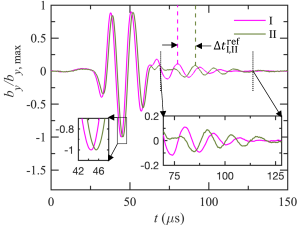
To further confirm experimentally that gradient I is indeed reflecting an Alfvén wave, we moved the gradient further away from the antenna and checked if the time lag between the incident and reflected wave increased accordingly. We refer to this shifted gradient as gradient II. A comparison of the wave signal at for gradients I and II is presented in Fig. 4.
We performed further analysis to quantitatively show that the phase difference between the reflected wave from gradients I and II agrees with the extra distance traversed by the wave to reach gradient II and return. The investigation was done using the first wave cycle propagating in direction for both gradients. This is because an analysis for gradient II following the methodology in subsection 3.2.2 that was used for gradient I showed that the reflector for the first cycle is located within the gradient II region. The time lag between waves reflected from I and II is , where is the distance between gradients I and II (Fig. 1), and is the phase velocity of the Alfvén wave parallel to in the low-field side. We find = , as determined by dividing the distance between and by the phase difference of the incident wave at and . This gives, . The phase difference between the reflected wave from I and II is . In Fig. 4, we find a minor phase offset between the incident waves for cases I and II possibly due to small difference in density. This minor phase offset adds to the phase difference between the reflected waves from the two gradients. Correcting for the phase difference between incident waves, we find . Thus, closely agrees with further confirming that the gradient is reflecting Alfvén waves. This experimental finding is supported by our simulation discussed in Section 4.
3.2.4 Alfvén wave incident on a weak gradient
As a further test to prove that the first cycle of the reflected wave in Fig. 3(a) is a gradient driven effect, we weakened the gradient and repeated the experiment. The within the gradient was . The wave magnetic field data at and for III is shown in Fig. 5. Initially, the troughs and peaks of the wave signal at leads , which is consistent for a wave propagating in the direction. However, some time after the incident wave in Fig. 5, we see a much smaller wave in the region between the dotted lines. This small wave is propagating in the direction, as the peaks and troughs of the small wave at leads .
Analysis shows that the small wave is reflected from the plasma source of LAPD and that there is no signature of the wave being reflected from the gradient. For the small wave to be reflected from the source, the time lag () between the incident and small wave at should be equal to twice the time of flight () of the wave from the to the plasma source. The measured by cross-correlating the incident and small wave after accounting for phase shift caused by reflection is . The time of flight calculated using is . Here, the dependence of primarily causes an axial variation of as , while a minor variation in doesn’t effect much as . Therefore, agrees with to within the measurement uncertainty, proving that the small wave is reflected from the plasma source. Since we do not observe any other wave between the incident wave and the small source-reflected wave in Fig. 5, we conclude that gradient III does not reflect Alfvén waves. This experimental finding is supported by our simulations, which shows that gradient III does not reflect (see Section 4).
3.3 Dependence of reflected Alfvén wave energy on the inhomogeneity
We determined the coefficient of reflection, , to quantify the effectiveness of a gradient in reflecting Alfvén waves. As a first step for determining , we calculate the energy of the incident wave and of the wave reflected from the gradient. The energy, , of an Alfvén wave is obtained by integrating the Poynting vector of the wave and is given by
| (3) |
where is the energy flux along (Bose et al., 2019). The spatial integration is carried out over the cross section of LAPD, and the integration in time, , is carried out over the duration of the wave train.
is obtained from using
| (4) |
where is the wave power, is the time duration of the wave train, and subscripts “” and “” refer to incident and reflected wave, respectively. The quantity consist of the initial ramp-up period and the first full cycle of the incident wave, while is the period of first cycle of the reflected wave. The definition of is motivated by simulation results given in Fig. 8d where a single cycle of the reflected wave is produced by an incident wave comprising of an initial ramp-up followed by a full cycle.
3.3.1 Measurement of coefficient of reflection at
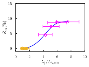
The values of calculated by taking the ratio of the reflected to incident wave power at is given by color filled symbols in Fig. 6, where the magenta and yellow colored data points represent measurements for gradients I and III, respectively. is presented as a percentage by multiplying Eq. 4 by 100. For convenience we have referred to measured at as .
data points for gradient I shows that longer wavelength waves are reflected more strongly from a gradient than shorter wavelengths. The wavelengths were changed by varying the wave frequency. For the longest wavelength, (), and is . For the shortest wavelength, (), and is . Note, the errorbar of is due to uncertainty in frequency measurement which in turn is due to the finite temporal length of the incident wave. We estimated the frequency uncertainty using the full width at half maximum of the frequency peak in the Fourier spectrum of the incident wave.
A comparison of data points for gradients I and III suggests that the length scale of the gradient affects wave reflection. is zero for gradient III, as the measurement of wave magnetic field along the axis spanning the width of the plasma column at did not reveal any signature of a reflected wave from the gradient. However, is non-zero for I. The key difference between I and III are their values of because for both gradients lie in the same range. for I and III are 0.74 m and 3.24 m, respectively. Note that signifies the degree of inhomogeneity of a gradient and a small indicates a strong gradient.
The blue curve in Fig. 6 showing the variation of vs. as predicted by Gaussian process regression (GPR), a class of machine learning algorithms (Rasmussen, 2005). GPR is a Baysean non-parametric regression technique that predicts a probability distribution over possible functions that fit a set of discrete data points. The blue curve in Fig. 6 gives mean of the probability distribution i.e., most probable characterization of the data (Pedregosa et al., 2011; Bose et al., 2022).
3.3.2 Estimating coefficient of reflection in the gradient
The values of in Fig. 6 are the lower limit of the coefficient of reflection. This is because the incident Alfvén wave damps as it propagates from to the location of the reflector in the gradient, causing the incident wave energy to be smaller at the location of the reflector than at . Similarly, the reflected wave damps as it propagates from the site of the reflector in the gradient, causing the reflected wave energy to be smaller at . As a result, the incident wave energy is overestimated while the reflected wave energy is underestimated at compared to the corresponding energies at the site of the reflector in the gradient.
We have used a simple model to estimate the incident and reflected wave energy at the site of the wave reflector to make a zeroth order correction to the directly measured values of . In the model, the incident wave energy at () is related to the incident wave energy at the site of wave reflector () by
| (5) |
where is the distance between and location of the reflector, and is the collisional damping length of Alfvén wave, i.e., the length over which the Alfvén wave amplitude decreases to of its initial value. Note, the factor 2 appears in the exponential term of Eq. (5) because and the damped amplitude of . Similarly, the reflected wave energy at the reflector () and at () are related by
| (6) |
Therefore, the coefficient of reflection at the site of the reflector () is given by
| (7) |
The collisional damping length is estimated using the two-fluid dispersion relation of Alfvén wave for uniform plasma in the limit, (Vranjes et al., 2006; Gigliotti et al., 2009; Bose et al., 2019)
| (8) |
This quadratic equation can be solved algebraically, and the imaginary root, , gives the damping length,
| (9) |
The dominant perpendicular wavelength of the incident wave, . The average value of the plasma parameters between and the reflector are employed for estimating using Eq. 9. The site of reflector is taken to be location of the strongest part of the gradient, which is at , therefore, . The average between and is 623 G. The values of for 61, 76, 89 and 104 kHz waves are 11.4, 11.2, 11, and 10.6 m, respectively.
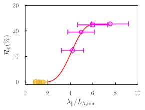
The resulting value of has a monotonic variation with respect to as shown in Fig. 7. The data points are shown by symbols while the red curve is most probable characterization of the data points as per GPR. The vs. curve shows that as the inhomogeneity increases, so does the reflection of Alfvén waves.
The values of are approximate quantities as we estimated of the Alfvén wave in the gradient using the dispersion relation for a uniform plasma. A comprehensive analysis to accurately determine in a strong non-WKB gradient relevant to our experiments is beyond the scope of this paper. However, past experiments of Bose et al. (2019) does provide an insight on the damping of Alfvén waves in a strong non-WKB gradient. They found the energy reduction of an Alfvén wave in a strong non-WKB gradient to be more than in an almost uniform plasma suggesting that the damping length is smaller (i.e. damping is more pronounced) in the gradient than in the uniform case. This implies that for the uniform plasma the values of used to calculate overestimates the damping length in the gradient and thus underestimates . Therefore, in Fig. 7 is likely to be a lower bound on the coefficient of reflection after correcting for collisional damping.
4 Simulations
4.1 Overview
We employ the five-moment, two-fluid model (Hakim et al., 2006; Wang et al., 2015, 2020) within the Gkeyll simulation framework to model Alfvén-wave reflection in LAPD. The five-moment model evolves equations for density, momentum, and isotropic pressure for each species, which are coupled through Maxwell’s equations, and includes the displacement current. We model the full LAPD domain in Cartesian coordinates with reflecting boundary conditions in each dimension, and , and employ and cells. We initialize a Helium plasma, , with g and a reduced mass ratio, , uniform temperatures and densities based on fiducial values from the experiments, eV, , and . The speed of light for simulations is taken to be . Three background, axial magnetic field profiles are employed corresponding to field profiles U, I, and III in Fig. 1. We drive the plasma with a model of the Arbitrary Spatial Waveform (ASW) antenna placed at (Thuecks et al., 2009; Drake et al., 2013). The antenna parameters are , , and , which drives an Alfvén wave with . The antenna is driven for a time . This includes ramping up and down periods, each of length . We note that we both extend the LAPD-model domain to and flatten the background magnetic field gradient in this region to reduce spurious reflections from behind the antenna.
4.2 Results
4.2.1 Alfvén wave through uniform
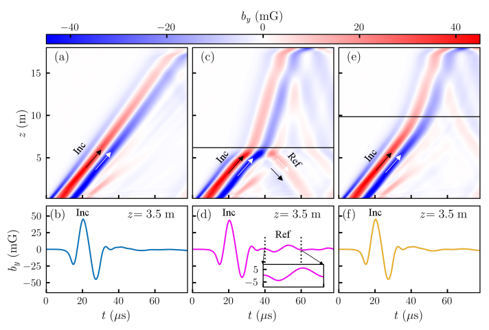
Fig. 8(a) shows the wave propagation along the cylindrical axis of LAPD in the -plane for gradient U. The color gives the -component of the wave magnetic field, which in turn also indicates the phase of the wave. The slope of the band traced by the phase of the wave indicates the propagation direction of the wave; positive and negative slope corresponds to and direction, respectively. In Fig. 8(a), the slope of the band traced by the phase of the wave is positive, consistent for an incident wave propagating away from the antenna. Fig. 8(b) shows the time variation of the incident wave at . Unlike the experiment, we do not see a wave reflected from the far end in the time series data because the simulation was carried out up to , and the wave reflected from the far end requires a longer time to reach .
4.2.2 Alfvén wave reflection from a strong gradient
Fig. 8(c) shows the wave propagation in the -plane for gradient I, where we observe experimentally wave reflection from the gradient. Initially, from to and , the wave propagates in direction as expected for an incident wave. Upon reaching the gradient region, where , a portion of the incident wave is reflected. The negatively sloped arrows trace the phases of the wave reflected from the gradient.
We observe that reflection from a gradient introduces a phase difference between the wave magnetic field of the incident and the reflected wave. In Fig. 8(c), the deep blue band of the incident wave, marked by the positively sloped white arrow, correlates to the negatively sloped red band (reflected wave), marked by the negatively sloped white arrow. Similarly, the positively sloped deep red band of the incident wave corresponds to the negatively sloped blue band of the reflected wave, as shown by . The change in the color between the corresponding phases of the incident and the reflected wave represents a phase difference. We performed a second test to check the phase difference. Simulations using an incident wave having only a strong negative (i.e. no strong positive ) gave rise to a reflected wave with only a positive , further demonstrating a phase difference between incident and reflected wave due to reflection. See Appendix A for the additional details on this second test.
The time variation of before the gradient at in Figs. 8 (c) and (d) show that the first low amplitude trough of the incident wave does not produce a strong detectable reflected wave. The reasons for this observation may be related to the process associated with Alfvén wave reflection at the boundary, such as establishing currents at the boundary to support a reflected Alfvén wave. A discussion on the interaction of the Alfvén wave with the gradient boundary is beyond the scope of this paper and will be discussed elsewhere.
4.2.3 Alfvén wave incident on a weak gradient
Fig. 8(e) shows the wave propagation in the -plane for case III, i.e., the profile with gradient III. We do not observe any wave reflection from the gradient, but the transmitted wave is reflected from the far end of the simulation domain. The time series data in Fig. 8(f) only shows a well-formed incident wave and does not exhibit any signature of a reflected wave from the gradient.
5 Discussion
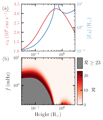
Our experimental results have implication on the heating of coronal holes. A significant temperature increase of coronal hole plasma occurs at low heights (Ko et al., 1997; Landi, 2008), a region where is highly non-uniform. The spatial variation of is shown by the red curve in Fig. 9(a). We used approximate fits of density and magnetic field given by Cranmer & Van Ballegooijen (2005) to calculate .
A comparison of the wave inhomogeneity parameter () for a coronal hole with that of the laboratory suggest that can be greater than at low heights. The spatial variation of and in a coronal hole are given by the red and blue curves, respectively, in Fig. 9(a). The at different heights in a coronal hole for various wave frequencies , can be estimated using . The values of vary from 0.2 to 10 mHz (Morton et al., 2015). The resulting values of were used to obtain estimates of for a coronal hole by comparing of a coronal hole with of the laboratory (red curve in Fig. 7). Fig. 9(b) shows for different values of at various heights above the surface of the Sun. The different shades of red show the values of from 0 to , while the grey indicates . The reason for using the grey color is that in a portion of the frequency-height plane the coronal hole values of are greater than the maximum value of attained in the laboratory. Since, the coefficient of reflection has a monotonic dependence on in the laboratory with a maximum value of we assumed that is in a coronal hole for .
A comparison of the data in Fig. 9b with solar observations and solar simulations suggests that wave reflection from a smooth gradient may be sufficient to significantly heat the plasma at low heights up to in coronal holes via the wave turbulence model. Solar observation suggest that waves have sufficient energy to heat a coronal hole (McIntosh et al., 2011). Furthermore, measurement of the wave frequency spectrum by Morton et al. (2015) indicates that bulk of the wave energy occur at frequencies below in a coronal hole. Simulations of Asgari-Targhi et al. (2021) suggests that a reflection coefficient of may be sufficient to heat the plasma at heights below in coronal holes. They invoked density fluctuations to reflect of the wave power. However, our laboratory results suggest that a smooth gradient relevant to low heights in coronal holes can reflect more than of wave power. In Fig. 9(b) is greater than for for a height up to . Therefore, wave turbulence driven by nonlinear interaction between outward propagating waves from the Sun’s surface and inward reflected waves may heat a coronal hole plasma enough to sustain temperature in lower corona up to a height of .
Although tends to decrease above , reflection may still continue to play a role in heating the plasma at heights up to . The frequency spectrum of Alfvénic waves measured by Morton et al. (2015) suggest the wave energy is concentrated in frequencies at the lower end of the spectrum. In their measurement, the wave energy peaked at , which was the lowest frequency in their dataset. In Fig. 9(b) waves of frequency have up to a height of . The value of for wave frequencies above 0.2 mHz progressively decreases from to . These two features of Fig. 9(b) suggest that wave reflection from the smooth gradient will play a partial role in heating the plasma via a wave turbulence mechanism but that the the role of reflection is expected to progressively decrease with height from to . At heights above , reflection from the smooth gradient is rather weak and the reflected wave may not be of consequence in heating the plasma.
6 Summary
In this paper, we report the first experimental detection of a reflected Alfvén wave from a strong gradient using a series of experiments in solar-like plasmas. Our results show that a strong gradient is necessary to reflect Alfvén waves, and that the reflected wave energy increases for incident waves having longer wavelengths. The trend in the laboratory wave reflection data agree with the solar observation of Morton et al. (2015), where they showed that the ratio of the outward propagating wave power to the inward propagating wave power increases for longer wavelength waves, i.e., smaller wave frequencies. This indicates that the counter-propagating waves observed by Morton et al. (2015) may be due to wave reflection, supporting their hypothesis.
Two-fluid simulations using the Gkeyll code qualitatively agree with and support the experimental detection of a reflected Alfvén wave. In the simulations, we excited Alfvén waves using a model of the ASW antenna. We traced the propagation of Alfvén waves along the plasma column through a uniform profile, as well as strong and weak gradients. Like the experiments, the simulations show that a strong gradient reflects, while a weak gradient does not. In the future, we will make quantitative comparison after developing a model of an orthogonal ring antenna for simulations similar to the one used in experiment.
We experimentally measured for different values of and presented two sets of values of , i.e., and . is determined by dividing the measured reflected wave power just after the wave exits from the gradient region by the incident wave power that enters the gradient region. The gradient region is of finite spatial extent, and since simulations showed that wave reflects from the vicinity of the strongest part of the gradient, we estimated the coefficient of reflection near the strongest part, , using and a model to take into account collisional damping between the edge of the gradient region and the center of the gradient region. The values of and were found to increase with increasing .
A comparison of the laboratory results and solar parameters suggest that Alfvén waves will be reflected by the smooth gradient at heights up to in coronal holes. Furthermore, solar models suggest that the coefficient of reflection may be sufficient to generate enough inward propagating waves at low heights in a coronal hole ( ) to turbulently heat the plasma at these heights. The role of wave reflection from the smooth gradient in heating the plasma is expected to progressively diminish from a height of to . In addition, at heights of or above, reflection from this gradient may not be adequate to generate enough plasma heating via wave turbulence mechanism requiring other processes like density fluctuation to enhance wave reflection (Shoda et al., 2019; Asgari-Targhi et al., 2021).
Appendix A Phase relationship between incident and reflected wave
We performed additional simulations to test the phase relationship between the incident and reflected waves. Profile I was used for the simulations, where the Alfvén wave propagated from a region of low to high velocity. An incident wave having a strong negative was found to produce a reflected wave having a positive , as shown in Fig. 10(a). The direction of propagation of the wave was confirmed by calculating the component of the Poynting vector, , given in Fig. 10(b). A positive value of signifies propagation in the direction, which is consistent for an incident wave. A reflected wave propagating in the direction has a negative value. Therefore, Fig. 10(a) and (b) demonstrates that Alfvén wave reflection from gradient I introduces a phase difference between the incident and reflected wave.
The result of the Alfvén wave reflection simulations agree with the predictions of theory of reflection of light (Griffiths, 2015). According to which, the phase of the magnetic field of a light wave incident on a gradient from the low velocity side is inverted by upon reflection. The reason for the similarity between Alfvén and light waves may be because both are electromagnetic waves.
Acknowledgements
This work was supported by US DOE Frontier Plasma Science program and General plasma science program funded by contract number DE- AC0209CH11466. J.M.T. was additionally supported by the NSF CSSI (Cyberinfrastructure for Sustained Scientific Innovation) program, grant number 2209471. D.W.S. and M.H. were supported by the DOE grant DE-SC0021261. J. Juno was supported by the U.S. Department of Energy under Contract No. DE-AC02-09CH1146 via an LDRD grant. The experiments were performed at the Basic Plasma Science Facility (BaPSF), which is a colaborative research facility supported by the DOE and NSF, with major facility instrumentation developed via an NSF award AGS–9724366. The simulations presented in this article were performed on computational resources managed and supported by Princeton Research Computing, a consortium of groups including the Princeton Institute for Computational Science and Engineering (PICSciE) and the Office of Information Technology’s High Performance Computing Center and Visualization Laboratory at Princeton University.
The United States Government retains a non-exclusive, paid-up, irrevocable, world-wide license to publish or reproduce the published form of this manuscript, or allow others to do so, for United States Government purposes.
Data availability statement
The experimental data presented in this paper will be made available upon publication using Princeton’s data repository. Gkeyll is open source and can be installed by following the instructions on the Gkeyll website (http://gkeyll.readthedocs.io). The input and LAPD gradient files for the Gkeyll simulations presented here are available in the following GitHub repository, https://github.com/ammarhakim/gkyl-paper-inp.
References
- Alfvén (1942) Alfvén, H. 1942, Nature, 150, 405, doi: 10.1038/150405d0
- Asgari-Targhi et al. (2021) Asgari-Targhi, M., Asgari-Targhi, A., Hahn, M., & Savin, D. 2021, The Astrophysical Journal, 911, 63, doi: 10.3847/1538-4357/abe9b4
- Bemporad & Abbo (2012) Bemporad, A., & Abbo, L. 2012, The Astrophysical Journal, 751, 110, doi: 10.1088/0004-637X/751/2/110
- Bose et al. (2019) Bose, S., Carter, T., Hahn, M., et al. 2019, The Astrophysical Journal, 882, 183, doi: 10.3847/1538-4357/ab2fe0
- Bose et al. (2022) Bose, S., Fox, W., Ji, H., et al. 2022, Conversion of magnetic energy to plasma kinetic energy during guide field magnetic reconnection in the laboratory
- Bose et al. (2018) Bose, S., Kaur, M., Barada, K. K., et al. 2018, European Journal of Physics, 40, 015803, doi: 10.1088/1361-6404/aaee31
- Bose et al. (2017) Bose, S., Kaur, M., Chattopadhyay, P., et al. 2017, Journal of Plasma Physics, 83, 615830201, doi: 10.1017/S0022377817000289
- Braginskii (1965) Braginskii, S. I. 1965, Review of Plasma Physics, 1, 205
- Breun et al. (1987) Breun, R., Brooker, P., & Brouchous, D. 1987, in Plasma physics and controlled nuclear fusion research 1986 (International Atomic Energy Agency). https://inis.iaea.org/search/search.aspx?orig_q=RN:18091939
- Chandran & Hollweg (2009) Chandran, B. D., & Hollweg, J. V. 2009, The Astrophysical Journal, 707, 1659, doi: 10.1088/0004-637X/707/2/1659
- Churchill & Brown (1987) Churchill, R., & Brown, J. 1987, Fourier Series and Boundary Value Problems, 4th edn. (McGraw-Hill)
- Cramer (2011) Cramer, N. 2011, The Physics of Alfvén Waves (Wiley-VCF)
- Cranmer (2009) Cranmer, S. R. 2009, Living Reviews in Solar Physics, 6, 3, doi: 10.12942/lrsp-2009-3
- Cranmer et al. (2015) Cranmer, S. R., Asgari-Targhi, M., Miralles, M. P., et al. 2015, Philosophical Transactions of the Royal Society of London Series A, 373, 20140148, doi: 10.1098/rsta.2014.0148
- Cranmer & Van Ballegooijen (2005) Cranmer, S. R., & Van Ballegooijen, A. 2005, The Astrophysical Journal Supplement Series, 156, 265, doi: 10.1086/426507
- Cranmer et al. (2007) Cranmer, S. R., Van Ballegooijen, A. A., & Edgar, R. J. 2007, The Astrophysical Journal Supplement Series, 171, 520, doi: 10.1086/518001
- Cross (1988) Cross, R. 1988, An Introduction to Alfvén Waves,, Adam Hilger series on plasma physics (Taylor & Francis)
- Del Zanna et al. (2001) Del Zanna, L., Velli, M., & Londrillo, P. 2001, Astronomy & Astrophysics, 367, 705
- Dmitruk et al. (2001) Dmitruk, P., Milano, L. J., & Matthaeus, W. H. 2001, The Astrophysical Journal, 548, 482, doi: 10.1086/318685
- Drake et al. (2013) Drake, D. J., Schroeder, J. W. R., Howes, G. G., et al. 2013, Phys. Plasmas, 20, 072901, doi: 10.1063/1.4813242
- Everson et al. (2009) Everson, E., Pribyl, P., Constantin, C., et al. 2009, Review of Scientific Instruments, 80, doi: 10.1063/1.3246785
- Fludra et al. (1999) Fludra, A., Del Zanna, G., Alexander, D., & Bromage, B. 1999, Journal of Geophysical Research: Space Physics, 104, 9709, doi: 10.1029/1998JA900033
- Gekelman et al. (1997) Gekelman, W., Vincena, S., Leneman, D., & Maggs, J. 1997, Journal of Geophysical Research: Space Physics, 102, 7225, doi: 10.1029/96JA03683
- Gekelman et al. (2011) Gekelman, W., Vincena, S., Van Compernolle, B., et al. 2011, Physics of Plasmas, 18, 055501, doi: 10.1063/1.3592210
- Gekelman et al. (2016) Gekelman, W., Pribyl, P., Lucky, Z., et al. 2016, Review of Scientific Instruments, 87, 025105, doi: 10.1063/1.4941079
- Gigliotti et al. (2009) Gigliotti, A., Gekelman, W., Pribyl, P., et al. 2009, Physics of Plasmas, 16, 092106, doi: 10.1063/1.3224030
- Goossens et al. (2012) Goossens, M., Andries, J., Soler, R., et al. 2012, The Astrophysical Journal, 753, 111, doi: 10.1088/0004-637X/753/2/111
- Goossens et al. (2009) Goossens, M., Terradas, J., Andries, J., Arregui, I., & Ballester, J. 2009, Astronomy & Astrophysics, 503, 213, doi: 10.1051/0004-6361/200912399
- Griffiths (2015) Griffiths, D. 2015, Introduction to Electrodynamics (Pearson India Education Services Pvt, Ltd.)
- Hahn et al. (2018) Hahn, M., D’Huys, E., & Savin, D. W. 2018, The Astrophysical Journal, 860, 34, doi: 10.3847/1538-4357/aac0f3
- Hahn et al. (2022) Hahn, M., Fu, X., & Savin, D. W. 2022, The Astrophysical Journal, 933, 52, doi: 10.3847/1538-4357/ac7147
- Hahn et al. (2012) Hahn, M., Landi, E., & Savin, D. W. 2012, The Astrophysical Journal, 753, 36, doi: 10.1088/0004-637X/753/1/36
- Hahn & Savin (2013) Hahn, M., & Savin, D. W. 2013, The Astrophysical Journal, 776, 78, doi: 10.1088/0004-637X/776/2/78
- Hakim et al. (2006) Hakim, A., Loverich, J., & Shumlak, U. 2006, J. Comp. Phys., 219, 418, doi: 10.1016/j.jcp.2006.03.036
- Hara (2019) Hara, H. 2019, The Astrophysical Journal, 887, 122, doi: 10.3847/1538-4357/ab50bf
- Hershkowitz et al. (1989) Hershkowitz, N., Auciello, O., & Flamm, D. 1989, Plasma diagnostics, 1, 113
- Huba et al. (2016) Huba, J., of Naval Research, U. S. O., & (U.S.), N. R. L. 2016, NRL Plasma Formulary, NRL publication (Naval Research Laboratory). https://suli.pppl.gov/2016/course/NRL_FORMULARY_16.pdf
- Karavaev et al. (2011) Karavaev, A., Gumerov, N., Papadopoulos, K., et al. 2011, Physics of Plasmas, 18, 032113, doi: 10.1063/1.3562118
- Ko et al. (1997) Ko, Y.-K., Fisk, L. A., Geiss, J., Gloeckler, G., & Guhathakurta, M. 1997, Solar Physics, 171, 345, doi: 10.1023/A:1004943213433
- Landi (2008) Landi, E. 2008, The Astrophysical Journal, 685, 1270, doi: 10.1086/591225
- Leneman (2007) Leneman, D. 2007, Physics of Plasmas, 14, 122109, doi: 10.1063/1.2813459
- Matthaeus et al. (1999) Matthaeus, W. H., Zank, G. P., Oughton, S., Mullan, D. J., & Dmitruk, P. 1999, The Astrophysical Journal Letters, 523, L93, doi: 10.1086/312259
- McIntosh et al. (2011) McIntosh, S. W., De Pontieu, B., Carlsson, M., et al. 2011, Nature, 475, 477, doi: 10.1038/nature10235
- Mitchell et al. (2002) Mitchell, C., Maggs, J., Vincena, S., & Gekelman, W. 2002, Journal of Geophysical Research: Space Physics, 107, doi: 10.1029/2002JA009277
- Moore et al. (1991a) Moore, R., Suess, S., Musielak, Z., & An, C.-H. 1991a, The Astrophysical Journal, 378, 347, doi: 10.1086/170435
- Moore et al. (1992) Moore, R. L., Hammer, R., Musielak, Z. E., Suess, S. T., & An, C. H. 1992, ApJ, 397, L55, doi: 10.1086/186543
- Moore et al. (1991b) Moore, R. L., Musielak, Z. E., Suess, S. T., & An, C. H. 1991b, in Mechanisms of Chromospheric and Coronal Heating, ed. P. Ulmschneider, E. R. Priest, & R. Rosner (Berlin, Heidelberg: Springer Berlin Heidelberg), 435–437, doi: 10.1007/978-3-642-87455-0_73
- Morton et al. (2015) Morton, R., Tomczyk, S., & Pinto, R. 2015, Nature communications, 6, doi: 10.1038/ncomms8813
- Musielak et al. (1992) Musielak, Z., Fontenla, J., & Moore, R. 1992, Physics of Fluids B: Plasma Physics, 4, 13, doi: 10.1063/1.860452
- Narain & Ulmschneider (1996) Narain, U., & Ulmschneider, P. 1996, Space Science Reviews, 75, 453, doi: 10.1007/BF00833341
- Oughton et al. (2001) Oughton, S., Matthaeus, W. H., Dmitruk, P., et al. 2001, The Astrophysical Journal, 551, 565, doi: 10.1086/320069
- Pedregosa et al. (2011) Pedregosa, F., Varoquaux, G., Gramfort, A., et al. 2011, Journal of Machine Learning Research, 12, 2825. http://jmlr.org/papers/v12/pedregosa11a.html
- Priest (2014) Priest, E. 2014, Magnetohydrodynamics of the Sun (Cambridge University Press), doi: 10.1017/CBO9781139020732
- Rasmussen (2005) Rasmussen, C. E. 2005, Gaussian processes for machine learning /, Adaptive Computation and Machine Learning series (Cambridge, Mass. :: MIT Press,), doi: 10.7551/mitpress/3206.001.0001
- Roberts et al. (1989) Roberts, D., Hershkowitz, N., Majeski, R., & Edgell, D. 1989, in AIP Conference Proceedings, Vol. 190, AIP, 462–465, doi: 10.1063/1.38448
- Shoda et al. (2019) Shoda, M., Suzuki, T. K., Asgari-Targhi, M., & Yokoyama, T. 2019, The Astrophysical Journal Letters, 880, L2, doi: 10.3847/2041-8213/ab2b45
- Stix & Palladino (1958) Stix, T. H., & Palladino, R. 1958, The Physics of Fluids, 1, 446, doi: 10.1063/1.1724362
- Swanson et al. (1972) Swanson, D., Clark, R., Korn, P., Robertson, S., & Wharton, C. 1972, Physical Review Letters, 28, 1015, doi: 10.1103/PhysRevLett.28.1015
- Thuecks et al. (2009) Thuecks, D., Kletzing, C., Skiff, F., Bounds, S., & Vincena, S. 2009, Physics of Plasmas, 16, 052110, doi: 10.1063/1.3140037
- Van Doorsselaere et al. (2008) Van Doorsselaere, T., Nakariakov, V., & Verwichte, E. 2008, The Astrophysical Journal Letters, 676, L73, doi: 10.1086/587029
- Vincena et al. (2001) Vincena, S., Gekelman, W., & Maggs, J. 2001, Physics of Plasmas, 8, 3884, doi: 10.1063/1.1389092
- Vincena (1999) Vincena, S. T. 1999, PhD thesis. https://www.proquest.com/openview/eb25033d38437321d239c07204214858/1?pq-origsite=gscholar&cbl=18750&diss=y
- Vranjes et al. (2006) Vranjes, J., Petrovic, D., Poedts, S., Kono, M., & Čadež, V. 2006, Planetary and Space Science, 54, 641, doi: 10.1016/j.pss.2005.12.015
- Wang et al. (2015) Wang, L., Hakim, A. H., Bhattacharjee, A., & Germaschewski, K. 2015, Phys. Plasmas, 22, 012108, doi: 10.1063/1.4906063
- Wang et al. (2020) Wang, L., Hakim, A. H., Ng, J., Dong, C., & Germaschewski, K. 2020, J. Comp. Phys., 415, 109510, doi: 10.1016/j.jcp.2020.109510
- Yasaka et al. (1988) Yasaka, Y., Majeski, R., Browning, J., Hershkowitz, N., & Roberts, D. 1988, Nuclear Fusion, 28, 1765, doi: 10.1088/0029-5515/28/10/005
- Zhang et al. (2008) Zhang, Y., Heidbrink, W., Boehmer, H., et al. 2008, Physics of Plasmas, 15, 012103, doi: 10.1063/1.2827518