Explaining Hierarchical Features in Dynamic Point Cloud Processing
Abstract
This paper aims at bringing some light and understanding to the field of deep learning for dynamic point cloud processing. Specifically, we focus on the hierarchical features learning aspect, with the ultimate goal of understanding which features are learned at the different stages of the process and what their meaning is. Last, we bring clarity on how hierarchical components of the network affect the learned features and their importance for a successful learning model. This study is conducted for point cloud prediction tasks, useful for predicting coding applications.
Index Terms:
dynamic point clouds, hierarchical learning, explanability, predictionI Introduction
One major open challenge in multimedia processing is learning spatio-temporal features for dynamic point cloud (PC) sequences. Being able to extract such information can be essential for future compression algorithms. By learning spatio-temporal features, a predictive motion-compensated coding approach can reduce inter-frames redundancies from the compressed bitstream [1]. Similarly, a PC predictor can be used as learning-based decoder [2]. More at large, spatio-temporal features are important also in high-level PC downstream tasks such as action recognition, prediction and obstacle avoidance. As of today, one of the most successful methodology is to learn features via deep neural networks applied to each point (or group of points) instead of the whole PC. This enables the consumption of the raw PC data directly, without pre-processing steps (e.g., voxelization) that could obscure natural invariances of the data or introduce quantization errors. An example is the pioneer PointNet [3] architecture, which learns global PC features by aggregating local spatial features learned by processing each point independently.
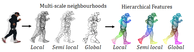
However, in such architecture, the local structures of the PC are neglected. From convolutional neural networks (CNNs), we know that leveraging the local structure is a key aspect of the success of CNNs, in which local features are extracted from small neighborhoods, grouped into larger units, and processed to produce higher level features. This is the well-known “hierarchical feature extraction”, deeply used in 2D computer vision and processing tasks. In PCs, neighboring points form a meaningful subset that captures key semantic information about the 3D geometry; hence they should retain even more information than the 2D counterpart. Because of this intuition, PointNet++ [4] introduced a hierarchical architecture for PC processing, capturing features at increasingly larger scales along a multi-resolution hierarchy. This concept is illustrated in Figure 1, where a PC input is processed at different scales (middle part of the figure) to extract hierarchical features (right side of the figure) at different levels. At the lower level (“Local” in the figure), each point neighborhood covers a small and densely populated region, extracting fine geometric structures. In contrast, at the higher levels (“Global” in the figure), the network captures coarser structures from larger neighborhoods.

Given the increasing importance of dynamic PC sequences in a wide spectrum of applications from automation to virtual reality, several works have extended the PointNet++ network by introducing spatio-temporal neighborhoods in order to learn temporal features. Most of these works adopt hierarchical architectures [5, 6, 7, 8, 9], which can be considered the de-facto approach for dynamic point cloud processing today.
The common intuition is that such hierarchical architecture allows learning more descriptive features, pushing researchers to develop even more hierarchical (and possibly complex) models. However, why such models work and which features do they learn in the framework of PC processing is still not understood and usually overlooked in the literature. Initial understanding has been provided for the PointNet model [3, 10]. However, such efforts are limited to the original PointNet, which does not have a hierarchical learning architecture and it processes static PCs only, leaving a gap in the understanding of current PC processing models. For example, which motion or flow is learned at the different stages of the hierarchical architecture is unknown. Also which key components of the networks (multi-scaling, stacking of deep nets, etc.) lead to the success of the model remain overlooked. Bringing more clarity to such hierarchical learning models when applied to dynamic PC sequences is the goal of this work, which provides a clear understanding of the hierarchical spatial-temporal features extraction in dynamic PCs.
Specifically, we perform an experimental study using state-of-the-art prediction architecture via hierarchical Recurrent Neural Networks (RNN) proposed in Point-RNN [9] and improved in Graph-RNN [7]. To this end, we design different variations of the hierarchical architecture and perform an ablation study across architectures using a dataset of human body motion [11], with the clear intent of disentangling the multi-scale effect from the deep learning one. Then, we explain the learned features for each tested architecture by visualizing the body motion vector. This strategy allows us to demonstrate how learning features at multiple scales is equivalent to extracting local and global temporal correlations from data. This confirms what has been studied in CNN architectures [12]. However, unlike CNNs, in which only the last layer features are processed to infer the final task, we show that all the learned features are important to properly capture complex movements (and perform downstream tasks). In fact, we show that either when the hierarchical learning is not considered or when is considered but only the last level is taken into account, we cannot translate anymore the local and global features to local and global movements and the final task is not properly inferred. While some of these insights might be intuitive, to the best of our knowledge this is the first work validating those intuitions in the dynamic PC setting. Moreover, we believe that understanding the effect of the different components of the network on the features and the prediction accuracy can inform future research directions in how to learn more representative hierarchical features as well as how to take advantage of their combination towards the development of simpler and more accurate methods.
II Background - Hierarchical Architecture
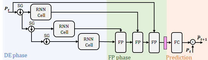
Without loss of generality, we focus on the architecture depicted in Figure 2 for the task of PC prediction [9, 7]. The architecture, which extracts the spatio-temporal features via RNN cells, is composed by two phases:
-
1.
Dynamic Extraction phase (DE): the network processes the input PC frame and extracts its hierarchical features ;
-
2.
Feature Propagation phase (FP): combines the learned features to reconstruct the predicted point cloud , which is the PC at the next time step.
We now describe both phases in more details.
II-1 Dynamic Extraction phase (DE)
The DE phase takes a PC (pre-processed or raw) as input and extracts the PC dynamic behavior. The DE phase consists of multiple stacked RNN cells, for a total of levels. Before being processed by the RNN cell, the PC is downsampled by a Sampling and Grouping (SG) module, as described in [4]. Hence, a progressive subsampled PC is fed into subsequent RNN cells. In each RNN, each point of the cloud is processed jointly with its spatio-temporal neighborhood, defined as its -closest neighbors in space and time. It is worth noting that due to the subsequent sampling (hence a sparser PC at later levels/RNN cells) leads to a neighborhood with larger distances between points. As a result, the first level learns local features from small scale neighborhoods whereas the last level learns global features observing large scale neighborhoods. On top of such multi-scale effect, the stacked RNNs make the model deeper imposing that features learned at each level are the input to the next level . In natural language processing (NLP) the advantage of staking RNN with respect to the vanilla RNN model has been empirically proved [13]. In this work, we aim at understanding if the gain from the stacked effect also remains in PC processing.
II-2 Feature Propagation phase (FP)
Once DE phase has learned the features from all the levels (), the FP phase combines them into a single final feature (). The combination is done by hierarchically propagating the features from the higher levels to the lower levels through several Feature Propagation (FP) [4] modules. This is done by first interpolating the sub-sampled features from the higher level to the same number of points as the lower level, followed by a concatenation of the interpolated features with lower-level features. The concatenation is then processed by a point-based network and a ReLU. The process is repeated in a hierarchical manner until the features from all the levels have been combined into a final feature. As last step, after the FP phase, the final features are converted into motion vectors using a fully connected layer. The calculated motion vectors are then added to the original PC to predict the PC at the next time step.
III Experimental Study
In this section, we present the different architectures along with the dataset and simulation settings used in our study.
III-A Dataset
Similarly to [7], we use the human Mixamo [11] dataset, consisting of sequences of human bodies while performing various dynamic activities such as dancing or playing sports. The main motivations behind this selection are given in the following: compared to real 3D scenes acquired by LiDAR or mmWave sensors, such synthetic dataset does not suffer from acquisition noise or quantization distortion. This makes the dataset easy to visualize and hence to comprehend, while also isolating the problem of learning features from noisy corrections and other aspects that may arise in a more noisy dataset. Additionally, the synthetic dataset allow us to generate very different movements (from quite simply like walking to highly complicating such as breakdance steps) and study the learning of the highly descriptive features in such cases.
III-B Experimental Architectures
To better understand and explain the hierarchical features learning, different architectures have been implemented, trained and compared to the Classic hierarchical architecture depicted in Figure 2. The key idea is to isolate the multi-scale resolution, from the “deepness” of the architecture, disentangling in such a way the different aspects of the PC processing. The common aspects of all implemented solutions is the high level architecture depicted in Section II: a DE phase (with and downsampling factor in SG of four), a FP phase and a final prediction step. On the other side, the models differentiate in the RNN processing (stacked or parallel), as well as in the sampling modules. Specifically, we implemented the following architectures:
-
•
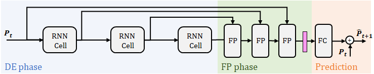
Shallow hierarchical architecture – Figure 3 a): as in Classic architecture, the PC is sub-sampled in a stacked fashion, leading to a very sparse PC at level . Unlike the Classic architecture, the RNN cells are in parallel (instead of stacked), leading to a Shallow network (local features are not grouped and processed at higher levels). This network highlights the effect of multi-scaling (sampling) instead of deep hierarchical learning.
-
•
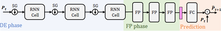
Single-scale architecture – Figure 3 b): Same architecture as in Classic hierarchical model but without the downsampling modules at each level. Hence, all the levels process the same number points and learn features at the same scale.
-
•
Without-combination architecture – Figure 3 c): this architecture recall the classic deep neural network in which local features are extracted from small neighborhoods (first RNN cell) and processed at higher (subsequent) level. Only the last level feature is then used for the final reconstruction. Note that in the Classic architecture all features learned at different level are used for predicting the final motion vectors.
III-C Results Evaluation and Visualization
The above models, as well as the Classic one, are trained using as loss function a combination of the Chamfer distance (CD) [14] and earth’s moving distance (EMD) [14] to measure the distance between predicted and the target PC , as explained in [7]. Those metrics are also used for the evaluation of PC prediction in the experimental results discussion. It is worth noting that the CD distance tends to flatten all scores toward zero values. This is because in the PC the majority of the points are perfectly predicted (all points with no motion or little motion) and most of the errors (high CD scores) are focused in the high motion area. This is the area of strongest interest in PC prediction tasks as we are interested in understanding if the neural network is able to capture such movements. Therefore, we also consider the CD Top 5% metric, which looks at the CD metric of the 5% points with the worst prediction (i.e., points with the farthest distance to their closest point).
Besides the aforementioned metrics, we also visualize the features learned at each level as motion vectors. This is a key aspect to better understand the hierarchical learning process, the goal of this paper. As shown in Figure 2, the motion vectors are obtained by combining features from multiple levels in the FP phase. The final features are then processed by a last fully connected layer and converted into motion vectors. We are interested in visualizing the actual contribution to the final motion vectors from each level. We do this by seeing the motion vectors as the combination of motion vectors produced at each level i.e., , with being the predicted motion vectors and the motion vectors produced by level . Such level contribution is visualized by keeping the features from level and setting to zero the remaining ones at the input of the FP phase. We then replicate the FP and prediction phase operation with the already trained weights and obtain the motion vector generated by level .
IV Explaining hierarchical features
We now present and discuss the results obtained from our study of hierarchical features, which is the core contribution of this work. We aim at explaining what features are learned and how these are learned in the Classic hierarchical architecture. Then, we investigate the role that the combination of hierarchical features has in the dynamic PC processing (by comparing the Classic with those presented above).
IV-A Hierarchical Learning
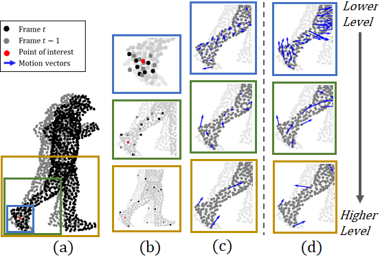
To study hierarchical learning in dynamic PC processing, we study the features learned from the Classic architecture in Figure 2. We visualize those features giving as input PC a running person shown in Figure 4. We investigate how each level of the architecture learns features for a given point of interest, such as a point in the foot (red point in the Figure 4). To do so, we first show in Figure 4 b) the multi-scale neighborhood of the selected point in the foot at each level. Due to the subsequent sampling in the network, the lower level learns features only by looking at points in a small area around the point of interest (top blue square in the figure). On the contrary, the higher level learns features by considering a sparser set of points in a large area (bottom gold square in the figure). In Figure 4 c), we visualize the motion vectors at each level of the Classic hierarchical architecture for given time frame . It can be observed that the lowest level captures small and diverse motions; on the contrary, at the highest level, a single main motion vector is learned for almost all the points in the foot. Similarly to what happens in hierarchical CNNs, we observe that the highest level of the network learns global motions (for example the forward motion of the runner), while lower levels of the architecture learn local movements of the action (small refinement motion that defines the local movement of the foot – which can also go up-backward when the foot goes up). While intuitive, to the best of our knowledge, this visualization is the first one in the literature confirming that the intuition behind hierarchical features in CNNs can be extended to dynamic PCs architectures and dynamic flow: hierarchical features can be explained as local and global motions.
To carry out our deeper understanding of hierarchical learning, now we want to answer the following questions: How does the hierarchical architecture learn global and local motion? (Sections IV-B and IV-C); How does the hierarchical PC architecture differ from CNN? (Section IV-D).
IV-B Is Stacked Effect the key?
To understand better how global and local motions are learned in the hierarchical architecture, we first investigate the effect of the stacked component on the learned features. To do so, we compare the Classic architecture (in which local features are aggregated and processed at a higher level) to the Shallow one, which learns features without features aggregation. Note that in both architectures there is the multi-scaling effect, with the higher lever observing a much sparser PC (hence processing a more global neighborhood). Looking at the motion vectors learned in the Shallow (Figure 4 d)) architecture, we can note that 1) motion vectors are all at the same magnitude across levels; 2) at higher levels the vectors show highly contrasting movements. This implies that in the Shallow architecture the features lose the global and location motion interpretation. Specifically, we do not have the global motion (runner moving forward) being captured by the higher levels. Similarly, lower levels do not capture only small and refining local motions. This is motivated by the fact that in the Shallow architecture all three levels contribute equally to the output motion. This proves that the features interpretation is not guaranteed by the multi-scale component in the architecture, while it is learned by the stacked aspects of local features being aggregated and processed to learn global motion.
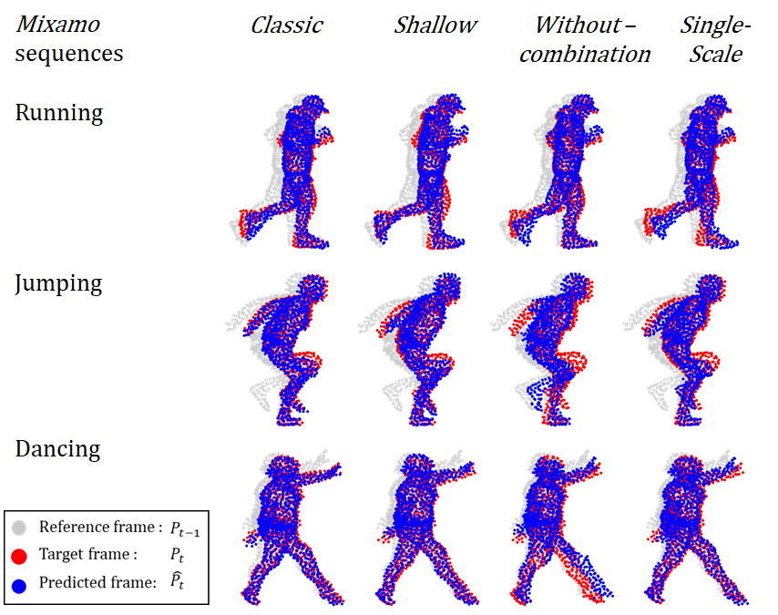
Interestingly, we have also observed that despite the missing interpretation of global and local motion, the Shallow can capture the overall movement of the PC and perform a decent prediction. This is observed in Table I, which shows the prediction error for the different architectures presented in Section III-B. We also add the prediction error for the “Copy-Last-Input” case, in which the prediction is simply the copy of the previous input. This shows that all the methods investigated in this work perform substantially better than “Copy-Last-Input”, hence they are all able to capture some aspects of the body movements. We also visualise in Figure 5 the prediction for three particular sequences: Running, Jumping, and Dancing. We can observe that the Dancing PC is very well predicted from both Shallow and Classic architectures. In Jumping and Running sequences, there is a mild gain from the Classic one (see for example the arm in Jumping) but the Shallow architecture still learns well the overall movement. In short, while the stacked aspect has a big impact on the interpretation of the learned feature, the performance gap is not as substantial.
IV-C Is Multi-Scale Effect the key?
We are now interested in understanding how much the multi-scale effect is important for capturing the PC motion. We compare the Classic architecture to the Single-scale architecture (i.e., without multi-scale effect) and we show that the multi-scale is essential to achieve a good performance (hence prediction). This is confirmed both numerically and visually. In Table I, the Classic architecture has a better overall prediction accuracy and from Figure 5, it is clear that Single-scale architecture fails in capturing some local movements such as the foot/leg in “Running”, the knee in “Jumping” and the hands in “Dancing”. This is motivated by the following: in complex movement, as in the “Running”, in which the foot performs a forward translation and rotation motion simultaneously (Figure 4 c), the joint-motion can be captured only by looking at points from different scales, the forward movement required a large-scale neighborhood for example. Only by observing the foot neighborhoods at multiple scales both the global forward motion and local rotation motion are captured. This ability to capture complex motion patterns as local and global motions results in more accurate predictions.
IV-D Is This Like Any Other Deep Learning?
We are now interested in answering the second question: How does the hierarchical PC architecture differ from CNN? Both architectures use a hierarchical approach to learn global and local features. However, in CNNs only the last layer features are usually processed to infer the final task, while in the Classic architecture all features from all the levels are combined in an FP propagation phase. We then compare the Classic architecture to the Without-combination one, which does not combine the features from different levels. From Figure 5, we can already observe that the Without-combination architecture fails in predicting key local movements: knee in “Jumping” and leg in “Dancing”. Even if the network can learn hierarchical features, it is not able to merge the local motions in the final reconstruction, in which only the higher level motion is used for the prediction. As a result, the network loses the ability to predict complex motions, resulting in an inferior performance (validated in Table I).
| Experimental Architectures | CD | EMD | CD Top 5% |
|---|---|---|---|
| Classic | 0.00262 | 59.6 | 0.1412 |
| Shallow | 0.00268 | 62.2 | 0.1459 |
| Single-scale | 0.00331 | 65.0 | 0.1609 |
| Without-combination | 0.00314 | 67.3 | 0.1752 |
| Copy-Last-Input | 0.01056 | 123.4 | 0.2691 |
V Conclusion
By performing an experimental study on state-of-art architectures for PC prediction, this paper explains hierarchical features in the context of dynamic PC processing. Specifically, we have shown 1) the interpretation of low- and high-level features as local and global motions; 2) the importance of different components of the networks in current state-of-the-art models to achieve a better PC predictions. We believe that such insights can open the door to new designs of more efficient and accurate networks for future PC processing tasks such as learning-based PC compression algorithms.
References
- [1] D. Thanou, P. A. Chou, and P. Frossard, “Graph-based compression of dynamic 3d point cloud sequences,” IEEE Trans on Image Processing, 2016.
- [2] A. Akhtar, Z. Li, and G. Van der Auwera, “Inter-frame compression for dynamic point cloud geometry coding,” arXiv:2207.12554, 2022.
- [3] C. R. Qi, H. Su, K. Mo, and L. J. Guibas, “Pointnet: Deep learning on point sets for 3d classification and segmentation,” in Proc. IEEE/CVF Conf. on Computer Vision and Pattern Recogn., 2017, pp. 652–660.
- [4] C. R. Qi, L. Yi, H. Su, and L. J. Guibas, “Pointnet++: Deep hierarchical feature learning on point sets in a metric space,” in Proc. Conf. and Workshop on Neural Information Processing Systems, 2017.
- [5] H. Fan, Y. Yang, and M. Kankanhalli, “Point spatio-temporal transformer networks for point cloud video modeling,” IEEE Trans. on Pattern Analysis and Machine Intelligence, 2022.
- [6] H. Fan, X. Yu, Y. Ding, Y. Yang, and M. Kankanhalli, “Pstnet: Point spatio-temporal convolution on point cloud sequences,” in Proc. Int. Conf. on Learning Representations., 2021.
- [7] P. Gomes, S. Rossi, and L. Toni, “Spatio-temporal graph-rnn for point cloud prediction,” in Proc. IEEE Int. Conf. on Image Processing. IEEE, 2021, pp. 3428–3432.
- [8] X. Liu, C. R. Qi, and L. J. Guibas, “Flownet3d: Learning scene flow in 3d point clouds,” in Proc. IEEE/CVF Conf. on Computer Vision and Pattern Recogn, 2019, pp. 529–537.
- [9] H. Fan and Y. Yang, “Pointrnn: Point recurrent neural network for moving point cloud processing,” in arXiv:1910.08287, 2019.
- [10] B. Zhang, S. Huang, W. Shen, and Z. Wei, “Explaining the pointnet: What has been learned inside the pointnet?” in Proc. IEEE/CVF Conf. on Computer Vision and Pattern Recogn, 2019, pp. 71–74.
- [11] Adobe. Mixamo: Animated 3d characters for games, film, and more. [Online]. Available: https://www.mixamo.com/
- [12] M. D. Zeiler and R. Fergus, “Visualizing and understanding convolutional networks,” in Proc. IEEE European Conf. on Computer Vision., 2014, pp. 818–833.
- [13] R. Pascanu, C. Gulcehre, K. Cho, and Y. Bengio, “How to construct deep recurrent neural networks,” in Proc. Int. Conf. on Learning Representations, 2014.
- [14] H. Fan, H. Su, and L. J. Guibas, “A point set generation network for 3d object reconstruction from a single image,” in Proc. IEEE/CVF Conf. on Computer Vision and Pattern Recogn, 2017.