Explaining Object Detectors via Collective Contribution of Pixels

Toshinori Yamauchi¹ Hiroshi Kera² Kazuhiko Kawamoto³ Graduate School of Informatics, Chiba University
¹t.yamauchi@chiba-u.jp, ²kera@chiba-u.jp, ³kawa@faculty.chiba-u.jp

Abstract

Visual explanations for object detectors are crucial for enhancing their reliability. Since object detectors identify and localize instances by assessing multiple features collectively, generating explanations that capture these collective contributions is critical. However, existing methods focus solely on individual pixel contributions, ignoring the collective contribution of multiple pixels. To address this, we proposed a method for object detectors that considers the collective contribution of multiple pixels. Our approach leverages game-theoretic concepts, specifically Shapley values and interactions, to provide explanations. These explanations cover both bounding box generation and class determination, considering both individual and collective pixel contributions. Extensive quantitative and qualitative experiments demonstrate that the proposed method more accurately identifies important regions in detection results compared to current state-of-the-art methods. The code will be publicly available soon.

1 Introduction

Object detectors [38, 7] are applied in various safety-critical domains, such as autonomous driving [22, 60] and medical imaging [30, 2]. To ensure their reliability, it is critical to understand which regions of an image have a significant impact on the detection. If these influential regions are not reasonable to humans, the detector may not be reliable. Various methods have been developed to visualize highly contributing image regions. For example, D-RISE [33] identifies important regions by analyzing input sensitivity to random masks, while spatially sensitive grad-CAM [55] highlights these regions by incorporating spatial information into Grad-CAM [40] outputs.

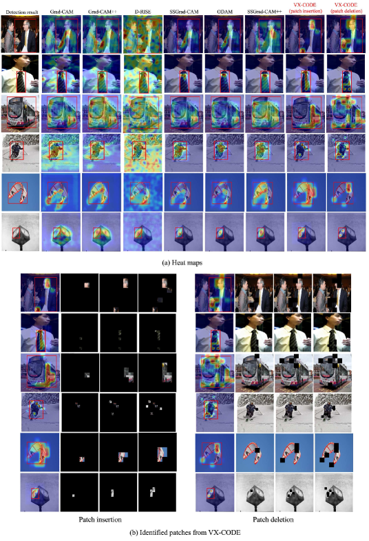
However, existing methods do not consider the collective contributions of image regions to detect, potentially overlooking a compositional detection process or spurious correlations. Figure 1 reveals that state-of-the-art methods cannot capture such collective contributions. For example, as presented in the top row, the detection of a human should be influenced by multiple features, such as the head and legs, which collectively determine the bounding box size and associated class. In contrast, existing methods (ODAM [61] and SSGrad-CAM++ [54]) only highlight the hand. Similarly, as depicted in the bottom row of Fig. 1, in the image of a man surfing in the sea, the detection of the surfboard should be influenced not only by the surfboard itself but also by the man on it and the surrounding sea (sensitivity to features outside the bounding box in object detectors has been explored in several studies [33, 55, 11]). Nevertheless, ODAM and SSGrad-CAM++ highlight only the surfboard, ignoring the collective influence of the surrounding regions. Therefore, accurate visualization that considers the collective contributions of important pixels is essential to explain object detectors.

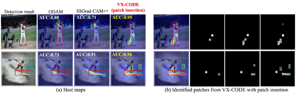
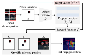
Refer to caption — Figure 1: (a) Generated heat maps are shown for ODAM, SSGrad-CAM++, and VX-CODE with patch insertion. Each heat map includes AUC values obtained through the insertion metric, evaluating explanation faithfulness (higher AUC indicates better performance). Existing methods highlight isolated features (*e.g*., hand or surfboard), whereas VX-CODE captures collective contributions across multiple features (*e.g*., leg+head or surfboard+sea). VX-CODE achieves higher AUC and more accurate identification of important regions.(b) Patches identified by VX-CODE with patch insertion in the initial steps are displayed with corresponding heat maps.

In this study, we propose a visualization method for object detectors that efficiently considers the collective contributions of image pixels. This approach achieves more accurate identification of important regions that influence object detection (i.e., the bounding box and associated class); see Fig. 1. To this end, we introduce game-theoretic metrics, Shapley values [41] and interactions [15], which reflect the individual and collective contributions of image pixels, respectively. Although the direct computation of these metrics is exponential in the number of pixels (or patches), we use a recently proposed greedy framework [46] and tailor it for object detectors with some generalizations. Specifically, the proposed method greedily inserts image patches into an empty image (or deletes them from the original image) to maximize (or minimize) a detection score. Since object detectors predict both the bounding box and the class simultaneously, the detection score is defined to incorporate both aspects. At each insertion (deletion) step, $r$ patches that maximize (minimize) the detection score are greedily identified. Crucially, this process incorporates both Shapley values and interactions, and these metrics are reflected over numerous patches as $r$ increases (see Sec. 3.2.2). This method reduces the computational cost of Shapley values and interactions from $\mathcal{O}(n\cdot 2^{n})$ to $\mathcal{O}(r^{-1}n^{r+1})$ , where $n$ denotes the number of patches in an image (practically, $r=1$ is sufficient). For efficient visualization in cases where $r\geq 2$ , we introduce a simple technique to further reduce computational cost by reducing the number of forward passes required (see Sec. 3.2.3).

In the experiments, we first demonstrate that the proposed method outperforms the state-of-the-art methods and subsequently investigate the collective effects in object detectors. We adopt two widely used object detectors, DETR [7] and Faster R-CNN [14]. Our results show that the faithfulness of explanations, as measured by the insertion and deletion metrics, improves by up to approximately 19% (see Sec. 4.1). To investigate the collective effects in object detectors, we conduct experiments using a biased model trained on synthetic data, which includes a square marker placed outside the bounding box. This setup evaluates explanations in cases where object detectors strongly consider features outside the bounding box. We observe that existing methods tend to focus explanations only on the marker, whereas the proposed method effectively identifies features of both the instance and the marker. Furthermore, we evaluate explanations for bounding box predictions. Since bounding box sizes are influenced by multiple points (at least two), it is crucial to consider their collective contributions. Our results confirm the effectiveness of the proposed method in capturing these contributions. The contributions of this study are summarized as follows.

•

We propose a method for object detectors, named visual explanation of collective contributions in object detectors (VX-CODE), which considers the collective contributions of multiple pixels. VX-CODE uses Shapley values and interactions to identify important regions for bounding boxes and class predictions.
•

We introduce an efficient method for computing Shapley values and interactions between arbitrary patches.
•

Extensive experiments demonstrate that VX-CODE more accurately identifies important regions in detections, resulting in a better understanding of the model’s behavior.

2 Related Work

2.1 Visual explanations for object detectors

Object detectors [14, 38, 28, 37, 35, 36, 5, 27, 49, 59, 7, 64] requires instance-specific visual explanations to improve their explainability. Several approaches have been developed [33, 55, 17, 10, 50, 61, 54] and can be broadly classified into three categories: gradient-based, class-activation-based (CAM-based), and perturbation-based methods.

Gradient-based methods generate instance-specific heat maps using gradients [17, 10, 61]. For example, ODAM [61] identifies important features by calculating the element-wise product of feature and gradient maps, assuming that gradients represent the importance of each channel and pixel. CAM-based methods, such as SSGrad-CAM [55] and its improved version SSGrad-CAM++ [54], extend Grad-CAM [40] for object detectors by incorporating spatial information. Perturbation-based methods evaluate output changes when perturbations are added to input images, using scoring functions for object detectors [33, 50, 23, 24]. D-RISE [33], an extension of RISE [32] for object detection, evaluates output changes from randomly masked images, considering both class scores and bounding boxes. Additionally, BSED [23] and FSOD [24] use Shapley values to explain object detectors.

These methods focus on the individual contribution of each pixel without explicitly considering the collective contributions of multiple pixels. As discussed in Sec. 1, considering collective contributions is crucial for accurate explanations in object detection. The proposed VX-CODE is a perturbation-based method for object detectors that incorporates these collective contributions.

2.2 Visual explanations for classification

We briefly summarize methods for classification models (for more details, see Appendix A). In this domain, various methods have been proposed [43, 56, 45, 3, 44, 57, 48, 42, 16, 63, 40, 8, 52, 13, 9, 21, 62, 39, 6, 29, 47, 4, 19, 46], including gradient-based methods such as LRP [3] and CRP [16], CAM-based methods such as Grad-CAM [40] and Grad-CAM++ [8], and perturbation-based methods like LIME [39] and RISE [32]. As explained in Sec. 2.1, some of these methods form the basis for object detectors. Several methods account for the collective contributions of pixels [4, 46]. For example, MoXI [46] utilizes a greedy framework to efficiently compute Shapley values and interactions. Our approach tailors this greedy framework for object detectors with several generalizations. Specifically, while MoXI considers only interactions between pairs of patches and their Shapley values, our method extends this to evaluate interactions across arbitrary patches.

3 Approach

3.1 Preliminaries

Shapley values. In game theory, Shapley values measure the contribution of each player to the total reward obtained from the cooperation of multiple players [41]. Let $N=\{1,...,n\}$ be the index set of players, and let $\mathcal{P}(N)\stackrel{{\scriptstyle\mathrm{def}}}{{=}}\{S\mid S\subseteq N\}$ be its power set. Given a reward function $f:\mathcal{P}(N)\rightarrow\mathbb{R}$ , the Shapley value $\phi(i|N)$ of player $i$ is defined as follows:

\displaystyle\phi(i|N)\stackrel{{\scriptstyle\mathrm{def}}}{{=}}\sum_{S\subseteq N\setminus\{i\}}P(S|N\setminus\{i\})[f(S\cup\{i\})-f(S)],

(1)

where $P(A|B)=\frac{(|B|-|A|)!|A|!}{(|B|+1)!}$ , which represents the probability of sampling $A$ from $A\subseteq B$ , and $|\cdot|$ denotes the size of the set. The Shapley value $\phi(i|N)$ is the average of the increase in reward when player $i$ joins the set of players $S$ , taken over all subsets $S\subseteq N\setminus\{i\}$ .

Interactions. Interactions are a metric that measures the contribution of two players to the overall reward when they participate simultaneously [15]. Interactions $I(i,j)$ by players $i$ and $j$ are defined as follows:

\displaystyle I(i,j|N)\stackrel{{\scriptstyle\mathrm{def}}}{{=}}\phi(S_{ij}|N^{\prime})-\phi(i|N\setminus\{j\})-\phi(j|N\setminus\{i\}),

(2)

where players $i$ and $j$ are regarded as a single player $S_{ij}=\{i,j\}$ , and $N^{\prime}=N\setminus\{i,j\}\cup\{S_{ij}\}$ . In Eq. 2, the first term represents the joint contribution of players $i,j$ , whereas the second and third terms represent the individual contributions of players $i$ and $j$ , respectively.

3.2 Proposed method

In this section, we first explain the application of Shapley values and interactions to object detectors. In particular, we explain the reward function necessary to generate the appropriate explanations for object detectors. Next, we describe the detailed process of the proposed method. As presented in Eqs. 1 and 2, Shapley values and interactions require calculations over all elements of the power set, resulting in a computational cost of $\mathcal{O}(n\cdot 2^{n})$ . We introduce an approach to efficiently compute these values. Finally, we explain a method to further reduce computational cost.

3.2.1 Application of Shapley values and interactions to object detectors

In the application of Shapley values and interactions to object detectors, an image $x$ with $n$ pixels is regarded as the index set $N=\{1,\ldots,n\}$ of players. In practice, to compute efficiently, an image is considered to be a set of patches rather than a set of pixels (an image $x$ with $n$ patches). The reward $f(S)$ for a subset of patches $S\subset\mathcal{P}(N)$ is computed by feeding an image $x$ , in which patches in $N\setminus S$ are masked, into the object detector. In this study, the masked regions are filled with zero. ¹¹1Although there is room for analysis on which value is more appropriate for object detectors, this study follows [33] and uses zero.

As object detectors predict both the class and bounding box, we define the reward function $f$ to consider both. In this study, we follow [33]. Let $\mathcal{D}:x\mapsto\{(B_{i},P_{i})\}_{i=1}^{m}$ be an object detector, which maps an image $x$ to a set of detection proposals $\{(B_{i},P_{i})\}_{i=1}^{m}$ . Each proposal $(B_{i},P_{i})$ consists of a bounding box $B_{i}=(x_{1}^{i},y_{1}^{i},x_{2}^{i},y_{2}^{i})$ , defined by the bounding box corners, and the $C$ -class probability vector $P_{i}\in[0,1]^{C}$ . Let $(B^{\mathrm{t}},P^{\mathrm{t}})$ be the target detection. Then the reward $f(\mathcal{D}(x);(B^{\mathrm{t}},P^{\mathrm{t}}))$ is given as follows.

\displaystyle f(\mathcal{D}(x);(B^{\mathrm{t}},P^{\mathrm{t}}))=\underset{(B,P)\in\mathcal{D}(x)}{\operatorname{max}}\mathrm{IoU}(B^{\mathrm{t}},B)\cdot\frac{P^{\mathrm{t}}\cdot P}{\|P^{\mathrm{t}}\|\|P\|},

(3)

where $\|\cdot\|$ denotes the $L_{2}$ norm, and $\mathrm{IoU}(\cdot,\cdot)$ denotes the intersection over union (IoU), which is a standard measure of the spatial proximity of the bounding boxes.

3.2.2 Patch identification in VX-CODE

We introduce an approach to efficiently compute Shapley values and interactions for object detectors. We show an overview of the proposed VX-CODE in Fig. 2. Specifically, we consider two approaches to measure the contribution of patches to the detection: 1) patch insertion, where patches are inserted into an empty image, and 2) patch deletion, where patches are removed from the original image. Crucially, in these two approaches, both Shapley values and interactions between patches are considered, allowing the collective contributions of multiple patches (features) to be considered. Here, we focus on patch insertion. Details on patch deletion are provided in Sec. B.3 (basically, it follows the same procedure as patch insertion).

In patch insertion, we address the following problem.

Problem 1

Let $N$ be the index set of all patches of image $x$ . Let $f:\mathcal{P}(N)\to[0,1]$ be a function that gives the reward, where patches not included in the index set are masked. Find a subset $S_{k}\subset N$ such that

\displaystyle S_{k}=\underset{{S\subseteq N,|S|=k}}{\mathrm{arg\,max}}\;f(S),

(4)

for $k=1,\ldots,n$ .

Since this problem is NP-hard, we resort to a greedy approach to approximate the solution. Specifically, at each step $k$ , we insert $r\in\{1,\ldots,n\}$ patches and determine the subset that maximizes the reward. Therefore, $|S_{k}|=rk$ for $k=1,\ldots,n/r$ (for simplicity, we assume that $r$ divides $n$ ). Note that larger $r$ allows for considering subsets with more combinations, but it requires ${}_{|N\setminus S_{k-1}|}C_{r}$ reward evaluations, trading off with higher computational cost.

For $k=1$ , the set of patches $B_{1}^{r}=\{b_{1},\ldots,b_{r}\}$ is selected so that $f(B_{1}^{r})$ is maximized. Here, we regard $B_{1}^{r}$ as a single player. Noting that $f(\emptyset)$ is constant,

$\displaystyle B_{1}^{r}$	$\displaystyle=\underset{B^{r}\subseteq N}{\operatorname{arg\,max}}\;f(B^{r})-f(\emptyset)$
	$\displaystyle=\underset{B^{r}\subseteq N}{\operatorname{arg\,max}}\;\phi(B^{r}\|\{B^{r}\})$
	$\displaystyle=\underset{B^{r}\subseteq N}{\operatorname{arg\,max}}\;\phi^{\mathrm{sc}}(B^{r}),$	(5)

where

\displaystyle\phi^{\mathrm{sc}}(B^{r})\stackrel{{\scriptstyle\mathrm{def}}}{{=}}\phi(B^{r}|\{B^{r}\})=f(B^{r})-f(\emptyset).

(6)

The last equality comes from the definition in Eq. 1. This quantity is known as the Shapley value in self-context [46]. Next, we define interactions in self-context similarly but with a slight generalization to handle $r$ patches. Let $\mathcal{P}_{r^{\prime}}(B^{r})$ be the subset of elements with size $r^{\prime}$ , taken from $\mathcal{P}(B^{r})$ , that is, $\mathcal{P}_{r^{\prime}}(B^{r})=\{A\subseteq\mathcal{P}(B^{r})\mid|A|=r^{\prime}\}$ (e.g., in the case of $B^{3}=\{b_{1},b_{2},b_{3}\}$ and $r^{\prime}=2$ , $\mathcal{P}_{2}(B^{3})=\{\{b_{1},b_{2}\},\{b_{1},b_{3}\},\{b_{2},b_{3}\}\}$ ). Then, interactions in self-context between $r$ patches are defined as follows:

\displaystyle I_{r}^{\mathrm{sc}}(B^{r})\stackrel{{\scriptstyle\mathrm{def}}}{{=}}\phi^{\mathrm{sc}}(B^{r})-\sum_{r^{\prime}=1}^{r-1}\left(\sum_{c\in\mathcal{P}_{r^{\prime}}(B^{r})}\phi^{\mathrm{sc}}(c)\right).

(7)

As shown in Eq. 2, an interaction is calculated by subtracting the individual contributions of each player from the joint contribution, where all players are considered as a single player. Therefore, Eq. 7 is a natural extension of Eq. 2 to a setting with $r$ patches in self-context. From Eqs. 5 and 7, we get

	$\displaystyle B_{1}^{r}$	$\displaystyle=\underset{B^{r}\subseteq N}{\operatorname{arg\,max}}\;\phi^{\mathrm{sc}}(B^{r})$
		$\displaystyle=\underset{B^{r}\subseteq N}{\operatorname{arg\,max}}\;\underbrace{I_{r}^{\mathrm{sc}}(B^{r})}_{\text{Interaction}}+\underbrace{\sum_{r^{\prime}=1}^{r-1}\left(\sum_{c\in\mathcal{P}_{r^{\prime}}(B^{r})}\phi^{\mathrm{sc}}(c)\right)}_{\text{Shapley values}}.$		(8)

Therefore, at step $k=1$ , the selection considers both interaction of the $r$ patches (the first term) and Shapley values of each patch combination (the second term). In the case of $r=1$ , only the highest Shapley value $\phi(\{b_{1}\}|\{\{b_{1}\}\})$ gives the optimal set $S_{1}=\{b_{1}\}$ from Eq. 5.

For $k\geq 2$ , given the set of already identified patches $S_{k-1}=\{b_{1},\ldots,b_{r(k-1)}\}$ , the set of patches $B^{r}_{k}=\{b_{r(k-1)+1},\ldots,b_{rk}\}$ is selected to maximize $f(S_{k-1}\cup B^{r}_{k})$ from the set of $N\setminus S_{k-1}$ . ²²2In this formulation, we use a slight abuse of notation and assume, e.g., $\{a,\{b,c\}\}=\{a,b,c\}$ , since in both cases, $\{a,\{b,c\}\}$ and $\{a,b,c\}$ , represent the same image with $a,b,c$ patches.

$\displaystyle B^{r}_{k}$	$\displaystyle=\underset{B^{r}\subseteq N\setminus S_{k-1}}{\operatorname{arg\,max}}f(\{S_{k-1},B^{r}\})-f(\emptyset)$
	$\displaystyle=\underset{B^{r}\subseteq N\setminus S_{k-1}}{\operatorname{arg\,max}}\phi^{\mathrm{sc}}(\{S_{k-1},B^{r}\})$
	$\displaystyle=\underset{B^{r}\subseteq N\setminus S_{k-1}}{\operatorname{arg\,max}}\underbrace{I_{r+1}^{\mathrm{sc}}(\{S_{k-1},B^{r}\})}_{\text{Interaction}}$
	$\displaystyle\quad\quad\quad\quad+\underbrace{\sum_{r^{\prime}=1}^{r}\left(\sum_{c\in\mathcal{P}_{r^{\prime}}(S_{k-1}\cup B^{r})}\phi^{\mathrm{sc}}(c)\right)}_{\text{Shapley values}},$	(9)

where $S_{k-1}$ is regarded as a single patch. Hence, for step $k\geq 2$ , the selection $B_{k}^{r}$ considers interactions between the already identified patch set $S_{k-1}$ and the $r$ patches, resulting in $r+1$ interactions, as well as Shapley values of each patch combination.

As described above, our approach considers both Shapley values and interactions, and increasing $r$ allows for considering these metrics among a larger number of patches. The overall algorithm is shown in Sec. B.1. Direct computation of Shapley values requires a cost of $\mathcal{O}(n\cdot 2^{n})$ . In contrast, our approach needs ${}_{|N\setminus S_{k-1}|}C_{r}=\mathcal{O}(n^{r})$ times of reward evaluations for $n/r$ steps, resulting in a computational cost of $\mathcal{O}(r^{-1}n^{r+1})$ . While this polynomial order is better than the exponential order of direct calculation, it becomes challenging to execute in a reasonable time as $r$ increases. In the next section, we discuss methods to further reduce the computational cost.

Table 1: Results of AUC in insertion (Ins), deletion (Del), and over-all (OA) metrics. Each result is computed from 1,000 detection instances with a predicted class score above

0.7

. The best values are indicated in bold.

Dataset	MS-COCO						PASCAL VOC
Object detector	DETR			Faster R-CNN			DETR			Faster R-CNN
Metric	Ins $\uparrow$	Del $\downarrow$	OA $\uparrow$	Ins $\uparrow$	Del $\downarrow$	OA $\uparrow$	Ins $\uparrow$	Del $\downarrow$	OA $\uparrow$	Ins $\uparrow$	Del $\downarrow$	OA $\uparrow$
Grad-CAM [40]	.535	.311	.224	.648	.293	.355	.610	.236	.374	.684	.276	.408
Grad-CAM++ [8]	.794	.154	.640	.860	.166	.694	.766	.185	.581	.823	.188	.624
D-RISE [33]	.839	.149	.690	.867	.152	.715	.704	.181	.523	.783	.206	.577
SSGrad-CAM [55]	.595	.225	.370	.827	.160	.667	.660	.170	.483	.862	.143	.719
ODAM [61]	.659	.150	.509	.854	.148	.706	.581	.199	.383	.849	.144	.705
SSGrad-CAM++ [54]	.871	.114	.757	.900	.126	.774	.813	.166	.647	.890	.140	.750
VX-CODE ( $r=1$ )	.904	.053	.851	.912	.072	.840	.841	.073	.768	.827	.067	.760
VX-CODE ( $r=2$ )	.906	.052	.854	.918	.069	.849	.835	.069	.766	.841	.066	.775
VX-CODE ( $r=3$ )	.909	.052	.857	.922	.067	.855	.838	.067	.771	.850	.063	.787

3.2.3 Strategies for further reducing computational cost

As described the previous section, when $r\geq 2$ , the proposed method increases the number of combinations ${}_{|N\setminus S_{k-1}|}C_{r}$ , making real-time execution challenging. To mitigate this, we introduce 1) patch selection and 2) step restriction. Specifically, patch selection reduces the number of patches to be combined to fewer than $|N\setminus S_{k-1}|$ , and step restriction limits the combination process to the early steps. While these methods can reduce the total number of combinations and thus lower the computational cost, they may theoretically lead to a decrease in accuracy. In Sec. 4.3, we show that these modules significantly reduce generation time with only a slight decrease in accuracy.

Patch selection. We limit the number of patches to be combined under the assumption that the combination of patches with the highest reward is crucial individually. Let $L$ be the number of patches to be combined, and $P^{L}_{k}$ be the set of target patches to be combined at step $k$ , where $|P^{L}_{k}|=L$ . Next, $P^{L}_{k}$ is determined as follows:

\displaystyle P^{L}_{k}=\underset{P\subseteq N\setminus S_{k-1}}{\operatorname{arg\,max}}\;\sum_{b\in P}g(b),\quad\text{s.t.}\ \ |P|=L,

(10)

where

\displaystyle g(b)=\begin{cases}f(S_{k-1}\cup\{b\})&\text{(insertion)}\\ -f\left(N\setminus\left(S_{k-1}\cup\{b\}\right)\right)&\text{(deletion)}\end{cases}.

(11)

Equation (10) selects the set of patches corresponding to the top $L$ reward. This module efficiently selects target patches to be combined to maximize the reward function.

Step restriction. We limit the steps of the combination process by terminating it when $\gamma n$ ( $0\leq\gamma\leq 1$ ) patches have been identified, and the remaining patches are identified with $r=1$ . In our framework, the most important patches typically appear in the initial steps (see Sec. 4.3). Therefore, by considering combinations only in these steps, the important patches are efficiently identified.

By using these two methods, we reduce the computational cost from $\mathcal{O}(r^{-1}n^{r+1})$ to $\mathcal{O}(\gamma L^{r}+(1-\gamma)n^{2})$ . In this study, we set $L=30$ and $\gamma=0.1$ . The complete algorithms of VX-CODE are provided in Sec. B.1.

4 Experiments

In our experiments, we use Grad-CAM [40], Grad-CAM++ [8], D-RISE [33], SSGrad-CAM [55], ODAM [61], and SSGrad-CAM++ [54] as baseline methods. In D-RISE, we use 5,000 masks with a resolution of $16\times 16$ [33]. We use the same smoothing function in SSGrad-CAM, ODAM, SSGrad-CAM++ [55, 61, 54]. In VX-CODE, heat maps from the identified patches are generated following Sec. B.7. We use MS-COCO [25] and PASCAL VOC [12] datasets for evaluations. We apply each method to two well-known object detectors, DETR [7] and Faster R-CNN [38], and evaluate the explanations for detections from these detectors.³³3 For PASCAL VOC, both models are trained with ImageNet pre-trained weights. For Faster R-CNN on MS-COCO, we use the pre-trained models provided in [53]. For DETR on MS-COCO, we use from https://github.com/facebookresearch/detr.git. We use ResNet-50 [18] as the backbone for DETR, and ResNet-50 and FPN [26] for Faster R-CNN. For the implementation, we use detectron2 [53], a library of PyTorch [31].

4.1 Evaluation for faithfulness of identified regions

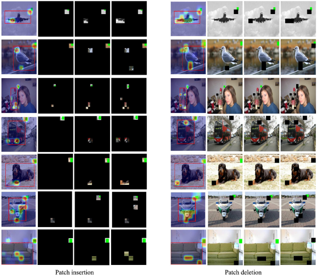
We evaluate the faithfulness of identified regions using the insertion and deletion metrics [8, 32, 33]. In the metrics, the identified regions are ranked in order of importance. In the deletion metric, pixels are gradually removed from the original image, whereas in the insertion metric, pixels are gradually added to an empty image. Then, inferences are performed on these perturbed images, and at each step, a similarity score is calculated to evaluate the similarity between each predicted result and the original result. Here, we evaluate explanations for both bounding box generation and class determination. Following [33], we use Eq. 3 as the similarity score. Finally, we obtain the area under the curve (AUC) from these similarity scores to evaluate the faithfulness of explanations. In the AUC, a higher insertion metric and a lower deletion metric are preferable, indicating that important regions are identified in the initial steps, demonstrating high faithfulness. we also use over-all metric [58], which is the difference between the insertion and deletion metrics, to comprehensively evaluate the insertion and deletion results.

Table 1 summarizes the results of the insertion, deletion, and over-all metrics, showing the average AUC for 1,000 detected instances with a predicted class score $>0.7$ . In the proposed method, the results for the insertion and deletion metrics are generated through patch insertion and patch deletion, respectively. The proposed method with $r=1$ already outperforms existing methods in all metrics except for the insertion metric of Faster R-CNN on PASCAL VOC. Increasing $r$ improves performance, with $r=3$ achieving the best in the over-all metric for all detectors and datasets. These results indicate that the proposed method accurately identifies important regions by considering interactions and Shapley values among many patches.

4.2 Qualitative analysis of visualizations

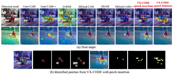
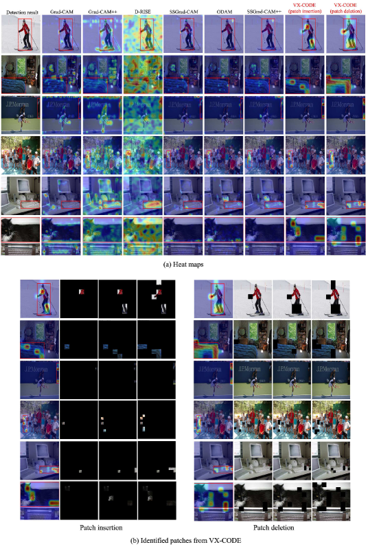
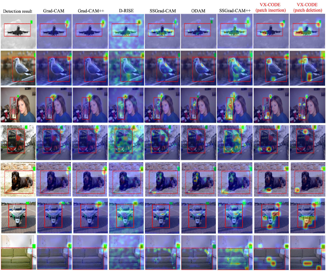
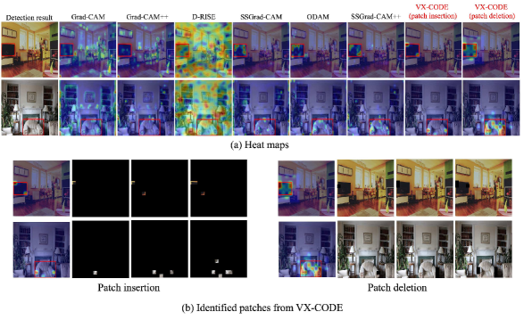
Figure 3 shows the explanations generated by each method for the detections from DETR. As the first row of Fig. 3 shows, the proposed method identifies several features of a car, such as the body, windshield, and shovel. These features collectively influence the detection. The others highlight irrelevant regions or focus solely on the single feature of the shovel. As the second row of Fig. 3 shows, VX-CODE with patch insertion identifies not only the features of the surfboard itself but also those of the sea in the background, indicating that these features collectively contribute to the detection. On the other hand, the others focus only on the surfboard and exhibit low sensitivity to the background. These results suggest an advantage of the proposed method, which considers the collective contributions of multiple patches. Interestingly, VX-CODE with patch deletion focuses only on the surfboard, which differs from the result with patch insertion. This is because patch deletion selects patches to reduce the class score in Eq. 3, thereby prioritizing the elimination of instance features. This is advantageous for object localization. We provide additional visualization results in Sec. C.2.

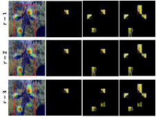
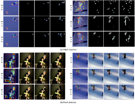
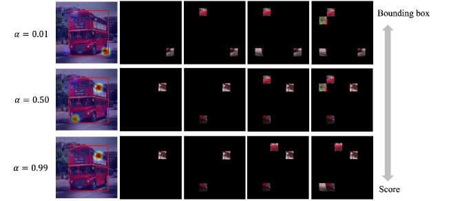
We qualitatively evaluate the effects of increasing $r$ , the number of patches that are inserted or deleted at each step. Figure 4 shows the effect of $r$ on patch identification. For $r=1$ and $r=2$ , very similar regions are selected, such as the neck, forehead, and ears. For $r=3$ , the nose is also identified, which reflects the effect of considering the collective contributions of a larger set of patches (features). Additional visualization results, when $r$ is changed, are provided in Sec. C.3.

Table 2: Ablation study evaluating the effects of patch selection (PS) and step restriction (SR) with

r=2

. The check mark

\checkmark

denotes the inclusion of each module. We show results of insertion (Ins), deletion (Del), over-all (OA) metrics, and explanation generation time per instance (Time), based on 50 instances detected by DETR on MS-COCO. The best values are indicated in bold.

PS	SR	Ins $\uparrow$	Del $\downarrow$	OA $\uparrow$	Time [s] $\downarrow$
		.917	.057	.860	768.13
✓		.917	.059	.858	287.61
	✓	.922	.056	.866	281.78
✓	✓	.921	.058	.863	96.25

4.3 Analysis of patch selection and step restriction

We reduce computational costs using the patch selection and step restriction (see Sec. 3.2.3) when $r\geq 2$ . Table LABEL:tab:effect_a summarizes the effects of these modules with $r=2$ , where each result is computed for 50 instances detected by DETR on MS-COCO, measured on an NVIDIA RTX A6000. As shown in LABEL:tab:effect_a, without patch selection and step restriction, the generation time is substantial. In contrast, incorporating them leads to a significant reduction in generation time, with slight decreases in the insertion and deletion metrics. Interestingly, applying step restriction improves accuracy. This phenomenon indicates that informative patches are selected in the initial steps, making it less beneficial to identify patches with combinations in the later steps.

Table 3: Results of AUC in insertion (Ins), deletion (Del), and over-all (OA) metrics. In VX-CODE, we set

r=1

. Each result is computed for 50 detection instances of the aeroplane class. The best values are indicated in bold.

Metric	Ins $\uparrow$	Del $\downarrow$	OA $\uparrow$
Grad-CAM [40]	.517	.026	.491
Grad-CAM++ [8]	.658	.016	.642
D-RISE [33]	.680	.014	.666
SSGrad-CAM [55]	.649	.053	.596
ODAM [61]	.400	.089	.311
SSGrad-CAM++ [54]	.796	.044	.752
VX-CODE	.891	.034	.857

4.4 Analysis for bias model

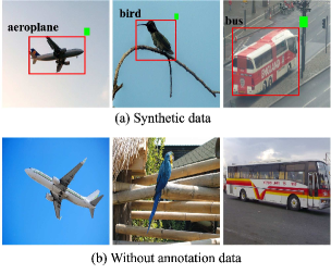
Object detectors sometimes detect instances by considering features outside the bounding box. To analyze the explanations for such cases, we build a model that detects instances by considering features outside the bounding box and evaluates the explanations for its detected results. Specifically, we train DETR on synthetic data set for the seven classes of PASCAL VOC, including aeroplane, bird, bottle, bus, dog, motorbike, and sofa. This synthetic data places a square marker in the upper right corner outside the bounding box (see Fig. 5) for 70% of the instances corresponding to each class. For the remaining 30%, no marker is placed, and the annotations (bounding box and class label) are removed. DETR trained on this data becomes a biased model that, when detecting an aeroplane for example, considers features of both the aeroplane and the marker outside the bounding box. Therefore, reasonable explanations should take both into account. The details of the synthetic data set and the trained model are provided in Sec. C.4.

Figure 5 shows the visualizations generated by each method. Grad-CAM++ and D-RISE highlight only the marker, and SSGrad-CAM++ highlights the entire feature. In contrast, the proposed method successfully identified patches containing features of the airplane and the marker in the early steps. Table 3 shows results in the deletion, insertion, and over-all metrics for the aeroplane class. These results are calculated for 50 detected instances. The proposed method outperforms existing methods, particularly in the insertion metric, where the similarity score improves when both the features of the instance itself and the marker are captured. As shown in Fig. 5, the proposed method efficiently identified these two regions, leading to such results. Interestingly, D-RISE and Grad-CAM++ slightly outperform the proposed method in the deletion metric. The similarity score in the deletion metric decreases considerably if either the instance or the marker is identified. As shown in Fig. 5, D-RISE and Grad-CAM++ tend to strongly highlight only the marker, which contributes to their better performance on this metric. However, these methods fail to capture the instance features, leading to poor performance in the insertion metric. These results indicate that the proposed method provides explanations that consider the influence of both the instance’s and the marker’s features on detection. Additional results are provided in Sec. C.4.

Table 4: Results of AUC for insertion (Ins), deletion (Del), and over-all (OA) metrics. In VX-CODE, we set

r=1

. Each result is computed over 1,000 detection instances with a predicted class score above

0.7

from DETR on MS-COCO. The best values are indicated in bold.

Metric	Ins $\uparrow$	Del $\downarrow$	OA $\uparrow$
Grad-CAM [40]	.799	.474	.325
Grad-CAM++ [8]	.729	.521	.208
D-RISE [33]	.881	.397	.484
SSGrad-CAM [55]	.884	.400	.484
ODAM [61]	.885	.383	502
SSGrad-CAM++ [54]	.864	.401	.463
VX-CODE	.926	.238	.688

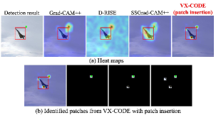
4.5 Analysis for bounding box explanations

We evaluate explanations for bounding box generation. In this experiment, to generate explanations solely for the bounding boxes, we set the following reward function for VX-CODE and D-RISE as a variant of Eq. 3.

\displaystyle f(\mathcal{D}(x);B^{\mathrm{t}})=\underset{B\in\mathcal{D}(x)}{\operatorname{max}}\mathrm{IoU}(B^{\mathrm{t}},B),

(12)

where $\mathcal{D}$ is the object detector, $B^{\mathrm{t}}$ is the target bounding box, and $\mathrm{IoU}(B^{\mathrm{t}},B)$ denotes the IoU between the proposal bounding box $B$ and $B^{\mathrm{t}}$ . For methods utilizing gradients (Grad-CAM, Grad-CAM++, SSGrad-CAM, ODAM, and SSGrad-CAM++), we first generate the heat maps for each bounding box coordinate in $\{x_{1},y_{1},x_{2},y_{2}\}$ following [61]. Then, we obtain the heat map $H_{\mathrm{box}}$ by normalizing these heat maps and summing them together, as follows:

\displaystyle H_{\mathrm{box}}=\sum_{i\in\{x_{1},y_{1},x_{2},y_{2}\}}\frac{H_{i}}{\max(H_{i})},

(13)

where $H_{i}\in\mathbb{R}^{H\times W}$ is the heat map for each bounding box coordinate on a feature map of size $H\times W$ , and $\max(\,\cdot\,)$ calculates the maximum value of a matrix.

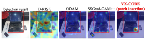
Table 4 shows the results of insertion, deletion, and overall metrics, based on 1,000 instances from the results of DETR on MS-COCO. Here, we use Eq. 12 as the similarity score calculated at each step. The proposed method outperforms the others, demonstrating its ability to accurately identify the important regions for the bounding box generation. Figure 6 compares the visualization results. Generally, the size of a bounding box is determined by several points (at least two). Therefore, considering their collective contributions is important. As shown in Fig. 6, D-RISE, which uses the same reward function, and methods utilizing gradients such as ODAM and SSGrad-CAM++ generate noisy results or highlight irrelevant regions. On the other hand, the proposed method accurately identifies important regions by considering such collective contributions. Additional results are provided in Sec. C.5.

5 Conclusion

In this study, we propose VX-CODE, a visual explanation for object detectors that considers the collective contributions of multiple patches (features). VX-CODE efficiently computes interactions between arbitrary patches and calculates Shapley values for each patch combination. Additionally, we introduce an approach to effectively reduce computational costs as the number of patch combinations increases. Quantitative and qualitative experiments, including benchmark testing, bias models, and bounding box generation, confirm that VX-CODE more accurately identifies important regions compared to existing methods. These findings suggest that the importance of considering collective feature contributions for a deeper understanding of object detector behavior.

Acknowledgments

This work was supported by JSPS KAKENHI Grant Number 23K24914 and JP22K17962.

References

Adebayo et al. [2018] Julius Adebayo, Justin Gilmer, Michael Muelly, Ian Goodfellow, Moritz Hardt, and Been Kim. Sanity checks for saliency maps. In Advances in Neural Information Processing Systems (NeurIPS), 2018.
Ahmed et al. [2024] Ammar Ahmed, Ali Shariq Imran, Abdul Manaf, Zenun Kastrati, and Sher Muhammad Daudpota. Enhancing wrist abnormality detection with yolo: Analysis of state-of-the-art single-stage detection models. Biomedical Signal Processing and Control, 93:106144, 2024.
Bach et al. [2015] Sebastian Bach, Alexander Binder, Grégoire Montavon, Frederick Klauschen, Klaus-Robert Müller, and Wojciech Samek. On pixel-wise explanations for non-linear classifier decisions by layer-wise relevance propagation. PLOS ONE, 10(7):1–46, 2015.
Blücher et al. [2022] Stefan Blücher, Johanna Vielhaben, and Nils Strodthoff. Preddiff: Explanations and interactions from conditional expectations. Artificial Intelligence, 312:103774, 2022.
Bochkovskiy et al. [2020] Alexey Bochkovskiy, Chien-Yao Wang, and H. Liao. Yolov4: Optimal speed and accuracy of object detection. ArXiv, abs/2004.10934, 2020.
Bora et al. [2024] Revoti Prasad Bora, Philipp Terhörst, Raymond Veldhuis, Raghavendra Ramachandra, and Kiran Raja. Slice: Stabilized lime for consistent explanations for image classification. In Proceedings of the IEEE Conference on Computer Vision and Pattern Recognition (CVPR), pages 10988–10996, 2024.
Carion et al. [2020] Nicolas Carion, Francisco Massa, Gabriel Synnaeve, Nicolas Usunier, Alexander Kirillov, and Sergey Zagoruyko. End-to-end object detection with transformers. In Proceedings of the European Conference on Computer Vision (ECCV), page 213–229, 2020.
Chattopadhay et al. [2018] Aditya Chattopadhay, Anirban Sarkar, Prantik Howlader, and Vineeth N Balasubramanian. Grad-cam++: Generalized gradient-based visual explanations for deep convolutional networks. In IEEE Winter Conference on Applications of Computer Vision (WACV), pages 839–847, 2018.
Desai and Ramaswamy [2020] Saurabh Desai and Harish G. Ramaswamy. Ablation-cam: Visual explanations for deep convolutional network via gradient-free localization. In IEEE Winter Conference on Applications of Computer Vision (WACV), pages 972–980, 2020.
Dreyer et al. [2023a] Maximilian Dreyer, Reduan Achtibat, Thomas Wiegand, Wojciech Samek, and Sebastian Lapuschkin. Revealing hidden context bias in segmentation and object detection through concept-specific explanations. In Proceedings of the IEEE Conference on Computer Vision and Pattern Recognition (CVPR) Workshops, pages 3829–3839, 2023a.
Dreyer et al. [2023b] Maximilian Dreyer, Reduan Achtibat, Thomas Wiegand, Wojciech Samek, and Sebastian Lapuschkin. Revealing hidden context bias in segmentation and object detection through concept-specific explanations. In Proceedings of the IEEE Conference on Computer Vision and Pattern Recognition (CVPR) Workshops, pages 3829–3839, 2023b.
Everingham et al. [2010] Mark Everingham, Luc Van Gool, Christopher K. I. Williams, John M. Winn, and Andrew Zisserman. The pascal visual object classes (voc) challenge. Int. J. Comput. Vis., 88(2):303–338, 2010.
Fu et al. [2020] Ruigang Fu, Qingyong Hu, Xiaohu Dong, Yulan Guo, Yinghui Gao, and Biao Li. Axiom-based grad-cam: Towards accurate visualization and explanation of cnns. In British Machine Vision Conference (BMVC), 2020.
Girshick [2015] Ross Girshick. Fast r-cnn. In Proceedings of the IEEE International Conference on Computer Vision (ICCV), pages 1440–1448, 2015.
Grabisch and Roubens [1999] Michel Grabisch and Marc Roubens. “an axiomatic approach to the concept of interaction among players in cooperative games”. International Journal of Game Theory, 28:547–565, 1999.
Gu et al. [2018] Jindong Gu, Yinchong Yang, and Volker Tresp. Understanding individual decisions of cnns via contrastive backpropagation. In Asian Conference on Computer Vision (ACCV), pages 119–134, 2018.
Gwon and Howell [2023] Chul Gwon and Steven C. Howell. Odsmoothgrad: Generating saliency maps for object detectors. In Proceedings of the IEEE Conference on Computer Vision and Pattern Recognition (CVPR) Workshops, pages 3685–3689, 2023.
He et al. [2016] Kaiming He, Xiangyu Zhang, Shaoqing Ren, and Jian Sun. Deep residual learning for image recognition. In Proceedings of the IEEE Conference on Computer Vision and Pattern Recognition (CVPR), pages 770–778, 2016.
Jethani et al. [2022] Neil Jethani, Mukund Sudarshan, Ian Connick Covert, Su-In Lee, and Rajesh Ranganath. FastSHAP: Real-time shapley value estimation. In International Conference on Learning Representations (ICRL), 2022.
Jiang et al. [2024] Mingqi Jiang, Saeed Khorram, and Li Fuxin. Comparing the decision-making mechanisms by transformers and cnns via explanation methods. In Proceedings of the IEEE Conference on Computer Vision and Pattern Recognition (CVPR), pages 9546–9555, 2024.
Jung and Oh [2021] Hyungsik Jung and Youngrock Oh. Towards better explanations of class activation mapping. In IEEE International Conference on Computer Vision (ICCV), pages 1316–1324, 2021.
Khan et al. [2023] Abdul Hannan Khan, Mohammed Shariq Nawaz, and Andreas Dengel. Localized semantic feature mixers for efficient pedestrian detection in autonomous driving. In Proceedings of the IEEE Conference on Computer Vision and Pattern Recognition (CVPR), pages 5476–5485, 2023.
Kuroki and Yamasaki [2024a] Michihiro Kuroki and Toshihiko Yamasaki. Bsed: Baseline shapley-based explainable detector. IEEE Access, 12:57959–57973, 2024a.
Kuroki and Yamasaki [2024b] Michihiro Kuroki and Toshihiko Yamasaki. Fast explanation using shapley value for object detection. IEEE Access, 12:31047–31054, 2024b.
Lin et al. [2014] Tsung-Yi Lin, Michael Maire, Serge Belongie, Lubomir Bourdev, Ross Girshick, James Hays, Pietro Perona, Deva Ramanan, C. Lawrence Zitnick, and Piotr Dollár. Microsoft coco: Common objects in context, 2014.
Lin et al. [2017a] Tsung-Yi Lin, Piotr Dollár, Ross Girshick, Kaiming He, Bharath Hariharan, and Serge Belongie. Feature pyramid networks for object detection. In Proceedings of the IEEE Conference on Computer Vision and Pattern Recognition (CVPR), pages 936–944, 2017a.
Lin et al. [2017b] Tsung-Yi Lin, Priya Goyal, Ross Girshick, Kaiming He, and Piotr Dollár. Focal loss for dense object detection. In IEEE International Conference on Computer Vision (ICCV), pages 2999–3007, 2017b.
Liu et al. [2016] Wei Liu, Dragomir Anguelov, Dumitru Erhan, Christian Szegedy, Scott E. Reed, Cheng-Yang Fu, and Alexander C. Berg. SSD: Single shot multibox detector. In Proceedings of the European Conference on Computer Vision (ECCV), pages 21–37, 2016.
Lundberg and Lee [2017] Scott M. Lundberg and Su-In Lee. A unified approach to interpreting model predictions. In Advances in Neural Information Processing Systems (NeurIPS), page 4768–4777, 2017.
Nguyen et al. [2022] Ethan H. Nguyen, Haichun Yang, Ruining Deng, Yuzhe Lu, Zheyu Zhu, Joseph T. Roland, Le Lu, Bennett A. Landman, Agnes B. Fogo, and Yuankai Huo. Circle representation for medical object detection. IEEE Transactions on Medical Imaging, 41(3):746–754, 2022.
Paszke et al. [2017] Adam Paszke, Sam Gross, Soumith Chintala, Gregory Chanan, Edward Yang, Zachary DeVito, Zeming Lin, Alban Desmaison, Luca Antiga, and Adam Lerer. Automatic differentiation in pytorch. In Advances in Neural Information Processing Systems (NeurIPS) Workshop on Autodiff, 2017.
Petsiuk et al. [2018] Vitali Petsiuk, Abir Das, and Kate Saenko. Rise: Randomized input sampling for explanation of black-box models. In British Machine Vision Conference (BMVC), page 151, 2018.
Petsiuk et al. [2021] Vitali Petsiuk, Rajiv Jain, Varun Manjunatha, Vlad I. Morariu, Ashutosh Mehra, Vicente Ordonez, and Kate Saenko. Black-box explanation of object detectors via saliency maps. In Proceedings of the IEEE Conference on Computer Vision and Pattern Recognition (CVPR), pages 11443–11452, 2021.
Raghu et al. [2021] Maithra Raghu, Thomas Unterthiner, Simon Kornblith, Chiyuan Zhang, and Alexey Dosovitskiy. Do vision transformers see like convolutional neural networks? In Advances in Neural Information Processing Systems (NeurIPS), pages 12116–12128, 2021.
Redmon and Farhadi [2017] Joseph Redmon and Ali Farhadi. Yolo9000: Better, faster, stronger. In Proceedings of the IEEE Conference on Computer Vision and Pattern Recognition (CVPR), pages 6517–6525, 2017.
Redmon and Farhadi [2018] Joseph Redmon and Ali Farhadi. YOLOv3: An Incremental Improvement. arXiv.org, pages 1–6, 2018.
Redmon et al. [2016] Joseph Redmon, Santosh Divvala, Ross Girshick, and Ali Farhadi. You only look once: Unified, real-time object detection. In Proceedings of the IEEE Conference on Computer Vision and Pattern Recognition (CVPR), pages 779–788, 2016.
Ren et al. [2015] Shaoqing Ren, Kaiming He, Ross B. Girshick, and Jian Sun. Faster r-cnn: Towards real-time object detection with region proposal networks. In Advances in Neural Information Processing Systems (NeurIPS), pages 91–99, 2015.
Ribeiro et al. [2016] Marco Tulio Ribeiro, Sameer Singh, and Carlos Guestrin. ”why should I trust you?”: Explaining the predictions of any classifier. In Proceedings of the 22nd ACM SIGKDD International Conference on Knowledge Discovery and Data Mining, pages 1135–1144, 2016.
Selvaraju et al. [2017] Ramprasaath R. Selvaraju, Michael Cogswell, Abhishek Das, Ramakrishna Vedantam, Devi Parikh, and Dhruv Batra. Grad-cam: Visual explanations from deep networks via gradient-based localization. In Proceedings of the IEEE International Conference on Computer Vision (ICCV), pages 618–626, 2017.
Shapley [1953] Lloyd S Shapley. A value for n-person games. In Contributions to the Theory of Games II, pages 307–317. 1953.
Shrikumar et al. [2017] Avanti Shrikumar, Peyton Greenside, and Anshul Kundaje. Learning important features through propagating activation differences. In Proceedings of the International Conference on Machine Learning (ICML), page 3145–3153, 2017.
Simonyan et al. [2013] Karen Simonyan, Andrea Vedaldi, and Andrew Zisserman. Deep inside convolutional networks: Visualising image classification models and saliency maps. CoRR, abs/1312.6034, 2013.
Smilkov et al. [2017] Daniel Smilkov, Nikhil Thorat, Been Kim, Fernanda B. Viégas, and Martin Wattenberg. Smoothgrad: removing noise by adding noise. CoRR, abs/1706.03825, 2017.
Springenberg et al. [2015] Jost Tobias Springenberg, Alexey Dosovitskiy, Thomas Brox, and Martin Riedmiller. Striving for simplicity: The all convolutional net. In International Conference on Learning Representations (ICLR) workshop track, 2015.
Sumiyasu et al. [2024] Kosuke Sumiyasu, Kazuhiko Kawamoto, and Hiroshi Kera. Identifying important group of pixels using interactions. In Proceedings of the IEEE Conference on Computer Vision and Pattern Recognition (CVPR), pages 6017–6026, 2024.
Sundararajan and Najmi [2020] Mukund Sundararajan and Amir Najmi. The many shapley values for model explanation. In Proceedings of the International Conference on Machine Learning (ICML), 2020.
Sundararajan et al. [2017] Mukund Sundararajan, Ankur Taly, and Qiqi Yan. Axiomatic attribution for deep networks. In International Conference on Machine Learning, 2017.
Tian et al. [2019] Zhi Tian, Chunhua Shen, Hao Chen, and Tong He. FCOS: Fully convolutional one-stage object detection. In Proceedings of the IEEE International Conference on Computer Vision (ICCV), pages 9626–9635, 2019.
Truong et al. [2024] Van Binh Truong, Truong Thanh Hung Nguyen, Vo Thanh Khang Nguyen, Quoc Khanh Nguyen, and Quoc Hung Cao. Towards better explanations for object detection. In Asian Conference on Computer Vision (ACCV), pages 1385–1400, 2024.
Tuli et al. [2021] Shikhar Tuli, Ishita Dasgupta, Erin Grant, and Thomas L. Griffiths. Are convolutional neural networks or transformers more like human vision? ArXiv, abs/2105.07197, 2021.
Wang et al. [2020] Haofan Wang, Zifan Wang, Mengnan Du, Fan Yang, Zijian Zhang, Sirui Ding, Piotr Mardziel, and Xia Hu. Score-cam: Score-weighted visual explanations for convolutional neural networks. In Proceedings of the IEEE Conference on Computer Vision and Pattern Recognition (CVPR) Workshops, pages 111–119, 2020.
Wu et al. [2019] Yuxin Wu, Alexander Kirillov, Francisco Massa, Wan-Yen Lo, and Ross Girshick. Detectron2. https://github.com/facebookresearch/detectron2, 2019.
Yamauchi [2024] Toshinori Yamauchi. Spatial sensitive grad-cam++: Improved visual explanation for object detectors via weighted combination of gradient map. In Proceedings of the IEEE Conference on Computer Vision and Pattern Recognition (CVPR) Workshops, pages 8164–8168, 2024.
Yamauchi and Ishikawa [2022] Toshinori Yamauchi and Masayoshi Ishikawa. Spatial sensitive grad-cam: Visual explanations for object detection by incorporating spatial sensitivity. In IEEE International Conference on Image Processing (ICIP), pages 256–260, 2022.
Zeiler and Fergus [2013] Matthew D. Zeiler and Rob Fergus. Visualizing and understanding convolutional networks. CoRR, abs/1311.2901, 2013.
Zhang et al. [2018a] Jianming Zhang, Zhe L. Lin, Jonathan Brandt, Xiaohui Shen, and Stan Sclaroff. Top-down neural attention by excitation backprop. International Journal of Computer Vision, 126:1084–1102, 2018a.
Zhang et al. [2021] Qinglong Zhang, Lu Rao, and Yubin Yang. Group-cam: Group score-weighted visual explanations for deep convolutional networks, 2021.
Zhang et al. [2018b] Shifeng Zhang, Longyin Wen, Xiao Bian, Zhen Lei, and Stan Z. Li. Single-shot refinement neural network for object detection. In Proceedings of the IEEE Conference on Computer Vision and Pattern Recognition (CVPR), 2018b.
Zhang et al. [2024] Yi Zhang, Wang Zeng, Sheng Jin, Chen Qian, Ping Luo, and Wentao Liu. When pedestrian detection meets multi-modal learning: Generalist model and benchmark dataset, 2024.
Zhao et al. [2024] C. Zhao, J. H. Hsiao, and A. B. Chan. Gradient-based instance-specific visual explanations for object specification and object discrimination. IEEE Transactions on Pattern Analysis & Machine Intelligence, 46(09):5967–5985, 2024.
Zheng et al. [2022] Quan Zheng, Ziwei Wang, Jie Zhou, and Jiwen Lu. Shap-cam: Visual explanations for convolutional neural networks based on shapley value. In Proceedings of the European Conference on Computer Vision (ECCV), page 459–474, 2022.
Zhou et al. [2016] Bolei Zhou, Aditya Khosla, Agata Lapedriza, Aude Oliva, and Antonio Torralba. Learning deep features for discriminative localization. In Proceedings of the IEEE Conference on Computer Vision and Pattern Recognition (CVPR), 2016.
Zhu et al. [2021] Xizhou Zhu, Weijie Su, Lewei Lu, Bin Li, Xiaogang Wang, and Jifeng Dai. Deformable DETR: deformable transformers for end-to-end object detection. In International Conference on Learning Representations (ICLR), 2021.

\thetitle

Supplementary Material

Appendix A Visual explanations for classification

In the main paper, we omitted detailed discussions of related work due to space constraints; here, we provide a more comprehensive review.

Various visual explanation methods have been proposed for image classification models [1, 39, 40, 8, 52, 32, 13, 62, 46]. Generally, these methods can be broadly classified into three categories: gradient-based, class-activation-based (CAM-based), and perturbation-based.

Gradient-based methods generate a saliency map by calculating the gradient of each pixel in the input image with respect to the model’s output score, visualizing the important regions [43, 56, 45, 3, 44, 57, 48, 42, 16]. For example, LRP [3] computes pixel-wise feature attributions by propagating relevance from the output layer to the input layer. CPR [16] extends LRP by emphasizing the relevance originating from the target class, calculating the disparity between the relevance from the target class and the average relevance from other classes.

CAM-based methods calculate the weights representing the importance of each channel in the feature maps, and visualize important regions by computing the weighted sum of these weights and the feature maps [63, 40, 8, 52, 13, 9, 21, 62]. CAM [63] incorporates global average pooling into the CNN and generates a heat map that highlights important regions. Grad-CAM [40] generalizes CAM, making it possible to incorporate it into any CNN. Grad-CAM++ [8] improves upon Grad-CAM by incorporating pixel-level weighting, thereby enhancing the quality of the heat map. Other methods that more accurately compute the weights representing the importance of each channel have been proposed [52, 13, 9, 62].

Perturbation-based methods identify important regions by introducing perturbations to the input image and quantifying the changes in the output [39, 32, 29, 47, 4, 19, 46]. LIME [39, 6] occludes by using super-pixel to compute the importance score. RISE [32] visualizes important regions by applying random masks to the input image and analyzing the output results generated from the masked images. SHAP [29] distributes confidence scores to contributions by utilizing Shapley values from game theory. Methods that consider interactions [15] in addition to Shapley values have also been proposed [4, 46]. PredDIFF [4] is a method that measures changes in predictions by marginalizing features from a probabilistic perspective. This paper clarifies the relationship between PredDIFF and Shapley values, and introduces a new measurement method that takes interactions into account. MoXI [46] utilizes a technique to approximate Shapley values and interactions to identify important regions for classification models. Our proposed VX-CODE utilizes and expands this technique to provide explanations for object detectors.

Algorithm 1 Process of patch insertion

0: Reward function

f

,index set

N

of patches, the number of patches

r\in\{1,\ldots,|N|\}

inserted at each step, patch selection parameter

L\in\{1,\ldots,|N|\}

, step restriction parameter

\gamma\in[0,1]

0: Sequence of subsets

S_{1},\ldots,S_{E}\subseteq N

S_{k}\leftarrow\{\}

for all

k=0,\ldots,E

T=N

k=1

3: while

|T|\neq 0

4: if

|T|<r

then

r\leftarrow|T|

6: end if

7: if

r\geq 2

and

|S_{k-1}|\leq\gamma|N|

then

8: # Require

|N\setminus S_{k-1}|

forward process.

P^{L}_{k}\leftarrow\underset{P\subseteq N\setminus S_{k-1}}{\operatorname{arg\,max}}\;\sum_{b\in P}f(S_{k-1}\cup\{b\})

10: # Require

{}_{L}C_{r}

forward process.

11:

B^{r}_{k}\leftarrow\underset{B^{r}\subseteq P^{L}_{k}}{\operatorname{arg\,max}}\;f(S_{k-1}\cup B^{r})

12:

S_{k}\leftarrow S_{k-1}\cup B^{r}_{k}

13:

T\leftarrow T\setminus B^{r}_{k}

14:

k\leftarrow k+1

15: else

16: # Require

|N\setminus S_{k-1}|

forward process.

17:

b_{k}\leftarrow\underset{b\in N\setminus S_{k-1}}{\operatorname{arg\,max}}\;f(S_{k-1}\cup\{b_{k}\})

18:

S_{k}\leftarrow S_{k-1}\cup\{b_{k}\}

19:

T\leftarrow T\setminus\{b_{k}\}

20:

k\leftarrow k+1

21: end if

22: end while

23: return

S_{1},\ldots,S_{E}

Algorithm 2 Process of patch deletion

0: Reward function

f

, index set

N

of patches, the number of patches

r\in\{1,\ldots,|N|\}

inserted at each step, patch selection parameter

L\in\{1,\ldots,|N|\}

,step restriction parameter

\gamma\in[0,1]

0: Sequence of subsets

S_{1},\ldots,S_{E}\subseteq N

S_{k}\leftarrow\{\}

for all

k=0,\ldots,E

T=N

k=1

3: while

|T|\neq 0

4: if

|T|<r

then

r\leftarrow|T|

6: end if

7: if

r\geq 2

and

|S_{k-1}|\leq\gamma|N|

then

8: # Require

|N\setminus S_{k-1}|

forward process.

P^{L}_{k}\leftarrow\underset{P\subseteq N\setminus S_{k-1}}{\operatorname{arg\,max}}\;\sum_{b\in P}-f(N\setminus(S_{k-1}\cup\{b\}))

10: # Require

{}_{L}C_{r}

forward process.

11:

B^{r}_{k}\leftarrow\underset{B^{r}\subseteq P^{L}_{k}}{\operatorname{arg\,min}}\;f(N\setminus(S_{k-1}\cup B^{r}))

12:

S_{k}\leftarrow S_{k-1}\cup B^{r}_{k}

13:

T\leftarrow T\setminus B^{r}_{k}

14:

k\leftarrow k+1

15: else

16: # Require

|N\setminus S_{k-1}|

forward process.

17:

b_{k}\leftarrow\underset{b\in N\setminus S_{k-1}}{\operatorname{arg\,min}}\;f(N\setminus(S_{k-1}\cup\{b_{k}\}))

18:

S_{k}\leftarrow S_{k-1}\cup\{b_{k}\}

19:

T\leftarrow T\setminus\{b_{k}\}

20:

k\leftarrow k+1

21: end if

22: end while

23: return

S_{1},\ldots,S_{E}

Appendix B Detailed of the proposed method

In this section, we provide details of the proposed method that are not included in the main paper.

B.1 Details of the algorithm

We summarize the algorithm of VX-CODE. The processes of patch insertion and patch deletion are shown in Algorithm 1 and Algorithm 2, respectively. As shown in these algorithms, VX-CODE identifies $r$ patches or a single patch at each step based on the value of the reward function, using a simple greedy algorithm.

B.2 Specific example of patch insertion

We provide specific examples for cases with $r=1$ and $r=2$ in patch insertion described in Sec. 3.2.2.

B.2.1 Case with $r=1$

For step $k=1$ , from Eq. 5, only the highest Shapley value $\phi(\{b_{1}\}|\{\{b_{1}\}\})$ becomes the optimal set $S_{1}=\{b_{1}\}$ .

For $k\geq 2$ , we find $b_{k}$ that maximizes $f(S_{k-1}\cup\{b_{k}\})$ . From Eq. 9, this is formulated as follows:

$\displaystyle b_{k}$	$\displaystyle=\underset{b\in N\setminus{S_{k-1}}}{\operatorname{arg\,max}}\;f(\{S_{k-1},b\})-f(\emptyset)$
	$\displaystyle=\underset{b\in N\setminus{S_{k-1}}}{\operatorname{arg\,max}}\;\phi^{\mathrm{sc}}(\{S_{k-1},b\})$
	$\displaystyle=\underset{b\in N\setminus{S_{k-1}}}{\operatorname{arg\,max}}\;I_{2}^{\mathrm{sc}}(\{S_{k-1},b\})$
	$\displaystyle\quad\quad\quad\quad+\sum_{r^{\prime}=1}^{1}\left(\sum_{c\in\mathcal{P}_{r^{\prime}}(S_{k-1}\cup\{b\})}\phi^{\mathrm{sc}}(c)\right)$
	$\displaystyle=\underset{b\in N\setminus{S_{k-1}}}{\operatorname{arg\,max}}\;I_{2}^{\mathrm{sc}}(\{S_{k-1},b\})+\phi^{\mathrm{sc}}(\{b\})+\phi^{\mathrm{sc}}(S_{k-1})$
	$\displaystyle=\underset{b\in N\setminus{S_{k-1}}}{\operatorname{arg\,max}}\;I_{2}^{\mathrm{sc}}(\{S_{k-1},b\})+\phi^{\mathrm{sc}}(\{b\}).$	(14)

Therefore, this selection considers interactions between $S_{k-1}$ and $b_{k}$ , as well as the Shapley values of $b_{k}$ in the self-context.

B.2.2 Case with $r=2$

For $k=1$ , we find $b_{1}$ and $b_{2}$ so that $f(\{b_{1},b_{2}\})$ is maximized. From Eqs. 5 and 3.2.2, this is formulated as follows:

$\displaystyle\{b_{1},b_{2}\}$	$\displaystyle=\underset{\{b^{\prime}_{1},b^{\prime}_{2}\}\subset N}{\operatorname{arg\,max}}\;f(\{b^{\prime}_{1},b^{\prime}_{2}\})-f(\emptyset)$
	$\displaystyle=\underset{\{b^{\prime}_{1},b^{\prime}_{2}\}\subset N}{\operatorname{arg\,max}}\;\phi^{\mathrm{sc}}(\{b^{\prime}_{1},b^{\prime}_{2}\})$
	$\displaystyle=\underset{\{b^{\prime}_{1},b^{\prime}_{2}\}\subset N}{\operatorname{arg\,max}}\;I_{2}^{\mathrm{sc}}(\{b^{\prime}_{1},b^{\prime}_{2}\})$
	$\displaystyle\quad\quad\quad\quad+\sum_{r^{\prime}=1}^{1}\left(\sum_{c\in\mathcal{P}_{r^{\prime}}(\{b^{\prime}_{1},b^{\prime}_{2}\})}\phi^{\mathrm{sc}}(c)\right)$
	$\displaystyle=\underset{\{b^{\prime}_{1},b^{\prime}_{2}\}\subset N}{\operatorname{arg\,max}}\;I_{2}^{\mathrm{sc}}(\{b^{\prime}_{1},b^{\prime}_{2}\})$
	$\displaystyle\quad\quad\quad\quad+\phi^{\mathrm{sc}}(\{b^{\prime}_{1}\})+\phi^{\mathrm{sc}}(\{b^{\prime}_{2}\}).$	(15)

Therefore, this selection considers interactions between $b_{1}$ and $b_{2}$ , as well as their Shapley values in the self-context.

For $k\geq 2$ , we find $b_{2k-1}$ and $b_{2k}$ so that maximizes $f(S_{k-1}\cup\{b_{2k-1},b_{2k}\})$ is maximized. From Eq. 9, this is formulated as follows:

	$\displaystyle\{b_{2k-1},b_{2k}\}$		(16)
	$\displaystyle=\underset{\{b^{\prime}_{2k-1},b^{\prime}_{2k}\}\subseteq N\setminus{S_{k-1}}}{\operatorname{arg\,max}}\;f(\{S_{k-1},b^{\prime}_{2k-1},b^{\prime}_{2k}\})-f(\emptyset)$
	$\displaystyle=\underset{\{b^{\prime}_{2k-1},b^{\prime}_{2k}\}\subseteq N\setminus{S_{k-1}}}{\operatorname{arg\,max}}\phi^{\mathrm{sc}}(\{S_{k-1},b^{\prime}_{2k-1},b^{\prime}_{2k}\})$
	$\displaystyle=\underset{\{b^{\prime}_{2k-1},b^{\prime}_{2k}\}\subseteq N\setminus{S_{k-1}}}{\operatorname{arg\,max}}\;I_{3}^{\mathrm{sc}}(\{S_{k-1},b^{\prime}_{2k-1},b^{\prime}_{2k}\})$
	$\displaystyle\quad\quad\quad\quad+\sum_{r^{\prime}=1}^{2}\left(\sum_{c\in\mathcal{P}_{r^{\prime}}(S_{k-1}\cup\{b^{\prime}_{2k-1},b^{\prime}_{2k}\})}\phi^{\mathrm{sc}}(c)\right)$
	$\displaystyle=\underset{\{b^{\prime}_{2k-1},b^{\prime}_{2k}\}\subseteq N\setminus{S_{k-1}}}{\operatorname{arg\,max}}\;I_{3}^{\mathrm{sc}}(\{S_{k-1},b^{\prime}_{2k-1},b^{\prime}_{2k}\})$
	$\displaystyle\quad\quad\quad\quad+\phi^{\mathrm{sc}}(\{S_{k-1},b^{\prime}_{2k-1}\})+\phi^{\mathrm{sc}}(\{S_{k-1},b^{\prime}_{2k}\})$
	$\displaystyle\quad\quad\quad\quad+\phi^{\mathrm{sc}}(\{b^{\prime}_{2k-1},b^{\prime}_{2k})+\phi^{\mathrm{sc}}(\{b^{\prime}_{2k-1}\})$
	$\displaystyle\quad\quad\quad\quad+\phi^{\mathrm{sc}}(\{b^{\prime}_{2k}\})+\phi^{\mathrm{sc}}(S^{\prime}_{k-1})$
	$\displaystyle=\underset{\{b^{\prime}_{2k-1},b^{\prime}_{2k}\}\subseteq N\setminus{S_{k-1}}}{\operatorname{arg\,max}}\;I_{3}^{\mathrm{sc}}(\{S_{k-1},b^{\prime}_{2k-1},b^{\prime}_{2k}\})$
	$\displaystyle\quad\quad\quad\quad+\phi^{\mathrm{sc}}(\{S_{k-1},b^{\prime}_{2k-1}\})+\phi^{\mathrm{sc}}(\{S_{k-1},b^{\prime}_{2k}\})$
	$\displaystyle\quad\quad\quad\quad+\phi^{\mathrm{sc}}(\{b^{\prime}_{2k-1},b^{\prime}_{2k})+\phi^{\mathrm{sc}}(\{b^{\prime}_{2k-1}\})+\phi^{\mathrm{sc}}(\{b^{\prime}_{2k}\}).$		(17)

Therefore, this selection considers interactions among the three elements $S_{k-1}$ , $b_{2k-1}$ , and $b_{2k}$ , as well as Shapley values derived from each patch combination in self-context.

B.3 Patch deletion

We explain the process of patch deletion. In patch deletion, we address the following problem.

Problem 2

Under the same conditions as those for patch insertion outlined in Problem 1, find a subset $S_{k}\subset N$ such that

\displaystyle S_{k}=\underset{{S\subseteq N,|S|=k}}{\mathrm{arg\,min}}\;f(N\setminus S),

(18)

for $k=1,\ldots,n$ .

Similar to patch insertion, we adopt a greedy approach once again to approximate the solution. Specifically, at each step $k$ , we remove $r\in\{1,\ldots,n\}$ patches and determine the subset that minimize the reward. Here, we utilize the Shapley value which measures the contribution in the absence of a player.

\displaystyle\phi_{\mathrm{d}}(i\mid N)\stackrel{{\scriptstyle\mathrm{def}}}{{=}}\sum_{S\subseteq N,i\in S}P_{\mathrm{d}}(S\setminus\{i\}\mid N)[f(S)-f(S\setminus\{i\})].

(19)

where $P_{\mathrm{d}}(A\mid B)=\frac{(|B|-|A|-1)!|A|!}{|B|!}$ . This Shapley value quantifies the average impact attributable to the removal of player $i$ .

For $k=1$ , the set of patches $B^{r}_{1}=\{b_{1},\ldots,b_{r}\}$ is selected so that $f(N\setminus B^{r}_{1})$ is minimized.

$\displaystyle B^{r}_{1}$	$\displaystyle=\underset{B^{r}\subseteq N}{\operatorname{arg\,min}}\;f(N\setminus B^{r})-f(N)$
	$\displaystyle=\underset{B^{r}\subseteq N}{\operatorname{arg\,max}}\;f(N)-f(N\setminus B^{r})$
	$\displaystyle=\underset{B^{r}\subseteq N}{\operatorname{arg\,max}}\;\phi_{\mathrm{d}}^{\mathrm{fc}}(B^{r}\mid N),$	(20)

where

\displaystyle\phi_{\mathrm{d}}^{\mathrm{fc}}(B^{r}\mid N)\stackrel{{\scriptstyle\mathrm{def}}}{{=}}P_{\mathrm{d}}(N\setminus B^{r}\mid N)[f(N)-f(N\setminus B^{r})].

(21)

In the last equality, we omit $P_{\mathrm{d}}(N\setminus B^{r}_{1}\mid N)$ , as it remains constant regardless of the patch selection. The quantity $\phi_{\mathrm{d}}^{\mathrm{fc}}$ is known as the Shapley value in full-context [46], which is restricted to a specific set $S$ in Eq. 19. Next, similar to patch insertion, we define the interaction in the full context as follows:

	$\displaystyle I_{\mathrm{d},r}^{\mathrm{fc}}(B^{r})\stackrel{{\scriptstyle\mathrm{def}}}{{=}}\phi_{\mathrm{d}}^{\mathrm{fc}}(B^{r}\mid N\setminus B^{r}\cup\{B^{r}\})$
	$\displaystyle\quad\quad\quad\quad-\sum_{r^{\prime}=1}^{r-1}\left(\sum_{c\in\mathcal{P}_{r^{\prime}}(B^{r})}\phi_{\mathrm{d}}^{\mathrm{fc}}(c\mid N\setminus\{B^{r}\setminus c\})\right).$		(22)

Noting that $\phi_{\mathrm{d}}^{\mathrm{fc}}(B^{r}\mid N\setminus B^{r}\cup\{B^{r}\})=\phi_{\mathrm{d}}^{\mathrm{fc}}(B^{r}\mid N)$ , from Eqs. 20 and 22, we get

$\displaystyle B^{r}_{1}$	$\displaystyle=\underset{B^{r}\subseteq N}{\operatorname{arg\,max}}\;\phi_{\mathrm{d}}^{\mathrm{fc}}(B^{r}\mid N)$
	$\displaystyle=\underset{B^{r}\subseteq N}{\operatorname{arg\,max}}\;\underbrace{I_{\mathrm{d},r}^{\mathrm{fc}}(B^{r})}_{\text{Interaction}}$
	$\displaystyle\quad\quad\quad\quad+\underbrace{\sum_{r^{\prime}=1}^{r-1}\left(\sum_{c\in\mathcal{P}_{r^{\prime}}(B^{r})}\phi_{\mathrm{d}}^{\mathrm{fc}}(c\mid N\setminus\{B^{r}\setminus c\})\right)}_{\text{Shapley values}}.$	(23)

Therefore, at step $k=1$ , the selection considers both interactions of the $r$ patches (the first term) and Shapley values of each patch combination (the second term). In the case of $r=1$ , from Eq. 20, the highest Shapley value $\phi_{\mathrm{d}}^{\mathrm{fc}}(\{b_{1}\}\mid N)=n^{-1}[f(N)-f(N\setminus\{b_{1}\}]$ becomes the optimal set.

$\displaystyle B^{r}_{k}$	$\displaystyle=\underset{B^{r}\subseteq N\setminus S_{k-1}}{\operatorname{arg\,min}}\;f(N\setminus\{S_{k-1},B^{r}\})-f(N)$
	$\displaystyle=\underset{B^{r}\subseteq N\setminus S_{k-1}}{\operatorname{arg\,max}}\;f(N)-f(N\setminus\{S_{k-1},B^{r}\})$
	$\displaystyle=\underset{B^{r}\subseteq N\setminus S_{k-1}}{\operatorname{arg\,max}}\;\phi_{\mathrm{d}}^{\mathrm{fc}}(\{S_{k-1},B^{r}\}\mid N)$
	$\displaystyle=\underset{B^{r}\subseteq N\setminus S_{k-1}}{\operatorname{arg\,max}}\;\underbrace{I_{\mathrm{d},r+1}^{\mathrm{fc}}(\{S_{k-1},B^{r}\})}_{\text{Interaction}}$
	$\displaystyle+\underbrace{\sum_{r^{\prime}=1}^{r}\left(\sum_{c\in\mathcal{P}_{r^{\prime}}(S_{k-1}\cup B^{r})}\phi_{\mathrm{d}}^{\mathrm{fc}}(c\mid N\setminus\{S_{k-1}\cup B^{r}\setminus c\})\right)}_{\text{Shapley values}}.$	(24)

where $S_{k-1}$ is regarded as a single patch. Hence, for step $k\geq 2$ , the selection $B^{r}_{k}$ considers interactions between the already identified patch set $S_{k-1}$ and the $r$ patches, resulting in $r+1$ interactions (the first term), as well as Shapley values of each patch combination (the second term).

As described above, similar to patch insertion, patch deletion considers both Shapley values and interactions, and increasing $r$ allows for considering these metrics among a larger number of patches. The over all algorithm is shown in Algorithm 2. Next section, we describe specific examples in patch deletion with $r=1$ and $r=2$ .

B.4 Specific example of patch deletion

We provide specific examples for cases with $r=1$ and $r=2$ in patch deletion described in Sec. B.3.

B.5 Case with $r=1$

For step $k=1$ , from Eq. 20, only the highest Shapley value $\phi_{\mathrm{d}}^{\mathrm{fc}}(\{b_{1}\}|N)=n^{-1}[f(N)-f(N\setminus\{b_{1}\}]$ becomes the optimal set $S_{1}=\{b_{1}\}$ .

For $k\geq 2$ , we find $b_{k}$ that minimizes $f(N\setminus\{S_{k-1},b_{k}\})$ . From Eq. 24, this is formulated as follows:

$\displaystyle b_{k}$	$\displaystyle=\underset{b\subseteq N\setminus S_{k-1}}{\operatorname{arg\,min}}\;f(N\setminus\{S_{k-1},b\})-f(N)$
	$\displaystyle=\underset{b\subseteq N\setminus S_{k-1}}{\operatorname{arg\,max}}\;f(N)-f(N\setminus\{S_{k-1},b\})$
	$\displaystyle=\underset{b\subseteq N\setminus S_{k-1}}{\operatorname{arg\,max}}\;\phi_{\mathrm{d}}^{\mathrm{fc}}(\{S_{k-1},b\}\mid N)$
	$\displaystyle=\underset{b\subseteq N\setminus S_{k-1}}{\operatorname{arg\,max}}\;I_{\mathrm{d},2}^{\mathrm{fc}}(\{S_{k-1},b\})$
	$\displaystyle\quad+\sum_{r^{\prime}=1}^{1}\left(\sum_{c\in\mathcal{P}_{r^{\prime}}(S_{k-1}\cup\{b\})}\phi_{\mathrm{d}}^{\mathrm{fc}}(c\mid N\setminus\{S_{k-1}\cup\{b\}\setminus c\})\right)$
	$\displaystyle=\underset{b\subseteq N\setminus S_{k-1}}{\operatorname{arg\,max}}\;I_{\mathrm{d},2}^{\mathrm{fc}}(\{S_{k-1},b\})$
	$\displaystyle\quad\quad\quad\quad+\phi_{\mathrm{d}}^{\mathrm{fc}}(\{b\}\mid N\setminus S_{k-1})+\phi_{\mathrm{d}}^{\mathrm{fc}}(S_{k-1}\mid N\setminus\{b\}).$	(25)

Therefore, this selection considers interactions between $S_{k-1}$ and $b_{k}$ , as well as Shapley values of $S_{k-1}$ and $b_{k}$ in the full-context.

B.6 Case with $r=2$

For $k=1$ , we find $b_{1}$ and $b_{2}$ so that $f(N\setminus\{b_{1},b_{2}\})$ is minimized. From Eqs. 20 and 23, this is formulated as follows:

$\displaystyle\{b_{1},b_{2}\}$	$\displaystyle=\underset{\{b^{\prime}_{1},b^{\prime}_{2}\}\subset N}{\operatorname{arg\,min}}\;f(N\setminus\{b^{\prime}_{1},b^{\prime}_{2}\})-f(N)$
	$\displaystyle=\underset{\{b^{\prime}_{1},b^{\prime}_{2}\}\subset N}{\operatorname{arg\,max}}\;f(N)-f(N\setminus\{b^{\prime}_{1},b^{\prime}_{2}\})$
	$\displaystyle=\underset{\{b^{\prime}_{1},b^{\prime}_{2}\}\subset N}{\operatorname{arg\,max}}\;\phi_{\mathrm{d}}^{\mathrm{fc}}(\{b^{\prime}_{1},b^{\prime}_{2}\}\mid N)$
	$\displaystyle=\underset{\{b^{\prime}_{1},b^{\prime}_{2}\}\subset N}{\operatorname{arg\,max}}\;I_{\mathrm{d},2}^{\mathrm{fc}}(\{b^{\prime}_{1},b^{\prime}_{2}\})$
	$\displaystyle\quad+\sum_{r^{\prime}=1}^{1}\left(\sum_{c\in\mathcal{P}_{r^{\prime}}(\{b^{{}^{\prime}}_{1},b^{{}^{\prime}}_{2}\})}\phi_{\mathrm{d}}^{\mathrm{fc}}(c\mid N\setminus\{\{b^{\prime}_{1},b^{\prime}_{2}\}\setminus c\})\right)$
	$\displaystyle=\underset{\{b^{\prime}_{1},b^{\prime}_{2}\}\subset N}{\operatorname{arg\,max}}\;I_{\mathrm{d},2}^{\mathrm{fc}}(\{b^{\prime}_{1},b^{\prime}_{2}\})$
	$\displaystyle\quad+\phi_{\mathrm{d}}^{\mathrm{fc}}(\{b^{\prime}_{1}\}\mid N\setminus\{b^{\prime}_{2}\})+\phi_{\mathrm{d}}^{\mathrm{fc}}(\{b^{\prime}_{2}\}\mid N\setminus\{b^{\prime}_{1}\}).$	(26)

Therefore, this selection considers interactions between $b_{1}$ and $b_{2}$ , as well as their Shapley values in the full-context.

For $k\geq 2$ , we find $b_{2k-1}$ and $b_{2k}$ so that $f(N\setminus\{S_{k-1},b_{2k-1},b_{2k}\})$ is minimized. From Eq. 24, this is formulated as follows:

	$\displaystyle\{b_{2k-1},b_{2k}\}$
	$\displaystyle=\underset{\{b^{\prime}_{2k-1},b^{\prime}_{2k}\}\subseteq N\setminus S_{k-1}}{\operatorname{arg\,min}}\;f(N\setminus\{S_{k-1},b^{\prime}_{2k-1},b^{\prime}_{2k}\})-f(N)$
	$\displaystyle=\underset{\{b^{\prime}_{2k-1},b^{\prime}_{2k}\}\subseteq N\setminus S_{k-1}}{\operatorname{arg\,max}}\;f(N)-f(N\setminus\{S_{k-1},b^{\prime}_{2k-1},b^{\prime}_{2k}\})$
	$\displaystyle=\underset{\{b^{\prime}_{2k-1},b^{\prime}_{2k}\}\subseteq N\setminus S_{k-1}}{\operatorname{arg\,max}}\;\phi_{\mathrm{d}}^{\mathrm{fc}}(\{S_{k-1},b^{\prime}_{2k-1},b^{\prime}_{2k}\}\mid N)$
	$\displaystyle=\underset{\{b^{\prime}_{2k-1},b^{\prime}_{2k}\}\subseteq N\setminus S_{k-1}}{\operatorname{arg\,max}}\;I_{\mathrm{d},3}^{\mathrm{fc}}(\{S_{k-1},b^{\prime}_{2k-1},b^{\prime}_{2k}\})$
	$\displaystyle+\sum_{r^{\prime}=1}^{2}\left(\sum_{\begin{subarray}{c}c\in\mathcal{P}_{r^{\prime}}\left(S_{k-1}\cup\right.\\ \left.\{b^{\prime}_{2k-1},b^{\prime}_{2k}\}\right)\end{subarray}}\phi_{\mathrm{d}}^{\mathrm{fc}}(c\mid N\setminus\{S_{k-1}\cup\{b^{\prime}_{2k-1},b^{\prime}_{2k}\}\setminus c\})\right)$
	$\displaystyle=\underset{\{b^{\prime}_{2k-1},b^{\prime}_{2k}\}\subseteq N\setminus S_{k-1}}{\operatorname{arg\,max}}\;I_{\mathrm{d},3}^{\mathrm{fc}}(\{S_{k-1},b^{\prime}_{2k-1},b^{\prime}_{2k}\})$
	$\displaystyle\quad\quad\quad\quad+\phi_{\mathrm{d}}^{\mathrm{fc}}(\{b^{\prime}_{2k-1},b^{\prime}_{2k}\}\mid N\setminus S_{k-1})$
	$\displaystyle\quad\quad\quad\quad+\phi_{\mathrm{d}}^{\mathrm{fc}}(\{S_{k-1},b^{\prime}_{2k-1}\}\mid N\setminus\{b^{\prime}_{2k}\})$
	$\displaystyle\quad\quad\quad\quad+\phi_{\mathrm{d}}^{\mathrm{fc}}(\{S_{k-1},b^{\prime}_{2k}\}\mid N\setminus\{b^{\prime}_{2k-1}\})$
	$\displaystyle\quad\quad\quad\quad+\phi_{\mathrm{d}}^{\mathrm{fc}}(\{b^{\prime}_{2k-1}\}\mid N\setminus\{S_{k-1},b^{\prime}_{2k}\})$
	$\displaystyle\quad\quad\quad\quad+\phi_{\mathrm{d}}^{\mathrm{fc}}(\{b^{\prime}_{2k}\}\mid N\setminus\{S_{k-1},b^{\prime}_{2k-1}\})$
	$\displaystyle\quad\quad\quad\quad+\phi_{\mathrm{d}}^{\mathrm{fc}}(S_{k-1}\mid N\setminus\{b^{\prime}_{2k-1},b^{\prime}_{2k}\}).$		(27)

Therefore, this selection considers interactions among the three elements $S_{k-1}$ , $b_{2k-1}$ , and $b_{2k}$ , as well as Shapley values derived from each patch combination in full-context.

B.7 Heat maps generation from identified patches

We describe the process for generating heat maps from identified patches. To efficiently identify important regions, it is desirable to emphasize patches that lead to significant changes in the reward function values, either through patch insertion or patch deletion. To address this, given a set of identified patches, $\{b_{1},\ldots b_{n}\}$ and their corresponding reward function values for each step, $\{f_{1},\ldots,f_{n}\}$ , where $f_{k}$ is the reward function value at step $k$ , we determine the importance of each patch based on the corresponding reward function value. Specifically, the first identified patch, which contributes most significantly, is assigned the highest important value of 1.0. Subsequent patches are assumed to contribute to the remaining score changes (increases for patch insertion) or decreases for patch deletion) and are assigned values accordingly, resulting in distinct importance levels for each patch. We show the pseudo-code for the heat map generation process in Algorithm 3. In Algorithm 3, $\mathrm{get\_position}(b_{i})$ returns the diagonal corners $(x_{1}^{\mathrm{b}},y_{1}^{\mathrm{b}})$ and $(x_{2}^{\mathrm{b}},y_{2}^{\mathrm{b}})$ of the patch $b_{i}$ in the image. This process generates a heat map that effectively highlights regions with significant changes in the reward function values.

Algorithm 3 Generation of a heat map based on identified patches

0: Set of identified patches

\{b_{1},\ldots b_{n}\}

,set of values from a reward function

\{f_{1},\ldots,f_{n}\}

0: Heat map

M\in\mathbb{R}^{h\times w}

for a input image with size of

h\times w

M=\mathbf{0}

2: for

i=1,\ldots,n

3: if patch insertion then

4: if

i=1

then

s\leftarrow 1.0

6: else

s\leftarrow 1.0-f_{i-1}

8: end if

9: end if

10: if patch deletion then

11: if

i=1

then

12:

s\leftarrow 1.0

13: else

14:

s\leftarrow f_{i-1}

15: end if

16: end if

17: # Identify the diagonal corners of the patch

b_{i}

in the image.

18:

\{(x_{1}^{\mathrm{b}},y_{1}^{\mathrm{b}}),(x_{2}^{\mathrm{b}},y_{2}^{\mathrm{b}})\}\leftarrow\mathrm{get\_position}(b_{i})

19:

\displaystyle M_{i,j}\leftarrow\begin{cases}s&\begin{aligned} &(\text{if }y_{1}^{\mathrm{b}}\leq i\leq y_{2}^{\mathrm{b}}\\ &\quad\text{and }x_{1}^{\mathrm{b}}\leq j\leq x_{2}^{\mathrm{b}}),\end{aligned}\\ M_{i,j}&(\text{otherwise}).\\ \end{cases}

20: end for

21: return

M

Table 5: Results of pointing game (PG) and energy-based pointing game (EPG) on MS-COCO. We use bounding box (B) and instance segmentation mask (M) annotations. These results are for 1,000 detected instances from DETR with a predicted class score

>0.7

and

\mathrm{IoU}>0.8

with the ground truth. In VX-CODE, we set

r=1

. The best values are indicated in bold.

Metric	PG (B) $\uparrow$	PG (M) $\uparrow$	EPG (B) $\uparrow$	EPG (M) $\uparrow$
Grad-CAM [40]	.321	.242	.194	.133
Grad-CAM++ [8]	.322	.224	.173	.112
D-RISE [33]	.889	.769	.130	.079
SSGrad-CAM [55]	.618	.490	.314	.224
ODAM [61]	.602	.455	.315	.215
SSGrad-CAM++ [54]	.721	.585	.320	.220
VX-CODE (patch insertion)	.951	.953	.644	.443
VX-CODE (patch deletion)	.965	.953	.644	.443

Table 6: Results of AUC for insertion (Ins), deletion (Del), and over-all (OA) metrics. In VX-CODE, we set

r=1

. Each result is computed over 1,000 detection instances with a predicted class score above

0.7

from Faster R-CNN on MS-COCO. The best values are indicated in bold.

Metric	Ins $\uparrow$	Del $\downarrow$	OA $\uparrow$
Grad-CAM [40]	.627	.234	.393
Grad-CAM++ [8]	.837	.115	.722
D-RISE [33]	.864	.089	.775
SSGrad-CAM [55]	.819	.078	.741
ODAM [61]	.866	.077	.789
SSGrad-CAM++ [54]	.898	.060	.838
VX-CODE	.922	.025	.897

B.8 Implementation details

We describe the method for patch decomposition. Unlike image classification models, object detectors detect instances of varying sizes. Consequently, the size of each feature (e.g., a human head, hand, etc.) depends on the instance size. Ideally, each divided patch should capture these features. Therefore, we determine the patch size based on the size of the detected bounding boxes. Specifically, the patch size is determined as follows:

\displaystyle d_{\mathrm{h}}=d_{\mathrm{w}}=\begin{cases}24&(0<R_{\mathrm{box}}\leq 0.01)\\ 16&(0.01<R_{\mathrm{box}}\leq 0.2)\\ 8&(0.2<R_{\mathrm{box}})\end{cases},

(28)

where $d_{\mathrm{h}}$ and $d_{\mathrm{w}}$ represent the vertical and horizontal divisions of the image, respectively, and $R_{\mathrm{box}}$ denotes the ratio of the detected box area to the total image area.

Next, we describe the patches considered for calculation in patch insertion and patch deletion. For patches divided according to Eq. 28, patch insertion and patch deletion are performed. In these process, particularly when the detected instance size is small, it is assumed that features from regions far from the instance contribute little to the result (e.g., an object located in the lower right of the image is irrelevant to information in the upper left). Additionally, as the patch size becomes smaller, computing for all patches incurs a high computational cost. Therefore, for the detection results with $R_{\mathrm{box}}\leq 0.1$ , we limit the target patches for reward computation. Let $\{x_{1},y_{1},x_{2},y_{2}\}$ be a set of coordinates of the detected bounding box, and let $h$ and $w$ be the height and width of the image. Then, we compute the reward only for the patches with center coordinates $(C_{x},C_{y})$ within the following range.

	$\displaystyle x_{1}-\frac{w}{5}\leq C_{x}\leq x_{2}+\frac{w}{5}$
	$\displaystyle y_{1}-\frac{h}{5}\leq C_{y}\leq y_{2}+\frac{h}{5}.$		(29)

Appendix C Additional experimental results

In this section, we present additional experimental results not included in the main part.

Table 7: Results of AUC for insertion (Ins), deletion (Del), and over-all (OA) metrics for the classes bird, bottle, and bus. In VX-CODE, we set

r=1

. Each result is computed over 50 detection instances. The best values are indicated in bold.

Class	bird			bottle			bus
Metric	Ins $\uparrow$	Del $\downarrow$	OA $\uparrow$	Ins $\uparrow$	Del $\downarrow$	OA $\uparrow$	Ins $\uparrow$	Del $\downarrow$	OA $\uparrow$
Grad-CAM [40]	.601	.091	.510	.740	.017	.723	.534	.148	.386
Grad-CAM++ [8]	.718	.022	. 696	.853	.011	.842	.692	.028	.664
D-RISE [33]	.672	.025	.647	.843	.009	.834	.581	.023	.558
SSGrad-CAM [55]	.641	.078	.563	.803	.017	.786	.629	.090	.539
ODAM [61]	.470	.074	.396	.516	.048	.468	.502	.091	.411
SSGrad-CAM++ [54]	.822	.061	.761	.902	.014	.888	.768	.050	.718
VX-CODE	.807	.035	.772	.904	.014	.890	.873	.059	.814

Table 8: Results of AUC for insertion (Ins), deletion (Del), and over-all (OA) metrics for the classes dog, motorbike, and sofa. In VX-CODE, we set

r=1

. Each result is computed over 50 detection instances. The best values are indicated in bold.

Class	dog			motorbike			sofa
Metric	Ins $\uparrow$	Del $\downarrow$	OA $\uparrow$	Ins $\uparrow$	Del $\downarrow$	OA $\uparrow$	Ins $\uparrow$	Del $\downarrow$	OA $\uparrow$
Grad-CAM [40]	.605	.046	.559	.498	.199	.299	.465	.071	.394
Grad-CAM++ [8]	.697	.019	.678	.750	.023	.727	.620	.011	.609
D-RISE [33]	.690	.014	.676	.679	.013	.666	.655	.008	.647
SSGrad-CAM [55]	.591	.076	.515	.682	.118	.564	.524	.054	.470
ODAM [61]	.510	.091	.419	.535	.142	.393	.460	.125	.335
SSGrad-CAM++ [54]	.772	.050	.722	.803	.056	.747	.747	.041	.706
VX-CODE	.840	.040	.800	.899	.039	.860	.852	.034	.818

C.1 Additional quantitative results

C.1.1 Pointing game

To evaluate the localization ability of the generated heat map, we conduct evaluations using pointing game [57] and energy-based pointing game [52]. The pointing game measures the proportion of heat maps in which the maximum value falls within the ground truth, such as a bounding box or instance mask. Meanwhile, the energy-based pointing game assesses the proportion of the heat map energy that lies within the ground truth. Note that these metrics only evaluate the localization ability of the generated heat map with respect to the ground truth instance rather than the faithfulness of the heat map. For example, as discussed in the main paper, object detectors may consider regions outside the bounding box when detecting objects, rendering these metrics potentially less effective in such cases.

Table 5 summarizes the results for those metrics. We compute each metric for the 1,000 instances detected by DETR on MS-COCO, with a predicted class score $>0.7$ and $\mathrm{IoU}>0.8$ with the ground truth. The results for VX-CODE are computed using the heat maps generated from patch insertion and patch deletion with $r=1$ . As shown in Tab. 5, both VX-CODE with patch insertion and patch deletion demonstrate high localization ability for the detected instances. Notably, VX-CODE with patch deletion outperforms patch insertion across these metrics. As described in Sec. 4.2, patch deletion selects prioritizes patches that reduce the class score, as defined in Eq. 3, This strategy focuses on eliminating critical instance features, enhancing its ability to localize objects effectively. These results support the advantages of patch deletion for object localization.

C.1.2 Analysis for class explanations

In the experiments of Sec. 4.5, we evaluate explanations for bounding box generation. Here, we focus on explanations specifically for the predicted class. For this purpose, the reward function in VX-CODE is defined as the probability $p_{y}\in[0,1]$ of the predicted class $y$ for the original detected instance.

Table 6 shows the insertion, deletion, and overall metrics, based on 1,000 instances detected by Faster R-CNN on MS-COCO. The proposed method outperforms the other methods, demonstrating its ability to accurately identify the important regions for the predicted class.

C.2 Additional results for visualizations

In Sec. 4.2, we show the explanations generated by each method. Figure H and Fig. I provide the additional examples of explanations generated by each method for detections from DETR and Faster R-CNN, respectively. Each figure includes the heat maps generated by each method and the patches identified by VX-CODE in the early steps. As described in Sec. 4.2, the proposed method identifies the important patches for detections by considering the collective contributions of multiple patches.

C.3 Additional results for patch combination

In Sec. 4.2, we present quantitative results demonstrating the effect of increasing $r$ . Here, we show the additional results to further support this analysis. Fig. J illustrates the effect of $r$ on patch identification. As shown in Fig. J, the proposed method identifies more features, reflecting the effect of considering the collective contributions of a larger set of patches. For example, as shown on the left side of Fig. J (a) (detection for the aeroplane), the identified features for $r=1$ include the front and rear parts of the aeroplane, while the wings are additionally identified for $r=2$ and $r=3$ , indicating that these features collectively contribute to the detection.

Increasing $r$ also leads to more accurate identification of important patches. As shown on the right side of Fig. J (a) (detection of the mug cup), the case with $r=1$ fails to identify the critical patches in the initial steps, whereas $r=2$ and $r=3$ successfully identify these patches at earlier steps. This improvement is particularly effective for patch insertion. Patch insertion gradually adds patches to an empty image. Therefore, at earlier steps, the reward function value changes only slightly due to the limited pixel information, making it difficult to identify important patches. Increasing $r$ mitigates this problem by considering Sharpley values and interactions among more patches, leading to more accurate identification of important patches.

C.4 Additional results for bias model

In Sec. 4.4, we discuss the analysis of the biased model. Here, we provide details about the synthetic dataset, the trained model, and the additional results.

Figure G illustrates an example of the constructed synthetic dataset. As shown in Fig. G (a), a square marker is placed in the upper-right corner outside the bounding box for seven classes: aeroplane, bird, bottle, bus, dog, motorbike, and sofa. These data include annotations for the corresponding class and its bounding box. In our constructed dataset, these synthetic data account for approximately 70%. In the remaining 30%, data corresponding to each class but without annotations are included and are treated as background during training. DETR trained on such data considers both the features of the marker outside the bounding box and those of the instance itself to detect objects and distinguish classes appropriately. In practice, this model achieves a mean average precision (mAP@50) with an IoU threshold $>0.5$ of 83.41 for the seven classes on the synthetic dataset. On the other hand, the mAP@50 drops to 34.73 on the original dataset, where the square marker is not placed. These results indicate that DETR trained on the constructed synthetic dataset is heavily biased toward the square marker outside the bounding box.

We present results for the deletion, insertion, and over-all metrics for classes other than aeroplane in Tabs. 7 and 8. Table 7 shows the results for the classes bird, bottle, and bus, and Tab. 8 presents the results for the classes dog, motorbike, and sofa. Each result is computed 50 detected instances. Similar to the results described in Tab. 3, the proposed method outperforms existing methods, particularly in the insertion metric, demonstrating its ability to successfully identify important regions for detections by considering the collective contributions of the marker and the instance.

Figure K shows additional examples of visualizations generated by each method for the biased model, and Fig. L shows the patches identified from VX-CODE. As discussed in Sec. 4.4, the proposed method efficiently identifies the features of both the instance and the marker, whereas existing methods tend to highlight only the marker (e.g., the result of Grad-CAM++ and D-RISE for the detection of the dog) or emphasize all features (e.g., the result of SSGrad-CAM++ for the detection of the bottle).

C.5 Additional results for bounding box explanations

In Sec. 4.5, we present the evaluations of explanations for bounding box predictions. Figure M provides the additional examples of explanations for bounding box predictions. As discussed in Sec. 4.5, the proposed method accurately identifies the important regions by considering the collective contributions of points that are critical for bounding box prediction. These results supports its superiority in the quantitative results shown in Tab. 4.

C.6 Multi-perspective explanations for detection results

The proposed method identifies important patches based on a reward function. One advantage of the proposed method is that it allows for the generation of multi-perspective explanations for a detection result through the adjustment of this reward function. To this end, we weight each term in the reward function of Eq. 3 with $\alpha\in[0,1]$ as follows:

		$\displaystyle f(\mathcal{D}(x);(B^{\mathrm{t}},P^{\mathrm{t}}))=$
		$\displaystyle\underset{(B,P)\in\mathcal{D}(x)}{\operatorname{max}}\left\{\mathrm{IoU}(B^{\mathrm{t}},B)\right\}^{1-\alpha}\cdot\left\{\frac{P^{\mathrm{t}}\cdot P}{\\|P^{\mathrm{t}}\\|\\|P\\|}\right\}^{\alpha}.$		(30)

As shown in this equation, if $\alpha$ is close to $0$ , it identifies patches that focus more on the prediction of bounding boxes. If $\alpha$ is close to $1$ , it identifies patches that focus more on the prediction of class scores. If $\alpha=0.5$ , it identifies patches that balance their focus between the prediction of class scores and bounding boxes, which is essentially the same as using Eq. 3.

Figure N shows the identified patches and the generated heat maps from VX-CODE with patch insertion in the cases where $\alpha$ is $0.01$ , $0.50$ , and $0.99$ . As shown in the case with $\alpha=0.01$ , the proposed method preferentially identifies the regions near the corners of the bounding box, indicating that these regions are important for the prediction of the bounding box. As shown in the case with $\alpha=0.50$ , which balances the focus between the prediction of the bounding box and the class score, the proposed method preferentially identifies the window and the front of the bus. As shown in the heat map in the case with $\alpha=0.99$ , the importance in the region of the window becomes dominant, indicating that this feature significantly contributes to the prediction of the class score of the bus.

C.7 Analysis of object detectors using VX-CODE

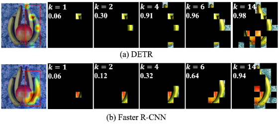
We present an example of analyzing object detectors using explanations generated by VX-CODE. Here, we analyze the differences in behavior between transformer-based and CNN-based architectures. Several studies have explored the differences in characteristics between transformers and CNNs, suggesting that transformers utilize more global information and exhibit more compositionality compared to CNNs [34, 51, 20]. In this experiment, to analyze such differences in object detectors, we use VX-CODE with patch insertion to identify important regions for the same detection results detected by DETR and Faster R-CNN.

Figure O shows the identified patches and generated heat maps for detections of a banana produced by DETR and Faster R-CNN. For DETR, patches in multiple parts are identified in the early steps, and the reward value defined in Eq. 3 reaches $0.91$ after four patches are identified. In contrast, for Faster R-CNN, patches in specific regions are preferentially identified, and the reward value reaches $0.94$ after 14 patches are identified. These results indicate that DETR, a transformer-based architecture, recognizes instances in a more compositional manner and with less information compared to the CNN-based architecture Faster R-CNN.

As demonstrated in this experiment, the explanations obtained from VX-CODE facilitate the analysis of object detectors. Further investigations into such analyses using the proposed method are left for future work.

Explaining Object Detectors via Collective Contribution of Pixels

Abstract

1 Introduction

2 Related Work

2.1 Visual explanations for object detectors

2.2 Visual explanations for classification

3 Approach

3.1 Preliminaries

3.2 Proposed method

3.2.1 Application of Shapley values and interactions to object detectors

3.2.2 Patch identification in VX-CODE

Problem 1

3.2.3 Strategies for further reducing computational cost

4 Experiments

4.1 Evaluation for faithfulness of identified regions

4.2 Qualitative analysis of visualizations

4.3 Analysis of patch selection and step restriction

4.4 Analysis for bias model

4.5 Analysis for bounding box explanations

5 Conclusion

Acknowledgments

References

Appendix A Visual explanations for classification

Appendix B Detailed of the proposed method

B.1 Details of the algorithm

B.2 Specific example of patch insertion

B.2.1 Case with r=1r=1

B.2.2 Case with r=2r=2

B.3 Patch deletion

Problem 2

B.4 Specific example of patch deletion

B.5 Case with r=1r=1

B.6 Case with r=2r=2

B.7 Heat maps generation from identified patches

B.8 Implementation details

Appendix C Additional experimental results

C.1 Additional quantitative results

C.1.1 Pointing game

C.1.2 Analysis for class explanations

C.2 Additional results for visualizations

C.3 Additional results for patch combination

C.4 Additional results for bias model

C.5 Additional results for bounding box explanations

C.6 Multi-perspective explanations for detection results

C.7 Analysis of object detectors using VX-CODE

B.2.1 Case with $r=1$

B.2.2 Case with $r=2$

B.5 Case with $r=1$

B.6 Case with $r=2$