Explaining the cosmological dark matter coincidence in asymmetric dark QCD
Abstract
To properly solve the coincidence problem () in a model of asymmetric dark matter, one cannot simply relate the number densities of visible and dark matter without also relating their particle masses. Following previous work, we consider a framework where the dark matter is a confined state of a dark QCD gauge group whose confinement scale is dynamically related to the QCD confinement scale by a mechanism utilising infrared fixed points of the two gauge couplings. In this work we present a new, ‘zero-coupling infrared fixed point’ approach, which allows a larger proportion of models in this framework to generically relate the masses of the visible and dark matter particles. Due to the heavy mass scale required for the new field content, we introduce supersymmetry to the theory. We consider how these models may be incorporated in a full theory of asymmetric dark matter, presenting some example leptogenesis-like models. We also discuss the phenomenology of these models; in particular, there are gravitational wave signals which, while weak, may be measurable at future mHz and Hz detectors.
I Introduction
The nature of dark matter (DM) remains unknown. While its existence has been firmly established by a range of astrophysical observations, these depend only on its gravitational interactions, and – as the conventional wisdom asserts – provide no indication as to its non-gravitational interactions other than their weakness. However, one clue to its identity that may exist in the present cosmological data is the similarity between the present-day mass fractions of visible matter (VM) and dark matter [1],
| (1) |
which is suggestive of a deep connection between the origins of VM and DM. We refer to this fact as the cosmological coincidence; indeed, this ratio arises coincidentally for most canonical dark matter candidates, such as the WIMP or axion, where the dynamics that generate the cosmological abundances of visible and dark matter are entirely unrelated to each other.
The predominant paradigm that attempts to motivate this relationship is asymmetric dark matter (ADM) [2, 3], where the DM and VM abundances both result from a particle–anti-particle asymmetry generated by some baryogenesis-like mechanism. In ADM models, it is ensured that the number densities are similar, , either dynamically or through the imposition of a symmetry. However, such a mechanism alone does not resolve the cosmological coincidence; to explain the relationship of Eqn. 1 also requires an explanation for 111There have also been attempts to resolve the coincidence problem that directly relate the cosmological mass densities of VM and DM without requiring the number densities and particle masses to both be of a similar order. These arise from anthropic arguments [4, 5, 6] or from some novel dynamics [7, 8]..
The main approach to this problem is to introduce a dark QCD-like gauge group and some mechanism that relates the confinement scale to the QCD confinement scale ; the DM candidate in these models is thus a dark baryon whose mass is similar to the proton mass [9, 10, 11, 12, 13, 14, 15, 16, 17, 18, 19, 20, 21, 22, 23, 24, 25, 26, 27, 28, 29, 30, 31, 32, 33, 34, 35, 36, 37, 38, 39]. The related confinement scales in these models usually derive from a symmetry between the visible and dark QCD gauge groups, often in the context of mirror matter222In mirror matter models, the dark sector consists of a copy of the SM related to the SM by a ‘mirror’ symmetry. Such a structure is primarily considered a priori, or to reintroduce a fundamental parity symmetry [12, 13, 14, 15, 16, 17, 18, 19, 20, 21, 22, 23, 24, 25, 26, 27, 28, 29, 30], but it can also be used to address the little hierarchy problem in the context of Twin Higgs models [31, 32, 33, 34, 35, 36, 37, 38]., or from some unification at high energies [22, 23, 30, 39]. However, avoiding the imposition of a high-energy symmetry, there is a dynamical approach, introduced by Bai and Schwaller [9], that takes advantage of the possible existence of infrared fixed points (IRFPs) in QCD-like theories [9, 10, 11].
In the framework of Ref. [9], new field content is introduced, charged under one or both of visible and dark QCD. This leads to the coupled renormalisation group (RG) evolution of the coupling constants of each gauge group towards a fixed point in the IR, thereby relating the coupling values, and thus the confinement scales, at low energies. One of the appeals of this approach is its insensitivity to the initial coupling strengths of the two gauge groups in the UV, and it is assumed in Ref. [9] that the results in the IR are completely independent of the initial conditions at high energies. However, in our first paper [11] we showed that this is not the case. After accounting for the dependence of the results on the initial UV gauge couplings, we reassessed the ability of models in this framework to naturally relate and . Considering a simplified version of the framework with and only new field content in fundamental representations of visible and dark QCD, we found a set of ‘viable’ models where one would reasonably expect confinement scales on a similar order of magnitude.
However, our results were not entirely satisfactory. Firstly, the viable models comprised a very small fraction of the models in the framework, and to avoid stringent collider constraints on the new coloured fields, some of the new fields required very high multiplicities. Together, these issues made these models unwieldy and difficult to build upon further. This is a problem, as these models only relate the particle masses of VM and DM; to serve as a complete explanation of the cosmological coincidence problem, we must embed these models within an extended ADM theory.
In this work, our aim is to find models that may be more amenable to further study. We relax the restrictions on the number of dark colours and the representations of the new field content, and consider the ADM mechanisms that could be incorporated in these models. In the pursuit of a framework that more generically produces viable models, we are led to investigate models where both couplings are zero at the IRFP; this represents a new framework, beyond that explored by Bai and Schwaller. We refer to this as the zero-coupling fixed point (ZCFP) approach, distinguishing it from the finite-coupling fixed point (FCFP) approach which we have previously explored. We find that the ZCFP approach can alleviate some of the issues associated with the FCFP approach, notably that (i) viable models can be found more generically, and only require a few additional fields to be introduced, and (ii) the mass scale of new physics is generally greater than a TeV, which prevents the phenomenological tension that was difficult to avoid in the FCFP approach.
However, this second point introduces its own difficulties, as the required mass scale for new physics is generically very high, which introduces a naturalness issue of its own in the running of the Higgs mass parameter. We first look for models where the mass of the new field content is low enough to avoid these issues – that is, TeV-scale – and have some success. However, while these models do exist, they are rare, and so do not improve on the first issue associated with the FCFP approach mentioned above. To consider models with very heavy new field content we then introduce supersymmetry to the framework. Here, we find some quite promising results; in particular, when we find a fairly generic set of viable models.
The paper is organised as follows: in Section II we describe the framework, before evaluating the results of our previous work, and their shortcomings, in Section III. In Section IV we introduce and discuss the zero-coupling fixed point approach, and then search for and identify viable ZCFP models in Section V. Following this, in Section VI we consider how to provide these viable models with an ADM mechanism, focusing on leptogenesis-like mechanisms similar to Ref. [9] in both SUSY and non-SUSY cases. We finish by briefly highlighting some of the phenomenology of this framework, including possible direct-detection and gravitational wave signals, in Section VII, before concluding in Section VIII.
II The framework
The basic ingredients of the framework are a new dark confining gauge group which we refer to as ‘dark QCD’, and a selection of field content charged under one or both of visible and dark QCD. The field content consists of Dirac fermions and complex scalars. For simplicity, we take all the new fields to share a (heavy) mass , bar a number of Dirac fermions () charged only under the fundamental representation of dark QCD. We take these latter fields to be ‘light’ in the sense that their mass is lower than the dark confinement scale . We refer to these fields as ‘dark quarks’ and they confine into a dark baryon with a mass on the scale of , which serves as the dark matter candidate.
We denote a ‘model’ within this framework by its selection of field content. The purpose of these models is to naturally obtain similar confinement scales for visible and dark QCD; the dark baryon then has a mass that is on a similar order of magnitude to the proton mass. We denote a model that achieves this goal a ‘viable’ model.
In this framework, the similarity of the confinement scales results from a dynamical mechanism that relates the coupling constants of each gauge group at low energies. The key equations are the -functions that determine the RG evolution of the couplings. In our previous work [11], we specialised to and only considered field content in the fundamental representations of visible and dark QCD; in this work, we relax those assumptions. Here we give the -functions for the strong coupling constant and dark coupling constant , and respectively, which are coupled at two-loop level due to the presence of fields charged under both gauge groups. These are presented for an arbitrary selection of field content of arbitrary representation, where is the multiplicity of a Dirac fermion () or complex scalar () in the representation of 333In this work, some of the representations we consider are real, like the when . Fields in such representations could be included as Majorana fermions or real scalars. We do not account for models with such fields in this framework. As we shall see in Section VI, in realistic models accommodating a baryogenesis mechanism the fields we introduce generally have a non-zero hypercharge, and so are not in real representations of the full gauge theory., and is the set of all multiplicities for the fermions or scalars included in the model. The two-loop -function for is then given by [40]
| (2) |
and is found by exchanging and and interchanging the indices . Here, and are the quadratic Casimirs of the adjoint representations, and for a given representation , is the dimension of the representation, is its quadratic Casimir, and is its Dynkin index.
In this work, we also consider supersymmetric versions of the framework; this avoids the naturalness issue that arises in models with a very high mass scale . In this case, the new field content consists of chiral supermultiplets, each containing a chiral fermion and a complex scalar. We specify the multiplicity of a chiral supermultiplet in the representation of by , and the set of all multiplicities of the supermultiplets included in the model by . The two-loop -function for is then given by [40]
| (3) |
and is found by exchanging and , and interchanging the indices , as before.
The mechanism by which these models naturally relate the confinement scales was first introduced by Bai and Schwaller [9]. The general idea is that, for certain models, the selection of field content is such that the coupled -functions exhibit an infrared fixed point (IRFP). The couplings, which may be be initially unrelated in the UV, evolve towards the IRFP, and are thus dynamically related to each other in the IR, despite the absence of a discrete symmetry that interchanges the visible and dark QCD gauge sectors. After the new field content decouples below its mass scale , the IRFP is broken and the gauge couplings run until they each become non-perturbative and their associated gauge interactions become confining; the relationship between the couplings at the IRFP then leads to a relationship between the confinement scales.
In their initial work, Bai and Schwaller assumed that the couplings reach their IRFP values by the decoupling scale, which was generally TeV-scale. However, in Ref. [11] we showed this to be untrue; the couplings only approach their fixed point values without reaching them. The dark confinement scale predicted for a given model then depends upon the initial conditions for the couplings in the UV. Accounting for this dependence, we then considered a viable model to be one that obtains similar confinement scales for the two sectors for a decent proportion of the parameter space. In this context, we defined a heuristic to judge the viability of a given model which we called the ‘viability fraction’ : it is defined as the proportion of the UV coupling parameter space for which is between 0.2 and 5 GeV.
The viability fraction is the main tool we use to assess the ability of given model to serve as an explanation of the cosmological coincidence problem. The idea is that in a model with a decently large value of , there is a reasonable chance that the confinement scales will be on the same order of magnitude for a random selection of initial values for the coupling constants in the UV. Of course, the distribution from which these values are selected is unknown. The viability fraction we define is merely a simple implementation of this concept, but it is by no means the only one. We also note that these models do not solve the cosmological coincidence problem alone; rather, they provide a template that must be embedded within a full ADM model. In the full theory, a baryogenesis mechanism is required that generates related number densities for visible and dark matter. We return to this question in Section VI.
III The finite-coupling infrared fixed point approach
In this section we provide an evaluation of the key conclusions of our previous work [11]. Our goal there was to identify models within the framework that could viably explain the coincidence problem. Here we identify common features of these viable models, and in particular focus on their shortcomings, namely:
-
1.
These viable models comprise a very small proportion of the total space of models.
-
2.
Most viable models require a sub-TeV mass scale for the new physics, i.e. new sub-TeV coloured states that would be copiously produced at colliders. While we do find viable models with TeV, they generally require large multiplicities for the new fields introduced.
Both of these issues make it difficult for these models to be incorporated within a full ADM model. The purpose of this section is to motivate the approach we take in the following section, which seeks to alleviate these issues.
III.1 Obtaining a finite-coupling fixed point
A fixed point of the coupled RG evolution of the gauge couplings of visible and dark QCD, denoted , is given by
| (4) |
Rewriting Eqn. II as
| (5) |
and with given by exchanging and and interchanging the indices , there are four solutions to Eqn. 4:
| (6) | ||||
| (7) | ||||
| (8) | ||||
| (9) |
Note that these are not necessarily infrared fixed points; they may be UV fixed points, or they may be saddle points of the coupled evolution of the gauge couplings. Indeed, these nominal solutions are not necessarily physical, let alone perturbative.
In our previous work, we considered models in which the last of these solutions – Eqn. 9 – is an infrared fixed point, with both and taking perturbative values444In this work, we consider gauge couplings to be perturbative. This ensures the pertubative validity of our two-loop -function calculations: see Sec. V A in our previous work [11].. This is not the only case one could consider, and so we refer to this case specifically as the ‘finite-coupling fixed point’ approach. This contrasts it with the case we consider in the next section, the ‘zero-coupling fixed point’ approach, where the first of these solutions – Eqn. 6 – is an infrared fixed point.
In Eqn. 9 we immediately see one of the shortcomings that this approach faces; that is, the values of and have a highly non-trivial dependence on the various -function coefficients. Firstly, this prevents any simple links being drawn between the field content of a given model and the value of the couplings at the fixed point, especially since a given field contributes to multiple -function coefficients. Secondly, as stated already, for a generic model these values may not be perturbative, or even physical. To obtain a model that has a perturbative FCFP requires a delicate interplay between the -function coefficients, and we find that this occurs in only a small fraction of models. For example, in our previous work we initially analysed a set of 12,288 models; of these models, 1354 (10%) have an infrared fixed point, and only 155 (1%) of the models have a perturbative fixed point.
The last observation we make here is that for the FCFP of Eqn. 9 to be an infrared fixed point, and must both be negative. The argument is as follows: if the theory contains an infrared FCFP, then initially small couplings must increase towards the IRFP with decreasing energy scale (that is, the zero-coupling fixed point of Eqn. 6 must be a UV fixed point). So, for these small couplings, the -functions must be negative; also, for small couplings the -functions are dominated by the one-loop terms. Thus, the one-loop coefficients and must be negative.
III.2 Large viability fractions
We search for models with the largest possible value for the viability fraction. In our previous work, the largest value we found for was around 0.4, and we considered models with to be viable. These comprised a smaller fraction again of the total models. For example, in the set of 12,288 models mentioned previously, of the 155 models with perturbative infrared FCFPs, only 19 had , comprising 0.1% of the total models.
This restriction is due to the fact that the models with the largest viability fractions all have ‘small’ IRFPs with . The reason for this is in two parts. Firstly, at the decoupling scale of the new physics, we need in order to be able to match the strong coupling to its measured value at the mass, and thus to calculate . So, for this to be achieved for a wide range of initial coupling values in the UV, must be evolving towards a fixed point value . Secondly, to have for a large area of the UV coupling parameter space, we need and to be similar in size at the decoupling scale. This indicates that the couplings should be evolving towards fixed points with similar values. Since must be small, must also be small.
We note that this second point assumes that similar gauge couplings at the decoupling scale imply similar confinement scales in the two sectors. This is only true if the gauge coupling evolution is similar in the two sectors after decoupling. If , or if the number of light dark quarks differs substantially from the number of light SM quarks, then this is not necessarily true. Indeed, we find in general that the value of depends strongly on the number of light dark quarks; this will be discussed further in Section V.
We also note that the intuitive concept of the success of a viable model now differs from the original idea of Bai and Schwaller. The relationship between the couplings in the infrared results from their evolution towards some fixed point whose couplings take small values; that is, they are ‘focused’ toward a point near the origin of the coupling plane, and thus brought close to each other in value. This motivates us to consider the zero-coupling fixed point approach that we introduce in the next section, where the origin itself, , serves as the infrared fixed point that draws the couplings together from their values in the UV.
III.3 The mass scale of new physics
An issue that arises generically for these viable models is that in much of the parameter space, the required mass scale of new physics is below a TeV. These new coloured particles with GeV masses would be copiously produced at colliders, leading to the exclusion of these models. In our previous work, we thus searched for models in which is TeV-scale or higher.
The general idea is that to obtain a high mass scale, the running of the gauge couplings in the full theory must be ‘fast’, so that evolving from the UV matches to the required coupling to generate at a sufficiently high scale. Strong running requires large values for the -function coefficients. In the FCFP approach, the one-loop -function coefficients and must be negative, but there is no restriction on the sign of the two-loop terms. So, the strongest running occurs when and are negative and close to zero. This, however, requires a fine cancellation between the gauge and matter contributions to these coefficients, and so again only occurs for select sets of field content, further reducing the proportion of total models that are viable and phenomenologically allowed.
In our first paper, we achieved strong running by considering models with high multiplicities for the jointly-charged scalars, while finding that successful models also had large multiplicities for the other heavy new scalars. Each additional scalar contributes to all -function coefficients, and so strengthens the running more than scalars charged under only one gauge group.
We note that this means that we are considering models in which the one-loop coefficients are much smaller in magnitude than the two-loop coefficients, thanks to the precise cancellation between the gauge and matter contributions to the one-loop coefficient. This could lead to questions about the perturbative validity of this analysis. Our answer is to consider the magnitude of each term that contributes to a given coefficient, not their sum (as this ignores the artificial smallness that occurs due to cancellations between terms), and to ensure that individual two-loop terms are smaller in magnitude than individual one-loop terms.
The issue now is that not only do these successful models comprise a very small proportion of the parameter space, they also require specific and unwieldly selections of field content, with ten or more joint scalars, and up to nineteen dark scalars555See Fig. 10 of Ref. [11]..
To summarise the conclusions of our previous work regarding the FCFP approach:
-
•
For a model to have a perturbative FCFP, there must be a precise cancellation between combinations of different -function coefficients. In addition, to obtain a decently large value for , the couplings at the fixed point must be small. This means that only a very small proportion of models () even have such a fixed point.
-
•
To then have TeV in most of the UV-coupling parameter space, we need the couplings to run strongly in the full theory while keeping the one-loop -function coefficients negative to ensure the existence of an infrared FCFP. This requires large multiplicities for certain fields, e.g. jointly-charged scalars.
IV The zero-coupling infrared fixed point approach
In this section we consider models in which the zero-coupling fixed point of Eqn. 6, , is an infrared fixed point. This is intended to address the issues with the FCFP approach identified in the previous section, with the benefits being as follows:
-
•
A large proportion of models have an infrared ZCFP, and so viable models can be found more generically within this framework.
-
•
Models including fields in higher-dimensional representations of achieve infrared ZCFPs with small field multiplicities.
-
•
In these models, the running of the gauge couplings is generically strong in the full theory, such that the mass scale of new physics is well above the TeV scale.
In the previous section it was noted that FCFPs with small coupling values produced the largest viability fractions, with an intuitive explanation being that the initial UV couplings and are ‘focused’ towards the small fixed point, and thus brought close to each other in value at lower energy scales. A zero-coupling infrared fixed point has the same ‘focusing’ effect on the gauge couplings, and so it is reasonable to expect that models with such an IRFP may have decent values of .
However, this approach comes with an inherent issue that we have already mentioned: the inclusion of Dirac fermions and complex scalars with large masses introduces a naturalness issue, as they contribute to the running of the Higgs mass parameter. These contributions become significant for new physics with masses in the 10s–100s of TeV [41], while in Section V we generally consider models with GeV. For such models, we are thus led to incorporate supersymmetry within the framework.
IV.1 Obtaining a zero-coupling infrared fixed point
The zero-coupling point is trivially always a fixed point of the RG evolution. For it to be an infrared fixed point, the -functions must be positive for gauge couplings in the vicinity of the fixed point: that is, for small couplings . In this regime, the one-loop terms dominate, and so the one-loop -function coefficients must be positive:
| (10) |
This is a much less restrictive requirement than the delicate cancellations that we needed to obtain an infrared FCFP. Since matter contributions to the -function coefficients are positive, all a model needs in order to have an infrared ZCFP is a sufficient amount of new field content such that the one-loop terms become positive.
In addition, infrared ZCFPs can be achieved generically with low multiplicities for the new field content, thanks to the presence of fields in higher-dimensional representations of both visible and dark QCD. These fields contribute more strongly to the -function coefficients in Eqn. II, due to their high dimension and larger group theory factors. So, for example, if , a model with 6 quarks, 1 dark quark, and just a single fermion exhibits an infrared ZCFP.
To see which higher-dimensional representations have this effect of obtaining infrared ZCFPs with low multiplicities, we consider models containing the 6 SM quarks, 1 dark quark, and some number of copies of an fermion or scalar. In Table 1 we give the minimum number of copies of this field that must be included for a model to exhibit an infrared ZCFP: that is, for the one-loop -function coefficients and to be positive. Fermions of a given representation require smaller multiplicities than the corresponding scalar, since the fermions make a larger contribution to each -function coefficient; this is due in part to Dirac fermions having more degrees of freedom than complex scalars. We also note that models require more higher-dimensional representations than , which correlates with a larger negative gluonic contribution to the -function coefficients.
| 2 | 3 | 4 | |||||||
| 2 | 3 | 4 | 3 | 6 | 8 | 4 | 6 | 10 | |
| 3 | 6 | 4 | 3 | 6 | 2 | 2 | 7 | 4 | 2 |
| 6 | 2 | 1 | 1 | 3 | 1 | 1 | 4 | 2 | 1 |
| 8 | 2 | 1 | 1 | 2 | 1 | 1 | 3 | 2 | 1 |
| (a) fermion | |||||||||
| 2 | 3 | 4 | |||||||
| 2 | 3 | 4 | 3 | 6 | 8 | 4 | 6 | 10 | |
| 3 | 22 | 15 | 11 | 21 | 8 | 6 | 28 | 14 | 5 |
| 6 | 7 | 3 | 3 | 11 | 3 | 2 | 14 | 7 | 3 |
| 8 | 5 | 3 | 2 | 8 | 2 | 2 | 11 | 6 | 2 |
| (b) scalar | |||||||||
IV.2 Asymptotic freedom
One may be perturbed by the fact that positive one-loop -function coefficients seem to imply the loss of asymptotic freedom. Indeed, since the gauge couplings grow with increasing energy scale, they diverge at some Landau pole, which we must ensure does not fall below the Planck scale.
We first note that in this framework, and are only positive above the mass scale of new physics. At energies below this scale, when the new heavy fields have decoupled, the running of is SM-like, and the running of is similar so long as is not too large; so, the theory is asymptotically free at low energies.
The values of the gauge couplings at high energies, and thus the location of the Landau pole, depend upon the mass scale at which the RG evolution changes. In our calculations, we begin by specifying a pair of (perturbative) gauge couplings at the UV scale, , and then solve for by matching to its measured value at . This ensures that we only ever consider mass scales for which each coupling is perturbative from its associated confinement scale all the way up to the Planck scale.
Indeed, the philosophy behind our idea of a model that ‘naturally’ explains the coincidence problem is that we are agnostic to physics above the UV scale. We thus treat and as input parameters, and when defining the viability fraction we consider them to take perturbative values that are randomly, uniformly and independently chosen. This ‘flat prior’ may well be invalid, as the ‘initial’ gauge coupling values in the UV are in fact generated by the unknown high-scale physics. This physics above the Planck scale may also change the RG evolution, avoiding a Landau pole in the theory by either regaining asymptotic freedom, or by the couplings approaching an UV fixed point as in the ‘asymptotic safety’ idea [42, 43, 44]. But, given our ignorance of specific Planck-scale scenarios for generating the coupling constant values, a flat prior is justified.
IV.3 The mass scale of new physics
Models with an infrared ZCFP generally require a high mass scale for the new physics. In these models, the positive -function coefficients in the full theory lead to strong running of the gauge couplings from their initial values in the UV, unless there is a precise cancellation such that the -function coefficients happen to be small. As a result of this ‘fast’ RG evolution, to generate the correct value for at , the new physics must generically decouple at a high scale.
We illustrate this analytically at one-loop level. Ignoring threshold corrections, for a given value of the strong coupling in the UV, , the mass scale for the new physics is found by running up from using the SM RGE, and down from using the RGE of the full theory until they meet. At one-loop level, this is given by
| (11) |
where is the one-loop -function coefficient for QCD with quark flavours, and is the one-loop coefficient for the full theory. Taking the maximum value of gives the minimum value for the mass scale as
| (12) |
While the resultant mass scale can be low, this requires to be small. As will be discussed shortly, cannot be more than 100s of TeV without introducing a severe naturalness issue. To obtain such a mass scale,
| (13) |
For this to occur, the matter contribution to must cancel closely with the gluonic contribution. We encountered a similar restriction in the FCFP approach when searching for models with a sufficiently large value of , and in that case we required specific and unwieldy selections of field content. We find similar behaviour in this case, which we explore in Section V.1.
We identified earlier that we would be interested in models containing fields in higher-dimensional representations, as these models generically obtain an infrared ZCFP with low multiplicities for the new fields. However, it is the inclusion of such representations that strengthens the running to the point that the mass scale is very high. For example, for , models including a fermion have , leading to GeV.
In Table 2 we show the minimum mass scales of new physics for models including a single fermion in the representation . We only show the representations for which a model with the 6 SM quarks, 1 dark quark, and 1 fermion has an infrared ZCFP: that is, the representations in Table 1 with minimum multiplicity 1. We reiterate that these are only the minimum values for , calculated at one-loop; using the two-loop RGEs, working with any UV coupling below , and including any additional field content in these models only increases .
| 2 | 3 | 4 | |||
| 3 | 4 | 6 | 8 | 10 | |
| 6 | |||||
| 8 | |||||
IV.4 Naturalness and a heavy mass scale
We now come to the naturalness issue that arises due to the presence of heavy new physics. As we have seen, the ZCFP approach to this framework generally necessitates such heavy fields.
Dirac fermions and complex scalars contribute to the running of the Higgs mass parameter. If these fields are sufficiently heavy, then these contributions are sizeable, making its low-energy value very sensitive to physics at a high scale. This is true even for coloured fermions, which only contribute to the Higgs mass parameter at three-loop level.
To assess the scale of this issue, we adopt the approach of Ref. [41], where a model is unnatural if, given a flat prior for the Higgs mass parameter in the UV, it is very unlikely for it to obtain its measured value at . This is similar in spirit to our perspective on naturalness, but is implemented quantitatively using a Bayesian sensitivity measure that can be roughly interpreted as a level of fine-tuning.
In Ref. [41], limits are placed on the masses of new gauge multiplets added to the SM. These limits are calculated for threshold values of the sensitivity measure; we look at the results corresponding to a 10% fine-tuning, where for colour-triplet, electroweak-singlet Dirac fermions, the limits are in the 10—100 TeV mass range, and for colour-triplet, electroweak-singlet complex scalars, the limits are in the 1—10 TeV mass range.
We note that these limits on may be optimistic for the models we consider. Firstly, they only apply to colour triplets; any field in a higher-dimensional representation of will be subject to a stronger constraint. Secondly, these limits are calculated for models that only have a single additional gauge multiplet. In models where multiple new fermions and scalars are introduced, must be smaller again to avoid excessive fine-tuning. For these reasons it is possible that even for models with TeV the naturalness issue could remain problematic. This suggests that it could even be impossible to find models in this framework that avoid a naturalness problem, an observation which also applies to the FCFP approach.
IV.5 Supersymmetry
To consider models in which the mass scale is much greater than 100s of TeV, we introduce supersymmetry, which prevents the new heavy fields from contributing to the running of the Higgs mass parameter. We always take the scale of supersymmetry breaking to be TeV. Below the running is as before, with the running of due to light dark quarks. Between and the gauge couplings run separately; the RG evolution of is MSSM-like, and the RG evolution of is due to light dark quarks and light dark squarks.
The heavy field content in this case consists of chiral supermultiplets. In the non-SUSY case, we introduce Dirac fermions and complex scalars to ensure anomaly cancellation and write down renormalisable mass terms. For the same reasons, in the SUSY case when we say we introduce a ‘field’ in the representation of visible and dark QCD, we are adding two chiral supermultiplets and with superpotential mass term .
Introducing SUSY slightly alters the conclusions we made previously in this section about the existence of a zero-coupling IRFP and the size of the mass scale in these models.
In Table 3, we replicate Table 1 in the supersymmetric case. We find that with SUSY, even fewer copies of each new field are required for a model to exhibit a zero-coupling infrared fixed point. This is expected, as each new field we introduce is a pair of chiral supermultiplets containing the same field content as a Dirac fermion and two complex scalars.
| 2 | 3 | 4 | |||||||
| 2 | 3 | 4 | 3 | 6 | 8 | 4 | 6 | 10 | |
| 3 | 2 | 2 | 1 | 3 | 1 | 1 | 4 | 2 | 1 |
| 6 | 1 | 1 | 1 | 2 | 1 | 1 | 2 | 1 | 1 |
| 8 | 1 | 1 | 1 | 1 | 1 | 1 | 2 | 1 | 1 |
We also find that the required mass scale is larger when SUSY is included. For a given , at one-loop level and ignoring threshold corrections, is found by
| (14) |
where the the one-loop -function coefficient . Since the MSSM running is weaker than the SM running, to match the measured strong coupling , the heavy fields must decouple at a higher scale. With TeV and again taking , the minimum value for the mass scale in the SUSY case is
| (15) |
In Table 4 we replicate Table 2 for the SUSY case, showing the minimum mass scales of new physics for models including a single field in the representation . As before, we only show the values of for representations where a model with the 6 SM (s)quarks, 1 dark (s)quark, and 1 field has an infrared ZCFP. Since this occurs for lower-dimensional representations in the SUSY case, more values of are shown than in Table 2. There are also two representations marked with crosses; these models do happen to have a small value of , and so in fact have . This is not possible, and indicates that one cannot solve for in such a model for .
As a comparison to the point singled out in the non-SUSY case, for , models including a field have , leading to GeV.
Finally, we note that although these heavy superfields do not introduce a naturalness issue, we still include their mass scales as they are relevant for some of the discussion in Section VI.
| 2 | 3 | 4 | |||||||
|---|---|---|---|---|---|---|---|---|---|
| 2 | 3 | 4 | 3 | 6 | 8 | 4 | 6 | 10 | |
| 3 | - | - | - | - | - | ||||
| 6 | - | - | |||||||
| 8 | - | ||||||||
V Finding viable models
In this section we identify models within the zero-coupling fixed point approach that can viably explain the cosmological coincidence problem; that is, models with a sufficiently large value of .
We first consider models without supersymmetry, where we must ensure that the mass scale of new physics is in the 1—100 TeV range to avoid introducing a naturalness issue. We find some successful models, but also illustrate the delicate cancellations required in obtaining this low mass scale.
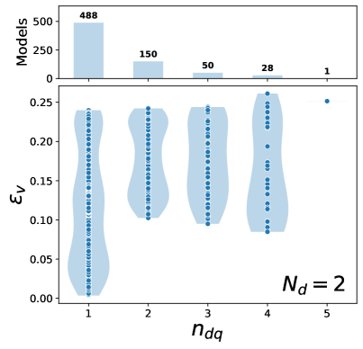
We then look at models incorporating supersymmetry, where a high mass scale is allowed. We find that the viability of a given model depends strongly on the number of light dark quarks, and analyse sets of models for , 3, and 4. We find the most promising results for where most models (65%) have a decently large viability fraction (). For , we find that a decent proportion of models ( 40%) can obtain a decently large viability fraction (), and for we find that less than 1% of models achieve .
V.1 Viable models with a low mass scale
To find models with a low mass scale of new physics , we first must specify the upper limit on such that we avoid a naturalness issue from the contribution of these new fields to the running of the Higgs mass parameter. As mentioned in the previous section, we are guided by the results of Ref. [41] which provides limits on the mass of new Dirac fermion and complex scalar gauge multiplets. Conservatively, to introduce less than 10% fine-tuning requires:
-
•
TeV for colour-triplet, electroweak-singlet Dirac fermions.
-
•
TeV for colour-triplet, electroweak-singlet complex scalars.
We use these limits as rough criteria for determining whether a model avoids a naturalness problem. For models containing only new fermions we look at the viable proportion of parameter space for which TeV: we call this parameter . For models also containing new scalars we look at the viable proportion of UV coupling parameter space for which TeV: we call this parameter .
So, what conditions do we need to place on a model to have TeV in a sizeable proportion of the UV coupling parameter space?
In the previous section, to one-loop level we found that a one-loop -function coefficient results in a minimum value of between 1 and 100 TeV. This changes when we include the two-loop RG evolution. At two-loop level the running is stronger, and so to obtain the same value of requires a smaller value for . The value of now also depends on , and so for a given model the minimum mass scale occurs for . We now find that
| (16) | |||
| (17) |
V.1.1 Models including scalars
Let us first consider models including new complex scalars, where we are interested in the region of viable UV coupling parameter space with TeV. Clearly is a necessary requirement for such a region to exist; however, it does not ensure that this region will be large. Indeed, we find that a decent value for can only be obtained for the smallest possible value of .
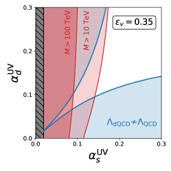
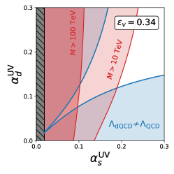
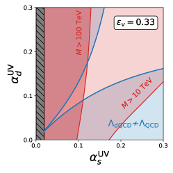
We show this by considering three example models with different values of . We first note that the smallest contribution to the one-loop -function coefficient comes from the scalar, and is equal to ; all other fields contribute some multiple of this amount. So, there are are only three possible values of . In Table 5 we give the field content of the three example models, along with their value of and the minimum mass scale of new physics .
| fermions | scalars | |||||
|---|---|---|---|---|---|---|
| 4 | 1.1 | 0.35 | 0.27 | |||
| 5 | 2.2 | 0.34 | 0.15 | |||
| 6 | 4.2 | 0.33 | 0 |
In Table 5 we also give the value of and for each model. Only the model with the smallest obtains a decent value for . In Fig. 1 we show the relevant and contours in parameter space for these models; in these plots, corresponds to the region between the blue curves and corresponds to the unshaded region.
To obtain such a small value for requires a specific cancellation of the contributions from the gauge and matter content. We would like to achieve this cancellation with low multiplicities for the new fields. To quantify the notion of how rarely these cancellations occur, we consider a simple set of models with at most three of each new field. Since the value of only depends on fields charged under QCD, in these models we only specify the multiplicity of such fields.
Including at most triplet fields, there are 256 total models, of which 5 (2%) have . Including up to sextets, there are now 16 million models, of which only 242 (0.001%) have .
In these models we have not specified the dark field content – that is, fields charged only under . Changing the dark field content changes and ; so, to find viable models with a sufficiently low value of we add dark fields until is decently large. For a given selection of field content charged under QCD, there may be multiple selections of dark field content for which this occurs. In Table 6, we give one such example for each of the 5 models with only new triplet fields, where we have added in a number of light and heavy dark quarks.
When adding dark field content to the 242 models including sextets, we find that most of them are not able to obtain a decent value for . This occurs for two reasons. Firstly, despite these models having the smallest possible value for the one-loop -function coefficient , if the two-loop coefficients are too large, then TeV in only a small region of the UV coupling parameter space. Secondly, if most of the field content is in a higher-dimensional representation of dark QCD than visible QCD, then is larger than even before the addition of any dark field content. The result of this is that is very small, as the stronger running of than in the UV means that similar confinement scales will only be obtained when . This issue only worsens with the inclusion of more dark field content, making even smaller.
Due to these additional difficulties, we find that only 16 of the 242 models with sextets obtain a decent value for . We show the field content of these models in Appendix A. So, while we find that there do exist models with a low enough value of to avoid a naturalness issue, we are in a similar situation to the FCFP approach: these models make up only a very small proportion of the total models, and require several stringent conditions to be satisfied. However, unlike the FCFP approach, these models do not require very large multiplicities for any of the new fields; this makes it more feasible to use these models for further model-building within a full theory of asymmetric dark matter.
| fermions | scalars | |||
|---|---|---|---|---|
| 1 | 0.36 | 0.30 | ||
| 4 | 0.36 | 0.30 | ||
| 3 | 0.37 | 0.33 | ||
| 2 | 0.36 | 0.29 | ||
| 5 | 0.35 | 0.28 |
V.1.2 Models including only fermions
For models only including new heavy fermions, we are interested in the region of viable UV coupling parameter space with TeV. This weaker limit on only really applies for fields that are colour-triplets; higher-dimensional representations of QCD will require at least TeV to avoid the naturalness issue.
The weaker limit on means that these models can have a larger one-loop -function coefficient ; this less stringent restriction should lead to a higher proportion of models with a decent value of . However, Dirac fermions of a given representation make larger contributions to the -function coefficients than the corresponding complex scalar, with the smallest contribution of coming from the fermion. This partially offsets the advantage we gain from allowing larger values for the -function coefficients.
To see how rare these viable models are, we again consider a set of models with at most three of each new field, only specifying the field content charged under QCD. Allowing at most triplets under QCD and sextets under dark QCD, there are 64 models, of which 6 (10%) have .
As before, we add dark field content to these models to see if they can obtain a decent value of . Only three of the models can even obtain a non-zero value for ; we show the field content of these models along with and in Table 7. The other three models face one of the issues identified earlier: they contain too many fields in higher-dimensional representations of dark QCD, and so is larger than before any additional dark field content is introduced.
| fermions | |||
|---|---|---|---|
| 4 | 0.36 | 0.35 | |
| 4 | 0.34 | 0.26 | |
| 1 | 0.36 | 0.18 |
So, we do find that models without a naturalness issue are less rare when only including new fermions; however, the weaker limit on in this case may well be overly optimistic, and the total number of viable models is very low.
Overall, obtaining a sufficiently low value for is achievable, and does not require large multiplicities for the new fields. However, we note that these models ‘only just’ obtain an infrared ZCFP, having small positive values for and . We thus lose part of the appeal of the ZCFP approach, where generic selections of new field content obtain infrared ZCFPs without any specific cancellations. In the next subsection, we seek to take advantage of this feature by considering supersymmetric models with high mass scales.
V.2 Supersymmetric models
In models incorporating SUSY, we face no naturalness issue when adding in new fields. The mass scale of new physics can now be as high as the Planck scale, and there are no restrictions on the size of the -function coefficients as there were in the previous section. This allows us to generically obtain infrared ZCFPs with minimal new field content; in particular we can now include fields of higher-dimensional representations which immediately ensure the existence of an infrared ZCFP.
We are interested in the values of that these models can obtain. The hope is that models in this framework will generically be viable; however we find that this is not always the case. This desire is primarily confronted by the fact that the value of strongly depends on the number of light dark quarks, . This is because changing greatly alters the running of following the decoupling of the new field content, which now occurs at a high mass scale.
In this section we consider sets of models with a given heavy field content; for each selection of heavy field content, we choose the number of light dark quarks such that is a maximum. This is done first for , and then for and 4. A summary of the general findings is as follows:
-
•
For , the best value of is 0.35, which is decently large. However, there is a fairly wide spread of maximum values for , and only a small proportion of models have . While this may challenge our desire to generically obtain viable models, 40% of models have , which constitutes a decent proportion of models with a reasonable viability fraction.
-
•
For , the situation improves. The best value of is 0.42, and 65% of models have .
-
•
For , the situation is worse. There are no models with , and less than 1% even have .
-
•
The required number of light dark quarks peaks at for , for , and for . For a given , the maximum possible value of increases with .
V.2.1 The dependence of on
Before looking at the results for representative sets of models, we first discuss the main issue that makes it difficult for these models to generically obtain decent values of ; that is, the strong dependence of on the number of light dark quarks, .
We note that this dependence on occurs in all versions of this framework, including the models with FCFPs that we considered in our previous work; however, it is more sizeable for the models in this section given their large values for . We illustrate this dependence in Fig. 2 where we show the region of viable UV coupling parameter space for simple models with , a single heavy field, and between 5 and 7 light dark quarks.
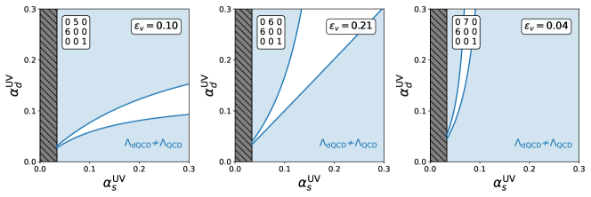
We first note that the viable region seems to ‘rotate’ anti-clockwise as increases. This is generic behaviour, and occurs because, for a given , increasing decreases the value of . The strong dependence of on then comes from the fact that increasing by 1 greatly changes the value of .
To understand this, consider adding a single light dark quark to a model. This additional field only slightly affects the strong running of in the UV, but substantially weakens the running of following the decoupling of the new heavy field content. Also, since depends on the running of , its value stays approximately constant. So, for a given , the weaker running after decoupling leads to reach a non-perturbative value at a lower energy scale. For strong running in the UV and a high value of , a single additional light dark quark will decrease by multiple orders of magnitude.
We show this analytically at one-loop level for , assuming that and the running of in the UV do not change when changes. Then, for a given , the confinement scale for a given , , is found by
| (18) |
where , , and is the one-loop coefficient for the full theory. The factor by which the confinement scale changes when one light dark quark is added is then given by
| (19) |
with a constant given by
| (20) |
We see that the amount by which decreases is larger for larger . Taking typical values of and GeV, for we have
| (21) |
So, for increasing from 5 to 6, we find that decreases by 2 orders of magnitude, and for increasing from 7 to 8, we find that decreases by 3 orders of magnitude.
Finally, we note that, given the general shape of the viable regions in Fig. 2, the models with the largest possible values for should be those where the top-right corner of the parameter space lies within the viable region; that is, GeV for . This helps us understand why only a small proportion of models may have a decent value of . Since at this point changes by multiple orders of magnitude for each additional light dark quark we add, for a given model there will not necessarily be a value of for which the top-right corner of parameter space lies within the viable region.
V.2.2
With we consider a set of selections of heavy field content where we include at most two copies of each new field, and the new fields we introduce are in the , , , , , and representations of . There are 729 such selections of field content, but we are only interested in the models that have an infrared ZCFP. Only 8 of these models lack such a fixed point, since the new field content is mostly in higher-dimensional representations of visible and dark QCD.
For each of these choices of new heavy field content, we add in light dark quarks, choosing the value of such that is a maximum.
We note that to have requires . This is true regardless of the field content in the model, since the maximum possible value of the dark confinement scale, , depends only on . This maximum confinement scale occurs when takes its minimum value; this is the value such that , and defines the edge of the grey hatched region in each UV coupling parameter space plot. We then find when ; for , we have GeV, and so there will be no viable region in the UV coupling parameter space.
In Fig. 3 we plot the maximum values of against for this set of 721 models. The width of the shaded blue region gives the distribution of values for each . We also show the number of models for each value of ; note that the widths of the shaded blue regions are not normalised by these numbers of models. We indeed see that , and in fact no models have a maximum value of for .
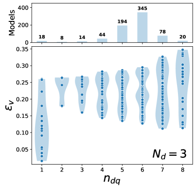
At best, we see that we have . While this is a decent value for , at worst is very close to zero. Even if we discount the cluster of models with and very small viability fractions, can still be as low as 0.12. This challenges our desire for models in this framework to be generically viable; indeed, only 2.5% of these models have , which we have previously used as a threshold for a model to be viable.
However, we do see that 39% of models have . This is a reasonable viability fraction, and so we can state our result as follows: for 2 out of every 5 models in this set of models, when choosing random values for the initial gauge couplings in the UV, there is at least a 1 in 4 chance of having similar confinement scales for visible and dark QCD. We consider this a marked improvement over the coincidence problem as it arises for most canonical dark matter candidates.
In Fig. 3 we also note some interesting trends; in particular, as increases, the maximum possible value of also increases. To explore this, in Fig. 4 we show the viable region of the UV coupling parameter space for the model with the best for each . We see that the viable region changes in shape as we increase , and it seems to be this change in shape that allows for larger to have larger viability fractions.
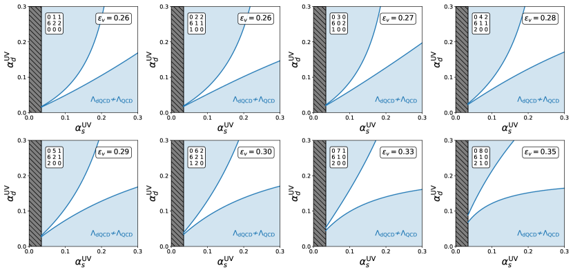
In Fig. 4 the field content of each model is given by the matrix in the top-left corner, using the notation explained in the caption of Fig. 2. We note that as increases, the models change from having more fields above the diagonal of the matrix to having more fields below the diagonal. Above the diagonal, the fields are ‘mostly dark’ – that is, is higher-dimensional than – and below the diagonal they are ‘mostly visible’. So, it seems that for a given model to reach its maximum value of with a high (low) number of light dark quarks, it needs more (less) visible field content than dark field content.
To understand this feature, consider at . As discussed earlier, for to be as large as possible we must have at this point. Now consider a model with . In such a model, since , the running of and will be the same below . So, for visible and dark QCD to have similar confinement scales, the running of and in the full theory must also be similar. The model thus requires similar numbers of mostly-visible and mostly-dark fields; indeed, we see that the model with in Fig. 4 has equal numbers of mostly-visible and mostly-dark fields.
For , the running of is weaker than below . So, to have similar confinement scales for , the running of must also be weaker than in the full theory; for a theory with an infrared ZCFP, this requires that the model has more mostly-visible field content than mostly-dark field content. For , the opposite reasoning applies.
This link between and the selection of field content also explains the distribution we see in the number of models for each , which peaks at . This is the number of light dark quarks for which models with large should have similar numbers of mostly-visible and mostly-dark fields; in the set of models we consider, most models will have such a selection of field content.
We also note that none of the models in Fig. 4 contain a field. This is interesting, and seems to occur because adding a jointly-charged higher-dimensional representation greatly increases the -function coefficients. Larger -function coefficients cause the contours to shrink together slightly, which decreases the maximum possible value of . This can be clearly seen when comparing the model with in Fig. 4 (which has ) to those in Fig. 1. These models, which have low values of , have , and decreases slightly as increases from left to right.
This suggests that, to obtain the largest values of , we in fact do not want to include too many fields in higher-dimensional representations of visible and dark QCD. In our set of models, for the 243 models with a single field, only 2 () have , and there are no models with two fields and . However, this only affects the models with the very largest values of , and the proportion of models with does not change much when fields are included: for , 37% (41%) of models have .
Another effect of adding in fields is to decrease the possible range of such that is a maximum. For , can only be between 3 and 7, and for , can only be between 4 and 7. So, in this sense, including a or similarly higher-dimensional field makes the required number of light dark quarks more predictive.
The last two features of the results in Fig. 3 that we’d like to explain are the cluster of models with and very small viability fractions, and the decrease in the minimum possible value of as increases.
To explain the first of these, we note that the models with small all have many more mostly-dark fields than mostly-visible fields. As we previously showed, such models require a small value of to obtain a decently large . However, for these particular models the running of in the full theory is so much stronger than that even for the running of below is not strong enough to obtain at . The viable region for these models will thus look like the right-most plot of Fig. 2; increasing will only ‘rotate’ the viable region further anti-clockwise, making even smaller.
To understand the second of these features, we again consider the value of the dark confinement scale at ; since reaches its maximum value when GeV at that point, then the minimum value of occurs when is as far from 1 GeV as possible at that point. As we increase for a given set of heavy field content, decreases until for some value of it takes a value below 1 GeV. We now recall that changes by a greater amount when we add a light dark quark to a model that already has a large value of (see Eqn. 20); so, for larger , the dark confinement scale in the top-right corner of parameter space can be further from 1 GeV, leading to a lower minimum value of .
V.2.3
With we consider a set of selections of heavy field content with at most two of each new field, where the new fields we introduce are in the , , , , , and representations of . This is an equivalent set of field content selections to those with , as in both cases we only include fields in the fundamental and lowest-dimensional non-fundamental representations of .
There are 729 such selections of field content; in this case there are only 5 models that lack an infrared ZCFP. As before, for each choice of new heavy field content we find such that is a maximum, and in Fig. 5 we plot the maximum values of against for this set of 724 models.
The results here seem very promising. The best value of is now 0.42, an improvement on . In addition, while can be as low as for some models, the majority of models have a decent viability fraction, with 65% of models having . So, with , it appears that models with an infrared ZCFP are generically viable.
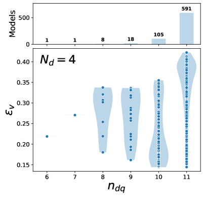
We also note that the number of light dark quarks required for to be a maximum is generally larger, with up to 11; in fact, we see that the majority of models (80%) have . To understand this behaviour, we first note that to have requires . This occurs for the same reasoning we gave earlier; that is, for , GeV. However, for we required ; the fact that larger is allowed when is due to the larger negative gluonic contribution to the coefficients of . Additionally, for we have GeV. This means that can only be very small, despite being non-zero. For this reason, we see that there are no models for which the maximum occurs for .
So, having shown that is necessary for to be a maximum for a given selection of heavy field content, we now explain why the majority of models have exactly this value. We first recall that for , most models have as well as similar numbers of mostly-visible and mostly-dark fields. This is because the running of and is then similar both above and below , such that visible and dark QCD have similar confinement scales for , which ensures that is at a maximum. For , again due to the larger negative gluonic contribution to , models with similar numbers of mostly-visible and mostly-dark fields now have weaker running for than for in the full theory. So, we also need the running of to be weaker than after the new heavy fields decouple, and it is only for that the running of below in these models is weak enough to have at .
So, models with similar numbers of mostly-visible and mostly-dark fields – that is, most models – require . As before, models with more mostly-visible fields require lower to obtain their maximum , as we see in Fig. 6 where we show the viable region of the UV coupling parameter space for the models with the best for each . Again using our earlier reasoning, models with more mostly-dark fields should require larger to obtain their maximum . However, as cannot be greater than 11, the models with more mostly-dark fields instead just have and smaller values of . We observe this behaviour in Fig. 5, where for there is a ‘tail’ of models with lower viability fractions below a cluster around .
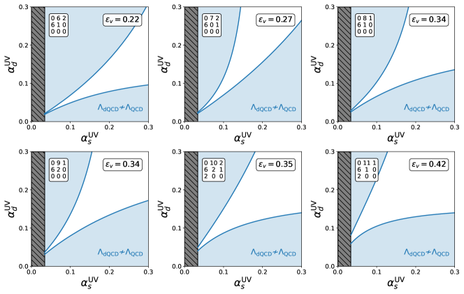
We now wish to understand why there is such a cluster of models at high for , as it is this feature that gives us a large proportion of viable models with . Firstly, the fact that such values of are even possible is due to the fact that these models have a large number of light dark quarks. As we see in Fig. 6, the characteristic shape of the viable regions changes with , and the maximum possible value of increases accordingly. Secondly, to explain the large number of models with , consider a simple model with and a single heavy field. It happens that this model has . We now consider adding in ‘equally visible and dark’ field content to this model: for example, an extra field, or a and a field. This does not substantially change the relative strength of running for and in the full theory, and so the value of does not change much in these models; indeed, the two example models mentioned in the previous sentence both have . So, all such models we construct in this way will have , which leads to the observed cluster of models in Fig. 5.
We note that for the results feature a similar cluster of models. However, in this case, the model with and a single heavy field only has . So for , the cluster of models is at for , as we observe in Fig. 3.
Finally, as before, we see that none of the models in Fig. 6 contain a field, since adding a jointly-charged higher-dimensional representation decreases the maximum possible value of . However, in this case including fields in a model does not reduce the proportion of models with decent . In fact, for it substantially increases the proportion of models, with 75% of those models having .
So, the conclusion of this subsection is that there is a simple set of requirements that generically lead us to viable models: that is, , , and similar numbers of mostly-visible and mostly-dark fields.
V.2.4
Finally in this section, for completeness we briefly mention the case with . With we consider a set of selections of heavy field content with at most two of each new field, where the new fields we introduce are in the , , , , , and representations of . Again, this is an equivalent set of field content selections to before. Of the 729 selections of field content, there are 12 models that lack an infrared ZCFP. Again, for each choice of new heavy field content we find such that is a maximum. In Fig. 7 we plot the maximum values of against for this set of 717 models.
The results in this case are worse than both and . When , the large negative gluonic contributions to mean that must take larger values; here, the gluonic contributions are smaller, and so takes small values, with the majority of models having . The maximum possible value of is smaller for models with smaller values of , and so the best value of is just above 0.25. So, only a very small proportion of models have a decently large viability fraction, with only two models having .
VI Embedding a viable model within a complete asymmetric dark matter model
The viable models we identified in the previous section predict similar masses for visible and dark matter, . To fully explain the cosmological coincidence with one of these models, we now turn to the question of obtaining similar number densities, , by incorporating some asymmetric dark matter mechanism.
Bai and Schwaller [9] considered a simple leptogenesis-like idea that took advantage of the fields charged under both visible and dark QCD. In their model, heavy right-handed neutrinos (RHNs) generate an asymmetry in a new jointly-charged field through their -violating, out-of-equilibrium decays. The subsequent decays of this jointly-charged field distribute the asymmetry to the visible baryons and dark baryons in rougly equal amounts, naturally obtaining related number densities.
We note, however, that the can also couple to visible leptons. In the absence of any new physics that forbids such a coupling, decays thus also introduce an initial visible lepton asymmetry; following sphaleron reprocessing, this asymmetry will be partially converted into a baryon asymmetry, just as in standard thermal leptogenesis [45]. This weakens the relationship between the final visible and dark baryon asymmetries, as it now depends on the couplings of to the visible leptons and the jointly-charged fields; this is similar to the ADM models of Refs. [20, 46]. In this section we first consider this leptogenesis mechanism in a (non-supersymmetric) viable model with a low mass scale , as in Sec. V.1. We find that, assuming similar couplings of to the visible leptons and jointly-charged fields, we still obtain .
We then give a version of this leptogenesis mechanism in a supersymmetric viable model with . We also address the additional difficulties introduced by supersymmetry, where (i) thermal leptogenesis now faces the gravitino problem [47] and (ii) to have the dark baryon be the dark matter candidate, we must ensure that the lightest supersymmetric partner (LSP) is either unstable or only comprises a subdominant component of the dark matter density.
Finally we consider the annihilation of the symmetric component of the dark matter relic density.
VI.1 Leptogenesis in a model with a low mass scale
In this section we consider a version of the leptogenesis model proposed by Bai and Schwaller, looking to incorporate it within one of the viable models identified in Section V.1. In Ref. [9], equal and opposite asymmetries are generated in a fermion and a scalar through their Yukawa interaction with the RHNs . A similar term can produce an asymmetry in any pair of fermion and scalar fields with the same quantum numbers under . The models in Table 7 do not feature such a term, as they only contain new fermions. Of the models in Table 6, all but one feature a fermion and a scalar; the following simple model can be embedded in any of these four models.
Consider a model with a Dirac fermion and a complex scalar . The relevant Lagrangian terms involving the three RHNs are
| (22) |
where we work in a basis where the neutrino masses are real and diagonal. The -violating decays of the produce asymmetries in the new jointly-charged fields, and , in addition to an asymmetry in visible leptons, . In the hierarchical limit , the -asymmetries from each decay are [46]
| (23) | ||||
| (24) |
So, the ratio between the two asymmetry parameters depends upon the relative sizes of the Yukawa couplings, and can be sizeable if there is a hierarchy between the couplings. If the are responsible for the small masses of the SM neutrinos through the seesaw mechanism, then the Yukawa couplings may be hierarchical to generate the observed pattern of masses. Assuming that all other Yukawa couplings are , then the -asymmetry in visible leptons will be much smaller than the jointly-charged fields. If we assume more generically that all Yukawa couplings are of the same order, then , where the larger asymmetry in is due to its higher dimension.
The final asymmetries for , , and are altered by washout effects. For each decay, the washout regime in which it occurs depends upon the decay parameter
| (25) |
where is the total decay rate of , is the branching ratio of its decay into , and is the Hubble expansion rate at . As in Ref. [9], with GeV and Yukawa couplings, both decays are in the strong washout regime where . Then, the final asymmetry can be estimated by [48]
| (26) |
where the number densities are normalised by entropy density as abundance yields and , is the washout decoupling temperature, and is the initial equilibrium abundance of with the number of relativistic degrees of freedom at . In Ref. [9] this asymmetry was found to be large enough to generate the observed visible and dark baryon asymmetries with a mild hierarchy in the RHN masses, , corresponding to .
The ratio between the asymmetries generated by the decay of is
| (27) |
In the case where all Yukawa couplings are of a similar size, this simplifies to for .
We now consider the distribution of these asymmetries into visible and dark baryons through the further decays of and . This occurs just as in Ref. [9]; we introduce a second fermion and dark quarks , with interactions
| (28) |
As in Ref. [9], the interactions of Eqs. 22 and 28 admit an accidental symmetry under which , , , and are odd. This ensures the stability of the dark baryon, which is a confined state of three light dark quarks .
Assuming a slight mass hierarchy , the heavy fields decay via followed by and . This results in baryon, lepton, and dark baryon number densities given by
| (29) | |||
| (30) | |||
| (31) |
Then, following sphaleron reprocessing, the standard leptogenesis relation gives
| (32) |
As discussed earlier, may occur if there is a hierarchy amongst the Yukawa couplings of to the visible leptons, but the are all . If all Yukawa couplings are similar, then following strong washout we have . In both of these cases the ratio of number densities is ,
| (33) |
The number densities would only be unrelated in the unlikely case that there is a strong coupling hierarchy . So, this model manages to relate the number densities of visible and dark matter, despite the multiple decay pathways of the RHNs .
VI.2 Supersymmetric leptogenesis
We now consider implementing this leptogenesis idea in a viable supersymmetric model. We work with , since in Section V.2 we found this allows us to generically obtain viable models. Thermal leptogenesis in supersymmetry has been explored in detail [49, 50, 51, 52], and proceeds in a fairly similar fashion to the standard case. We also note that there are some existing supersymmetric ADM models with leptogenesis-like mechanisms [53, 54], but their implementations differ from ours.
Before giving the details of our model, we mention that within supersymmetry there is a natural mechanism for generating particle asymmetries, the Affleck-Dine mechanism [55, 56, 57, 58], using oscillations along the naturally-occurring flat directions of the superpotential. This is often implemented in ADM scenarios [59, 60, 61], and could be used here to generate an initial asymmetry in a jointly-charged field which subsequently decays into visible and dark baryons. This is a nice idea, but we do not consider it further here.
The new field content required for this model is given in Table 8, where we specify the gauge charges under , along with two other charge assignments that we will discuss shortly. Here, the are singlet chiral superfields with fermionic neutrino and scalar sneutrino components, and we refer to the fermionic and scalar components of the light fields as the dark quarks and dark squarks, respectively. The model is an extension of the -parity–conserving Minimal Supersymmetric Standard Model (MSSM) with superpotential
| (34) | |||
| (35) | |||
| (36) | |||
| (37) |
where we split the additional terms in the superpotential into the mass terms for the new fields, the interaction terms responsible for the initial asymmetry generation through the decay of the , and the interaction terms responsible for the subsequent distribution of these asymmetries into visible and dark baryon asymmetries. For we suppress the generational indices for the light dark (s)quarks , and we work in a basis where the masses of the and the are real and diagonal. Note also that we allow the masses of the new heavy fields to differ from each other slightly, but they all lie close to the required mass scale of new physics, .
The terms in the superpotential (bar the Majorana masses of the ) feature two symmetries, which we treat as extensions of standard baryon and lepton number, naming them and respectively666These charges can also be used to define a discrete ‘matter parity’ symmetry, . This gives all the fields of the MSSM their standard matter parity assignments, and so can be considered as an extension of the standard matter- or -parity. The superpotential of this model respects this symmetry.; their assignments are given in the last two columns of Table 8. The masses of the softly break the extended lepton number, and thus allow for an asymmetry in to be generated through the -violating, out-of-equilibrium decays implied by the superpotential terms of Eqn. 36. If , then these decays of the heavy neutrinos and sneutrinos produce asymmetries in the fermionic and scalar components of the new heavy fields and , where the total asymmetries in each field satisfy ; this is in addition to an asymmetry in visible leptons .
The further decays of the new heavy fields then distribute their asymmetries into visible and dark (s)quarks, where the scalar and fermionic parts of each asymmetry equilibrate through rapid gluino-mediated processes. The visible and dark quarks will eventually confine into the visible baryons and the dark baryons that serve as our dark matter candidate. Before considering the sizes of these asymmetries, let us first discuss the stability of the dark baryon .
The dark baryons are confined states of 4 light dark quarks, with mass a few times . These particles have and , and so are able to decay into SM particles via e.g. . However, this decay is mediated by all the new heavy fields in Table 8, and so is extremely strongly suppressed; this makes the dark baryon very long-lived, and thus sufficiently stable to be the cold dark matter.
In fact, at energies below the mass scale of new physics , all interactions between the dark quarks and SM particles are suppressed by powers of and are thus out of thermal equilibrium. So, at low energies, the particle number of the light dark quarks will be conserved to a very high degree. Let us define the particle number of as , so that the dark baryons have ; at low energies, this ‘dark baryon number’ is approximately conserved.
We now consider the size of the asymmetries generated by the decay of the . In the hierarchical limit for RHN masses, the -asymmetries from each decay in Eqn. 36 are
| (38) | ||||
| (39) |
If all Yukawa couplings are of a similar size, then . In the non-supersymmetric case, we also considered hierarchical Yukawa couplings , as may be needed to generate the observed neutrino masses. In this case, however, the are too heavy to provide sufficiently large neutrino masses with perturbative Yukawa couplings. To do so requires GeV, but to generate asymmetries in the new heavy fields we require , where the mass scale of physics is at least GeV in these models, if not higher (see Table 4)777In general, the neutrino masses can be generated by some alternative mechanism. However, if we do want the to generate the small neutrino masses, then they must have and so cannot decay into the new heavy fields. To generate a dark baryon asymmetry, the would need to have -violating decays to the light dark (s)quarks . This would require some of the to have differing charges..
Another consequence of large is that each decay is in the weak washout regime . In this regime, the final asymmetry depends depends strongly on the initial conditions for the abundance of . Assuming an initial thermal abundance, the final asymmetry can be estimated by [48]
| (40) |
To avoid overproducing the baryon and dark baryon asymmetries, we cannot have all Yukawa couplings be . Achieving the observed baryon-to-entropy ratio of [62] is possible with only somewhat small Yukawa couplings: if some Yukawa couplings are , then with we have , where represents the -violating phases in the complex Yukawa couplings.
However, since is very large, obtaining an initial thermal abundance requires a very high reheating temperature. In the case of vanishing initial -abundance, heavy are produced dynamically by inverse decays, leading to a suppressed final asymmetry given by [48]
| (41) |
In this case, assuming that all Yukawa couplings are of a similar order, the final asymmetry in is given by
| (42) |
and the observed baryon-to-entropy ratio of can be achieved with Yukawa couplings and GeV.
In the weak washout regime, the ratio between the asymmetries generated by the decay of the also depends on its initial conditions, with
| (43) |
If all Yukawa couplings are of a similar size, then . This leads to the initial lepton asymmetry being either somewhat smaller, or much smaller than the initial asymmetry:
| (44) |
We now consider the distribution of these asymmetries into visible and dark baryons. This occurs through the Yukawa and three-scalar interactions implied by the superpotential terms of Eqn. 37. Assuming slight mass hierarchies of and , the asymmetries are distributed to baryons and dark baryons via the decay chains followed by , and followed by . Note that we write each decay in terms of the superfields as a shorthand for the various decays of the fermionic and scalar components of each field.
This gives final baryon, lepton, and dark baryon number densities
| (45) | |||
| (46) | |||
| (47) |
Note that these asymmetries are consistent with the fact that the decays respect and conservation, satisfying .
This initial asymmetry is then subject to sphaleron reprocessing. Since the dark quarks are not in thermal equilibrium with the SM bath at the relevant temperatures, they do not take part in the reprocessing, and the asymmetry is unchanged. In SUSY leptogenesis, the second Higgs doublet needs to be taken into account, resulting in [63]. This gives the final ratio of visible and dark baryon number densities as
| (48) |
Here, if the initial asymmetries in lepton number and the jointly-charged fields are of a similar size, then there is a cancellation that results in . However, if all Yukawa couplings are of a similar size, then , where the relative sizes of these asymmetries depend on the initial abundance as in Eqn. 44. The particular ratio of initial asymmetries does not have a strong effect on the final ratio of visible and dark baryon number densities, which will lie between the following values:
| (49) |
To obtain the observed cosmological coincidence of Eqn. 1 then requires a dark baryon with mass
| (50) |
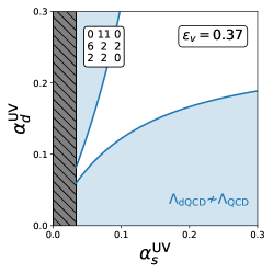
We now consider embedding this set-up within a model with a decent value of . We show such a model in Fig. 8. Its field content contains the two fields and two fields necessary for the above mechanism. In addition, it has two fields and two fields. We can arrange it so that these fields do not take part in the decay chains that redistribute the asymmetries, and so do not alter our earlier calculations: if their gauge quantum numbers are given by and , and they interact through the superpotential terms
| (51) |
then if , any initial thermal population of the new fields will decay into visible and dark baryons through the decays and followed by and , where again we write the decays in terms of superfields as a shorthand. These additional interactions also respect the extended and symmetries, with , , , and .
VI.2.1 Cosmological constraints in supersymmetry
We now discuss some of the additional challenges you face when implementing leptogenesis and asymmetric dark matter mechanisms in a supersymmetric theory: (i) the gravitino problem [47] and (ii) the relic density of the lightest supersymmetric particle (LSP). The latter issue applies to any supersymmetric ADM model, while the former is specific to our proposed leptogenesis-like mechanism; however, we mention them together as they can be solved simultaneously by considering a very light gravitino.
For the first of these problems, gravitinos in general can cause cosmological issues: if they are stable they are at danger of being overproduced, and the decays of unstable gravitinos can lead to the disruption of BBN. Avoiding these scenarios puts various upper bounds on the reheating temperature, with the latter case in particular requiring GeV [47]. The gravitino problem is the conflict between this limit and the necessary RHN mass scale for successful thermal leptogenesis; this is especially problematic in our case, where for the to decay to the new heavy fields we need a large value of at least GeV. However, these limits are derived for a gravitino mass of 100 GeV—10 TeV, as is typical for gravity-mediated supersymmetry breaking. In gauge-mediated supersymmetry breaking scenarios the gravitino mass can be as low as a fraction of an eV, and a sufficiently light gravitino will decay prior to BBN and thus face no limit on the reheating temperature.
The second issue is that, for an ADM model to explain the cosmological coincidence, we need the dark matter density to consist predominantly of the dark baryons whose mass and number density are naturally related to those of the proton. However, in -parity–conserving supersymmetry, the LSP is stable and its relic abundance also contributes to the cosmological dark matter density. We thus need to ensure that any stable LSP is only a subdominant component of the dark matter. A light gravitino with keV decouples while relativistic, and so its relic density is estimated to be [64]
| (52) |
where is the number of relativistic degrees of freedom at its decoupling temperature. Taking [65], the fraction of the DM relic density made up by the gravitino component is
| (53) |
where [1]. Given its small mass, it will behave as a hot dark matter subcomponent, free-streaming and thus facing constraints from cosmic microwave background data and from large-scale structure. The most recent limit on its mass is eV [66], and so an eV-scale gravitino evades these bounds while making only a percent-level contribution to the present-day DM density and avoiding the gravitino problem.
Finally here we mention some alternative solutions to these problems. For the gravitino problem, a low reheating temperature is possible if the initial population of RHNs is produced non-thermally. This can occur naturally in supersymmetry by using oscillations along the flat directions of the superpotential [67]. To deal with the relic abundance of the LSP, we can consider models in which the LSP is unstable. This could occur if -parity is broken, or if a different discrete symmetry such as baryon triality [68] is imposed; however, in this case one would need to be careful to ensure the stability of the dark matter candidate.
VI.3 Annihilating the symmetric component of the dark matter
In ADM models, we need to ensure that only the dark particle–anti-particle asymmetry contributes to the dark matter relic density, by requiring the symmetric component of the DM to annihilate away sufficiently quickly. As noted in Ref. [9], the dark baryons will annihilate efficiently into dark pions, which can then decay into SM fields via interactions mediated by the new jointly-charged fields.
For the non-supersymmetric models where these new fields are TeV-scale, this decay can occur rapidly. In the model of Sec. VI.1, the dark pion decay is mediated by the scalar through the interaction . If the dark pion mass and decay constant are a factor of a few larger than their SM values, such that , then the dark pion can decay into strange quarks with decay width . Taking MeV, this gives a sufficiently short dark pion lifetime of
| (54) |
In the supersymmetric models we consider, however, the new jointly-charged fields are very heavy, and the dark pions are very long-lived. So, we must introduce another annihilation channel for the dark matter. One possibility that takes advantage of SUSY is to consider the nearly-minimal supersymmetric model, which introduces a gauge singlet field in addition to the MSSM particle content. In this theory the scalar component of the singlet is very light, and the dark baryons can decay into it via exchange of the fermionic singlinos [53].
Another general idea is to introduce a new dark gauge symmetry under which the dark baryons are charged, allowing them to annihilate to the dark force carriers. For this to efficiently eliminate the symmetric DM component, the annihilation cross-section must be at least a few times the weak scale [69]. For a gauge symmetry with a fine-structure constant , the cross-section will be sufficiently large for .
If this symmetry is broken, the massive gauge bosons can then decay to the SM. Considering the simplest case of a dark , the massive dark photon can decay to SM charged leptons via kinetic mixing with the photon. For a dark photon with mass MeV, the decay width is , where is the kinetic mixing parameter. At this mass, a kinetic mixing parameter of evades current constraints [70], and also leads to a very short dark pion lifetime,
| (55) |
VII Phenomenology
We now briefly discuss the phenomenology of the models in this framework. In this section we do not consider the non-supersymmetric models with TeV-scale masses for the new fields, as their experimental signatures have already been covered in Ref. [9]. There, the relevant phenomenology arises from the new jointly-charged fields, which mediate DM-nucleon interactions in reach of current direct detection experiments, and can be produced directly at colliders.
In the supersymmetric models we consider, the new fields are very heavy, with a typical mass scale GeV. This suppresses their interactions with SM particles, rendering them undetectable in current experiments. However, these models do still require new physics close to the TeV-scale that makes them accessible, both at colliders and in dark matter direct detection experiments.
Firstly, these models exhibit the standard SUSY collider signatures. We have taken the scale of SUSY-breaking to be TeV to lie above the current strongest constraints on the gluino mass [71], but TeV-scale electroweakinos may be accessible in future experiments such as HL-LHC [72].
Secondly, the efficient annihilation of the symmetric component of the dark matter to SM particles generally requires interactions mediated by new physics with masses at the TeV-scale or lower; these interactions also result in potentially detectable dark matter-nucleon scattering cross-sections.
For example, in Section VI.3 we introduced a broken dark gauge symmetry ; in this case, the kinetic mixing between the photon and the massive dark photon allows the symmetric part of the DM to decay to SM charged leptons, and also mediates spin-independent DM-nucleon scattering. The scattering cross-section is given by , where is the dark baryon comprised of light dark quarks , and is the reduced mass of the DM and nucleon. Taking GeV, and with an allowed kinetic mixing parameter of as before, we have
| (56) |
As before, the fine-structure constant has a lower limit of to ensure efficient annihilation of the symmetric SM component. With , for a 1 GeV dark matter particle the spin-independent scattering cross-section lies close to the neutrino fog [73], and below current experimental limits [74]. With a larger value of , or with a larger dark baryon mass888The required dark matter mass depends on the specific number density ratio resulting from a particular asymmetry generation mechanism. For an value of , we can have up to 15 GeV., the dark matter could be in reach of future direct detection experiments.
All models in this framework also feature a potential stochastic gravitational wave (GW) signal arising from a first-order chiral phase transition in the dark sector [75, 76, 77]. In the SM, it is known from lattice studies that the QCD phase transition is crossover [78, 79], and so does not generate such a signal. This is due to the specific, finite masses of the three light quark flavours, which control the dynamics of the transition. In the limit of massless quarks, a QCD-like group with 3 or more quark flavours will exhibit a first-order phase transition [80, 78]. So, the quark-hadron phase transition of the dark QCD gauge group will be first-order if and the light dark quarks are sufficiently light. Nearly all of the viable models we consider have sufficiently many light dark quarks: for example, looking at the viable supersymmetric models in Section V.2, for only 3% of the models with have , and for all models have .
During a cosmological first-order phase transition, gravitational waves are generated by the collisions of the expanding bubbles of broken phase, and by sound waves and turbulence in the surrounding plasma. For a particular dark sector, determining the strength of the stochastic GW signal requires the calculation of four parameters that characterise the dynamics of the phase transition: the energy released during the transition, ; the terminal bubble wall velocity, ; the bubble nucleation temperature, ; and the duration of the phase transition, . In Ref. [81], calculations of these parameters were reviewed in the context of ADM theories like ours, in which the dark matter is a GeV-scale dark baryon and thus the dark QCD gauge group undergoes a GeV-scale chiral phase transition. There, it was claimed that Hz GW signals could be generated that would be detectable at the proposed detector Ares [82].
However, this conclusion may be optimistic. Given that the dark QCD phase transition in our models has (GeV), the most important parameter in determining the strength and peak frequency of the GW signal is the phase transition duration . The detectable Hz GW spectra identified in Ref. [81] require ; however, studies of the phase transition in QCD-like theories based upon low energy effective models generally find a much shorter phase transition duration . This is common to studies of color confinement in pure Yang-Mills gauge theories from [83, 84] up to [85], and also to dark sectors with 3 or more light dark quarks [86, 87, 88, 89]. The GW spectrum generated by such a phase transition will have a higher peak frequency, typically in the mHz range where space-based interferometers like LISA [90] and BBO [91] are most sensitive. These GW signals generally lie below the sensitivity of the proposed detectors, but there are suggestions that they may be detectable at BBO with (10 GeV). We do note, finally, that these results are derived from effective field theories that attempt to capture complex non-perturbative behaviours. On the advent of more sophisticated, first-principles lattice calculations, it may be that these signals are stronger than expected and have greater prospects of detection.
VIII Conclusions
In this work, we explored a new dark QCD framework in which there is a dynamical mechanism to relate the confinement scales of visible and dark QCD. This provides a dark matter candidate, the dark baryon, whose mass is naturally on a similar order to the proton mass. When combined with an asymmetric dark matter mechanism that relates the number densities of visible and dark matter, this provides an explanation of the coincidental similarity of the cosmological mass densities of visible and dark matter. We followed on from previous work in which new field content is introduced such that the gauge couplings of visible and dark QCD evolve towards a fixed point with small, related values for the two couplings – referred to as the finite-coupling fixed point approach – and instead considered a framework in which the couplings at the infrared fixed point are both zero. In this approach, the initial coupling strengths in the UV both evolve to be very small, before the new field content decouples at a high mass scale. These couplings then evolve independently until the energy scale at which they become non-perturbative and confinement occurs. The visible and dark confinement scales can then be similar for a generic selection of initial values for the couplings in the UV, with the caveat that this depends strongly on the number of light dark quarks.
We analysed models in this framework in order to find viable models that could explain the similarity of the visible and dark confinement scales, looking at dark gauge groups with varying number of colours , and adding in field content in various representations of . We first looked at models where the required mass scale of new physics is (TeV) to avoid naturalness constraints from the running of the Higgs mass parameter. In that case we did find viable models, but they were rare, and required a close cancellation between the matter and gauge contributions to the -function coefficients; this cancellation is similar to that required for the viable models in the FCFP approach. However, in the FCFP approach, the successful models required very large multiplicities for the new field content; here, that was no longer the case.
Secondly, we looked at models in which no such cancellation occurs between the various contributions to the -function coefficients. In these models, the mass scale of new physics is generically very high (only a few orders of magnitude below the UV scale) and so to avoid the naturalness issue for the Higgs mass parameter required us to consider supersymmetric versions of these models. In this case, for different values of we considered generic sets of models with low multiplicities for the new field content we introduce. For each model we chose the number of light dark quarks to maximise the viability fraction , our heuristic that characterises the ability of a given model to explain the similarity of the confinement scales.
The results here were quite promising. In particular, when , we found that 65% of models have , with most of these models requiring 11 light dark quarks. For we found that 40% of models have , with most models requiring 6 dark quarks. For , however, all but a few models were not viable.
These sets of models are intended to be amenable to further development into full models of asymmetric dark matter. In this direction, we showed examples of a leptogenesis-like asymmetry generation mechanism for viable models in both the non-SUSY and SUSY cases. We also highlighted some of the phenomenology of these models. In particular we considered the gravitational wave signals arising from the cosmological chiral phase transition in the dark QCD sector. In this framework this transition is generically first-order and thus features a stochastic GW signal. While these signals usually lie at mHz peak frequencies sensitive to space-based interferometers like LISA and BBO, they are thought to be too weak to be detectable, due to the short duration of the phase transition. However, depending on calculational uncertainties in the GW dynamics, there may be prospects for detection at BBO, or even the proposed Ares detector in the Hz region.
The proposed ADM mechanisms in this paper are not the only possible way to build upon models in this framework. Further studies of the phenomenology and cosmology of complete ADM models incorporating other ADM mechanisms would be welcome.
Acknowledgements
ACR was supported by an Australian Government Research Training Program Scholarship. This research was supported by the Australian Government through the Australian Research Council Centre of Excellence for Dark Matter Particle Physics (CDM, CE200100008).
References
- Aghanim et al. [2020] N. Aghanim et al. (Planck), Planck 2018 results. VI. Cosmological parameters, Astron. Astrophys. 641, A6 (2020), [Erratum: Astron.Astrophys. 652, C4 (2021)], arXiv:1807.06209 [astro-ph.CO] .
- Petraki and Volkas [2013] K. Petraki and R. R. Volkas, Review of asymmetric dark matter, Int. J. Mod. Phys. A 28, 1330028 (2013), arXiv:1305.4939 [hep-ph] .
- Zurek [2014] K. M. Zurek, Asymmetric Dark Matter: Theories, Signatures, and Constraints, Phys. Rept. 537, 91 (2014), arXiv:1308.0338 [hep-ph] .
- Linde [1988] A. D. Linde, Inflation and Axion Cosmology, Phys. Lett. B 201, 437 (1988).
- Wilczek [2004] F. Wilczek, A Model of anthropic reasoning, addressing the dark to ordinary matter coincidence, , 151 (2004), arXiv:hep-ph/0408167 .
- Hellerman and Walcher [2005] S. Hellerman and J. Walcher, Dark matter and the anthropic principle, Phys. Rev. D 72, 123520 (2005), arXiv:hep-th/0508161 .
- Rosa and Silva [2023] J. a. G. Rosa and D. M. C. Silva, Comparable dark matter and baryon abundances with a heavy dark sector, Phys. Lett. B 846, 138178 (2023), arXiv:2211.10359 [hep-ph] .
- Brzeminski and Hook [2023] D. Brzeminski and A. Hook, A Dynamical Explanation of the Dark Matter-Baryon Coincidence, (2023), arXiv:2310.07777 [hep-ph] .
- Bai and Schwaller [2014] Y. Bai and P. Schwaller, Scale of dark QCD, Phys. Rev. D 89, 063522 (2014), arXiv:1306.4676 [hep-ph] .
- Newstead and TerBeek [2014] J. L. Newstead and R. H. TerBeek, Reach of threshold-corrected dark QCD, Phys. Rev. D 90, 074008 (2014), arXiv:1405.7427 [hep-ph] .
- Ritter and Volkas [2023] A. C. Ritter and R. R. Volkas, Exploring the cosmological dark matter coincidence using infrared fixed points, Phys. Rev. D 107, 015029 (2023), arXiv:2210.11011 [hep-ph] .
- Hodges [1993] H. Hodges, Mirror baryons as the dark matter, Phys. Rev. D 47, 456 (1993).
- Berezhiani et al. [1996] Z. G. Berezhiani, A. D. Dolgov, and R. N. Mohapatra, Asymmetric inflationary reheating and the nature of mirror universe, Phys. Lett. B 375, 26 (1996), arXiv:hep-ph/9511221 .
- Mohapatra and Teplitz [2000] R. N. Mohapatra and V. L. Teplitz, Mirror dark matter, in 7th International Symposium on Particles, Strings and Cosmology (2000) pp. 211–221, arXiv:astro-ph/0004046 .
- Berezhiani et al. [2001] Z. Berezhiani, D. Comelli, and F. L. Villante, The Early mirror universe: Inflation, baryogenesis, nucleosynthesis and dark matter, Phys. Lett. B 503, 362 (2001), arXiv:hep-ph/0008105 .
- Ignatiev and Volkas [2003] A. Y. Ignatiev and R. R. Volkas, Mirror dark matter and large scale structure, Phys. Rev. D 68, 023518 (2003), arXiv:hep-ph/0304260 .
- Foot and Volkas [2003] R. Foot and R. R. Volkas, Was ordinary matter synthesized from mirror matter? An Attempt to explain why Omega(Baryon) approximately equal to 0.2 Omega(Dark), Phys. Rev. D 68, 021304 (2003), arXiv:hep-ph/0304261 .
- Foot and Volkas [2004] R. Foot and R. R. Volkas, Explaining Omega(Baryon) approximately 0.2 Omega(Dark) through the synthesis of ordinary matter from mirror matter: A More general analysis, Phys. Rev. D 69, 123510 (2004), arXiv:hep-ph/0402267 .
- Foot [2004] R. Foot, Mirror matter-type dark matter, Int. J. Mod. Phys. D 13, 2161 (2004), arXiv:astro-ph/0407623 .
- An et al. [2010] H. An, S.-L. Chen, R. N. Mohapatra, and Y. Zhang, Leptogenesis as a Common Origin for Matter and Dark Matter, JHEP 03, 124, arXiv:0911.4463 [hep-ph] .
- Cui et al. [2012] J.-W. Cui, H.-J. He, L.-C. Lu, and F.-R. Yin, Spontaneous Mirror Parity Violation, Common Origin of Matter and Dark Matter, and the LHC Signatures, Phys. Rev. D 85, 096003 (2012), arXiv:1110.6893 [hep-ph] .
- Lonsdale and Volkas [2014] S. J. Lonsdale and R. R. Volkas, Grand unified hidden-sector dark matter, Phys. Rev. D 90, 083501 (2014), [Erratum: Phys.Rev.D 91, 129906 (2015)], arXiv:1407.4192 [hep-ph] .
- Lonsdale [2015] S. J. Lonsdale, Unified dark matter with intermediate symmetry breaking scales, Phys. Rev. D 91, 125019 (2015), arXiv:1412.1894 [hep-ph] .
- Lonsdale et al. [2017] S. J. Lonsdale, M. Schroor, and R. R. Volkas, Asymmetric Dark Matter and the hadronic spectra of hidden QCD, Phys. Rev. D 96, 055027 (2017), arXiv:1704.05213 [hep-ph] .
- Lonsdale and Volkas [2018] S. J. Lonsdale and R. R. Volkas, Comprehensive asymmetric dark matter model, Phys. Rev. D 97, 103510 (2018), arXiv:1801.05561 [hep-ph] .
- Ibe et al. [2018] M. Ibe, A. Kamada, S. Kobayashi, and W. Nakano, Composite Asymmetric Dark Matter with a Dark Photon Portal, JHEP 11, 203, arXiv:1805.06876 [hep-ph] .
- Ibe et al. [2019] M. Ibe, A. Kamada, S. Kobayashi, T. Kuwahara, and W. Nakano, Baryon-Dark Matter Coincidence in Mirrored Unification, Phys. Rev. D 100, 075022 (2019), arXiv:1907.03404 [hep-ph] .
- Ritter and Volkas [2021] A. C. Ritter and R. R. Volkas, Implementing asymmetric dark matter and dark electroweak baryogenesis in a mirror two-Higgs-doublet model, Phys. Rev. D 104, 035032 (2021), arXiv:2101.07421 [hep-ph] .
- Ibe et al. [2021] M. Ibe, S. Kobayashi, and K. Watanabe, Chiral composite asymmetric dark matter, JHEP 07, 220, arXiv:2105.07642 [hep-ph] .
- Bodas et al. [2024] A. Bodas, M. A. Buen-Abad, A. Hook, and R. Sundrum, A Closer Look in the Mirror: Reflections on the Matter/Dark Matter Coincidence, (2024), arXiv:2401.12286 [hep-ph] .
- Farina [2015] M. Farina, Asymmetric Twin Dark Matter, JCAP 11, 017, arXiv:1506.03520 [hep-ph] .
- Garcia Garcia et al. [2015] I. Garcia Garcia, R. Lasenby, and J. March-Russell, Twin Higgs Asymmetric Dark Matter, Phys. Rev. Lett. 115, 121801 (2015), arXiv:1505.07410 [hep-ph] .
- Farina et al. [2016] M. Farina, A. Monteux, and C. S. Shin, Twin mechanism for baryon and dark matter asymmetries, Phys. Rev. D 94, 035017 (2016), arXiv:1604.08211 [hep-ph] .
- Terning et al. [2019] J. Terning, C. B. Verhaaren, and K. Zora, Composite Twin Dark Matter, Phys. Rev. D 99, 095020 (2019), arXiv:1902.08211 [hep-ph] .
- Beauchesne [2020] H. Beauchesne, Mirror neutrons as dark matter in the Mirror Twin Two Higgs Doublet Model, JHEP 09, 048, arXiv:2007.00052 [hep-ph] .
- Feng and Yu [2020] W.-Z. Feng and J.-H. Yu, Twin Cogenesis, (2020), arXiv:2005.06471 [hep-ph] .
- Bittar et al. [2023] P. Bittar, G. Burdman, and L. Kiriliuk, Baryogenesis and dark matter in the mirror twin Higgs, JHEP 11, 043, arXiv:2307.04662 [hep-ph] .
- Alonso-Álvarez et al. [2023] G. Alonso-Álvarez, D. Curtin, A. Rasovic, and Z. Yuan, Baryogenesis through Asymmetric Reheating in the Mirror Twin Higgs, (2023), arXiv:2311.06341 [hep-ph] .
- Murgui and Zurek [2022] C. Murgui and K. M. Zurek, Dark unification: A UV-complete theory of asymmetric dark matter, Phys. Rev. D 105, 095002 (2022), arXiv:2112.08374 [hep-ph] .
- Jones [1982] D. R. T. Jones, The Two Loop beta Function for a G(1) x G(2) Gauge Theory, Phys. Rev. D 25, 581 (1982).
- Clarke and Cox [2017] J. D. Clarke and P. Cox, Naturalness made easy: two-loop naturalness bounds on minimal SM extensions, JHEP 02, 129, arXiv:1607.07446 [hep-ph] .
- Weinberg [1976] S. Weinberg, Critical Phenomena for Field Theorists, in 14th International School of Subnuclear Physics: Understanding the Fundamental Constitutents of Matter (1976).
- Weinberg [1980] S. Weinberg, Ultraviolet Divergences in Quantum Theories of Gravitation, in General Relativity: An Einstein Centenary Survey (1980) pp. 790–831.
- Bonanno et al. [2020] A. Bonanno, A. Eichhorn, H. Gies, J. M. Pawlowski, R. Percacci, M. Reuter, F. Saueressig, and G. P. Vacca, Critical reflections on asymptotically safe gravity, Front. in Phys. 8, 269 (2020), arXiv:2004.06810 [gr-qc] .
- Fukugita and Yanagida [1986] M. Fukugita and T. Yanagida, Baryogenesis Without Grand Unification, Phys. Lett. B 174, 45 (1986).
- Falkowski et al. [2011] A. Falkowski, J. T. Ruderman, and T. Volansky, Asymmetric Dark Matter from Leptogenesis, JHEP 05, 106, arXiv:1101.4936 [hep-ph] .
- Kawasaki et al. [2008] M. Kawasaki, K. Kohri, T. Moroi, and A. Yotsuyanagi, Big-Bang Nucleosynthesis and Gravitino, Phys. Rev. D 78, 065011 (2008), arXiv:0804.3745 [hep-ph] .
- Buchmuller et al. [2005a] W. Buchmuller, P. Di Bari, and M. Plumacher, Leptogenesis for pedestrians, Annals Phys. 315, 305 (2005a), arXiv:hep-ph/0401240 .
- Covi et al. [1996] L. Covi, E. Roulet, and F. Vissani, CP violating decays in leptogenesis scenarios, Phys. Lett. B 384, 169 (1996), arXiv:hep-ph/9605319 .
- Giudice et al. [2004] G. F. Giudice, A. Notari, M. Raidal, A. Riotto, and A. Strumia, Towards a complete theory of thermal leptogenesis in the SM and MSSM, Nucl. Phys. B 685, 89 (2004), arXiv:hep-ph/0310123 .
- Buchmuller et al. [2005b] W. Buchmuller, R. D. Peccei, and T. Yanagida, Leptogenesis as the origin of matter, Ann. Rev. Nucl. Part. Sci. 55, 311 (2005b), arXiv:hep-ph/0502169 .
- Fong et al. [2010] C. S. Fong, M. C. Gonzalez-Garcia, E. Nardi, and J. Racker, Supersymmetric Leptogenesis, JCAP 12, 013, arXiv:1009.0003 [hep-ph] .
- Haba and Matsumoto [2011] N. Haba and S. Matsumoto, Baryogenesis from Dark Sector, Prog. Theor. Phys. 125, 1311 (2011), arXiv:1008.2487 [hep-ph] .
- Choi et al. [2013] K.-Y. Choi, E. J. Chun, and C. S. Shin, Dark matter asymmetry in supersymmetric Dirac leptogenesis, Phys. Lett. B 723, 90 (2013), arXiv:1211.5409 [hep-ph] .
- Affleck and Dine [1985] I. Affleck and M. Dine, A New Mechanism for Baryogenesis, Nucl. Phys. B 249, 361 (1985).
- Linde [1985] A. D. Linde, The New Mechanism of Baryogenesis and the Inflationary Universe, Phys. Lett. B 160, 243 (1985).
- Dine et al. [1996] M. Dine, L. Randall, and S. D. Thomas, Baryogenesis from flat directions of the supersymmetric standard model, Nucl. Phys. B 458, 291 (1996), arXiv:hep-ph/9507453 .
- Dine and Kusenko [2003] M. Dine and A. Kusenko, The Origin of the matter - antimatter asymmetry, Rev. Mod. Phys. 76, 1 (2003), arXiv:hep-ph/0303065 .
- Bell et al. [2011] N. F. Bell, K. Petraki, I. M. Shoemaker, and R. R. Volkas, Pangenesis in a Baryon-Symmetric Universe: Dark and Visible Matter via the Affleck-Dine Mechanism, Phys. Rev. D 84, 123505 (2011), arXiv:1105.3730 [hep-ph] .
- Cheung and Zurek [2011] C. Cheung and K. M. Zurek, Affleck-Dine Cogenesis, Phys. Rev. D 84, 035007 (2011), arXiv:1105.4612 [hep-ph] .
- von Harling et al. [2012] B. von Harling, K. Petraki, and R. R. Volkas, Affleck-Dine dynamics and the dark sector of pangenesis, JCAP 05, 021, arXiv:1201.2200 [hep-ph] .
- Fong et al. [2012] C. S. Fong, E. Nardi, and A. Riotto, Leptogenesis in the Universe, Adv. High Energy Phys. 2012, 158303 (2012), arXiv:1301.3062 [hep-ph] .
- Khlebnikov and Shaposhnikov [1996] S. Y. Khlebnikov and M. E. Shaposhnikov, Melting of the Higgs vacuum: Conserved numbers at high temperature, Phys. Lett. B 387, 817 (1996), arXiv:hep-ph/9607386 .
- Viel et al. [2005] M. Viel, J. Lesgourgues, M. G. Haehnelt, S. Matarrese, and A. Riotto, Constraining warm dark matter candidates including sterile neutrinos and light gravitinos with WMAP and the Lyman-alpha forest, Phys. Rev. D 71, 063534 (2005), arXiv:astro-ph/0501562 .
- Ichikawa et al. [2009] K. Ichikawa, M. Kawasaki, K. Nakayama, T. Sekiguchi, and T. Takahashi, Constraining Light Gravitino Mass from Cosmic Microwave Background, JCAP 08, 013, arXiv:0905.2237 [astro-ph.CO] .
- Xu et al. [2022] W. L. Xu, J. B. Muñoz, and C. Dvorkin, Cosmological constraints on light but massive relics, Phys. Rev. D 105, 095029 (2022), arXiv:2107.09664 [astro-ph.CO] .
- Giudice et al. [2008] G. F. Giudice, L. Mether, A. Riotto, and F. Riva, Supersymmetric Leptogenesis and the Gravitino Bound, Phys. Lett. B 664, 21 (2008), arXiv:0804.0166 [hep-ph] .
- Ibanez and Ross [1991] L. E. Ibanez and G. G. Ross, Discrete gauge symmetry anomalies, Phys. Lett. B 260, 291 (1991).
- Graesser et al. [2011] M. L. Graesser, I. M. Shoemaker, and L. Vecchi, Asymmetric WIMP dark matter, JHEP 10, 110, arXiv:1103.2771 [hep-ph] .
- Fabbrichesi et al. [2020] M. Fabbrichesi, E. Gabrielli, and G. Lanfranchi, The Dark Photon 10.1007/978-3-030-62519-1 (2020), arXiv:2005.01515 [hep-ph] .
- Aad et al. [2023] G. Aad et al. (ATLAS), Search for supersymmetry in final states with missing transverse momentum and three or more b-jets in 139 fb-1 of proton–proton collisions at TeV with the ATLAS detector, Eur. Phys. J. C 83, 561 (2023), arXiv:2211.08028 [hep-ex] .
- Ananyev et al. [2023] V. Ananyev et al. (GAMBIT), Collider constraints on electroweakinos in the presence of a light gravitino, Eur. Phys. J. C 83, 493 (2023), arXiv:2303.09082 [hep-ph] .
- O’Hare [2021] C. A. J. O’Hare, New Definition of the Neutrino Floor for Direct Dark Matter Searches, Phys. Rev. Lett. 127, 251802 (2021), arXiv:2109.03116 [hep-ph] .
- Billard et al. [2022] J. Billard et al., Direct detection of dark matter—APPEC committee report*, Rept. Prog. Phys. 85, 056201 (2022), arXiv:2104.07634 [hep-ex] .
- Schwaller [2015] P. Schwaller, Gravitational Waves from a Dark Phase Transition, Phys. Rev. Lett. 115, 181101 (2015), arXiv:1504.07263 [hep-ph] .
- Breitbach et al. [2019] M. Breitbach, J. Kopp, E. Madge, T. Opferkuch, and P. Schwaller, Dark, Cold, and Noisy: Constraining Secluded Hidden Sectors with Gravitational Waves, JCAP 07, 007, arXiv:1811.11175 [hep-ph] .
- Croon et al. [2018] D. Croon, V. Sanz, and G. White, Model Discrimination in Gravitational Wave spectra from Dark Phase Transitions, JHEP 08, 203, arXiv:1806.02332 [hep-ph] .
- Brown et al. [1990] F. R. Brown, F. P. Butler, H. Chen, N. H. Christ, Z.-h. Dong, W. Schaffer, L. I. Unger, and A. Vaccarino, On the existence of a phase transition for QCD with three light quarks, Phys. Rev. Lett. 65, 2491 (1990).
- Stephanov [2006] M. A. Stephanov, QCD phase diagram: An Overview, PoS LAT2006, 024 (2006), arXiv:hep-lat/0701002 .
- Pisarski and Wilczek [1984] R. D. Pisarski and F. Wilczek, Remarks on the Chiral Phase Transition in Chromodynamics, Phys. Rev. D 29, 338 (1984).
- Rosenlyst [2023] M. Rosenlyst, Bridging the Hz Gap in the Gravitational-Wave Landscape: Unveiling Dark Baryons, (2023), arXiv:2311.10449 [hep-ph] .
- Sesana et al. [2021] A. Sesana et al., Unveiling the gravitational universe at -Hz frequencies, Exper. Astron. 51, 1333 (2021), arXiv:1908.11391 [astro-ph.IM] .
- He et al. [2024] S. He, L. Li, Z. Li, and S.-J. Wang, Gravitational Waves and Primordial Black Hole Productions from Gluodynamics by Holography, Sci. China Phys. Mech. Astron. 67, 240411 (2024), arXiv:2210.14094 [hep-ph] .
- Morgante et al. [2023] E. Morgante, N. Ramberg, and P. Schwaller, Gravitational waves from dark SU(3) Yang-Mills theory, Phys. Rev. D 107, 036010 (2023), arXiv:2210.11821 [hep-ph] .
- Huang et al. [2021] W.-C. Huang, M. Reichert, F. Sannino, and Z.-W. Wang, Testing the dark SU(N) Yang-Mills theory confined landscape: From the lattice to gravitational waves, Phys. Rev. D 104, 035005 (2021), arXiv:2012.11614 [hep-ph] .
- Bai et al. [2019] Y. Bai, A. J. Long, and S. Lu, Dark Quark Nuggets, Phys. Rev. D 99, 055047 (2019), arXiv:1810.04360 [hep-ph] .
- Helmboldt et al. [2019] A. J. Helmboldt, J. Kubo, and S. van der Woude, Observational prospects for gravitational waves from hidden or dark chiral phase transitions, Phys. Rev. D 100, 055025 (2019), arXiv:1904.07891 [hep-ph] .
- Reichert et al. [2022] M. Reichert, F. Sannino, Z.-W. Wang, and C. Zhang, Dark confinement and chiral phase transitions: gravitational waves vs matter representations, JHEP 01, 003, arXiv:2109.11552 [hep-ph] .
- Pasechnik et al. [2024] R. Pasechnik, M. Reichert, F. Sannino, and Z.-W. Wang, Gravitational waves from composite dark sectors, JHEP 02, 159, arXiv:2309.16755 [hep-ph] .
- Caprini et al. [2020] C. Caprini et al., Detecting gravitational waves from cosmological phase transitions with LISA: an update, JCAP 03, 024, arXiv:1910.13125 [astro-ph.CO] .
- Yagi and Seto [2011] K. Yagi and N. Seto, Detector configuration of DECIGO/BBO and identification of cosmological neutron-star binaries, Phys. Rev. D 83, 044011 (2011), [Erratum: Phys.Rev.D 95, 109901 (2017)], arXiv:1101.3940 [astro-ph.CO] .
Appendix A Models with sextet representations and decent values of
In Section V.1 we looked at non-SUSY models with , including new field content in at most sextet representations of visible and dark QCD. Allowing for at most three copies of each new field, and only specifying the field content charged under visible QCD, we find 242 models that have . The hope is that these models may have a small enough one-loop -function coefficient that they can have a decent proportion of viable parameter space with TeV, . When adding in dark field content to these models – that is, both light and heavy fermions (dark quarks) and heavy fermions – we find that only 16 of the models obtain a value of . In Table 9 we show the field content of these 16 models, along with their values for and .
| fermions | scalars | |||
|---|---|---|---|---|
| 1 | 0.42 | 0.28 | ||
| 2 | 0.41 | 0.34 | ||
| 1 | 0.37 | 0.28 | ||
| 1 | 0.37 | 0.29 | ||
| 3 | 0.38 | 0.29 | ||
| 1 | 0.40 | 0.30 | ||
| 3 | 0.40 | 0.29 | ||
| 2 | 0.38 | 0.34 |
| fermions | scalars | |||
|---|---|---|---|---|
| 3 | 0.39 | 0.33 | ||
| 2 | 0.40 | 0.36 | ||
| 1 | 0.37 | 0.27 | ||
| 1 | 0.37 | 0.31 | ||
| 1 | 0.39 | 0.27 | ||
| 1 | 0.42 | 0.27 | ||
| 1 | 0.37 | 0.27 | ||
| 4 | 0.36 | 0.31 |