Explicit Thin-Lens Solution
for an Arbitrary Four by Four Uncoupled Beam Transfer Matrix

V.Balandin vladimir.balandin@desy.de Deutsches Elektronen-Synchrotron DESY, Notkestrasse 85, 22607 Hamburg, Germany S.Orlov Faculty of Computational Mathematics and Cybernetics,
M.V.Lomonosov Moscow State University, 119991 Moscow, Russia

(August 18, 2025)

Abstract

In the design of beam transport lines, one often meets the problem of constructing a quadrupole lens system that will produce desired transfer matrices in both the horizontal and vertical planes. Nowadays this problem is typically approached with the help of computer routines, but searching for the numerical solution one has to remember that it is not proven yet that an arbitrary four by four uncoupled beam transfer matrix can be represented by using a finite number of drifts and quadrupoles (representation problem) and the answer to this question is not known not only for more or less realistic quadrupole field models but also for the both most commonly used approximations of quadrupole focusing, namely thick and thin quadrupole lenses. In this paper we make a step forward in resolving the representation problem and, by giving an explicit solution, we prove that an arbitrary four by four uncoupled beam transfer matrix actually can be obtained as a product of a finite number of thin-lenses and drifts.

I Introduction

In the design of beam transfer lines, one often encounters the problem of finding a combination of quadrupole lenses and field free spaces (drifts) that will produce particular transfer matrices in both the horizontal and the vertical planes. Nowadays this problem is typically approached with the help of computer routines which minimize the deviations from the desired matrices as function of the quadrupole strengths, lengths and distances between them. Although very sophisticated software became available for these purposes during the past decades, there is an important theoretical question which has not been answered yet and whose answer could affect the strategy and efficiency of numerical computations. Searching for a numerical solution, one has to remember that it is not proven yet that an arbitrary four by four uncoupled beam transfer matrix can be represented by using a finite number of drifts and quadrupoles (representation problem) and the answer to this question is not known not only for more or less realistic quadrupole field models but also for the both most commonly used approximations of quadrupole focusing, namely thick and thin quadrupole lenses.

In this paper we make a step forward in resolving the representation problem and prove that an arbitrary four by four uncoupled beam transfer matrix actually can be obtained as a product of a finite number of thin-lenses and drifts. Even though our proof uses more thin lenses than probably needed, we believe that the solution provided is not only of theoretical interest, but could also find some practical applications because it uses explicit analytical formulas connecting thin-lens parameters with the elements of the input beam transfer matrix.

Though the thin-lens kick is the simplest model of the quadrupole focusing, its role in accelerator physics can hardly be overestimated. The thin-lens quadrupole approximation reveals the analogy between light optics and charged particle optics and, if one takes into account difficulties of analytical manipulations with the next by complexity thick-lens quadrupole model Regenstreif_1 ; Regenstreif_2 , is an indispensable tool for understanding principles and limitations of the already available optics modules and for development of the new optics solutions (see, as good examples, papers BrownServranckx ; MontagueRuggiero ; Zotter ; Napoly ; dAmigoGuignard ).

The paper by itself is organized as follows. In Sec. II we introduce all needed notations and give the lower bound on the number of drifts and lenses which are required for a solution of the representation problem by providing an example of a matrix which cannot be obtained using five thin lenses and five independently variable drift spaces. This result is somewhat unexpected and up to some extent contradicts a rather widespread opinion that the typical problem can be solved by taking a number of parameters equal to the number of constraints available. We see that although the four by four uncoupled beam transfer matrix has only 6 degrees of freedom, there are matrices which cannot be represented not only by three thin lenses and three drifts (six parameters), but also by five thin lenses and five drifts (ten parameters). This example, the example provided by the matrix (27), other of our attempts (though omitted in this paper) to find thin-lens decompositions for particular beam transfer matrices and the properties of the explicit solution given below in this paper, lead us to the conjecture that in order to represent an arbitrary four by four uncoupled beam transfer matrix one needs at least six thin lenses if the distances between them can be varied (independently or not) or at least seven thin lenses if this variation is not allowed.

In Sec. III we prove that an arbitrary four by four uncoupled beam transfer matrix can be obtained as a product of a finite number of thin-lenses and drifts by giving an explicit solution of the thin-lens representation problem which uses equally spaced thin lenses. The core idea of our approach is the representation of the matrix of the thin-lens multiplet as a product of elementary $P$ matrices (the definition and the properties of the matrix $P$ can be found in Appendix A) with subsequent reduction of the initial 2D problem to two independent 1D problems. We use in this section the equally spaced thin-lens system because it allows one to make such a reduction with a minimum of technical details. The solution obtained utilizes 13 lenses if the spacing between them is fixed beforehand and 12 lenses if this distance can be used as an additional parameter. Thus, it uses six more lenses than the minimal number stated in our conjecture, but the setting of these six lenses depends only on the distance between lenses and therefore does not depend (at least directly) on the particular input beam transfer matrix.

In Sec. IV we consider the case of arbitrarily spaced thin lenses. First, we show that the solution of the representation problem presented in the previous section is still valid after some minor modifications. Next we study in greater detail the ways to transform the matrix of the drift-lens system to the product of the elementary $P$ matrices (see formulas (86)-(91) and (100)-(105) below). The representation of the matrix of the thin-lens multiplet as a product of elementary $P$ matrices (together with the multiplication formula (119)) is a useful new tool for the analytical study of the properties of thin-lens systems. It also gives some clarification of the question why the role of the variable drift spaces and the role of the variable lens strengths are different when they are used as fitting parameters.

This paper is mostly a theoretical paper and its main purpose is to turn the common believe that an arbitrary four by four uncoupled beam transfer matrix can be obtained as a product of a finite number of thin lenses and drifts into proven scientific fact. Still, both, the developed new technique for the analytical study of the properties of thin-lens multiplets and the explicit thin-lens solution presented in this paper, are of independent interest. To illustrate that, in Appendix B we apply our $P$ matrix approach to the study of four-lens beam magnification telescopes and find new, previously unknown analytical solutions for this important optics module. In Appendix C, we apply the explicit solution developed in this paper to the design of a beam line which allows an independent scan of horizontal and vertical phase advances while preserving the entrance and exit matching conditions for the Twiss parameters.

Besides that thin-lens blocks with decoupled transverse actions introduced in this paper are another point of general interest. Although the idea of decoupled tuning knobs by itself is not new in the field of accelerator physics (see, for example, Roser ; WalkerIrwinWoodley ), our approach is new and is not based on an iterative usage of small steps in the lens strengths obtained at each iteration by linearization.

II Statement of the problem and preliminary considerations

Let $M$ be an arbitrary four by four uncoupled beam transfer matrix and let the two by two symplectic matrices $M_{x}$ and $M_{y}$ be its horizontal and vertical focusing blocks, respectively. Let us denote by $Q(g)$ the transfer matrix of the one-dimensional thin lens of strength $g$ and by $D(l)$ the transfer matrix of the one-dimensional drift space of length $l$ :

\displaystyle Q(g)\,=\,\left(\begin{array}[]{rr}1&0\\ g&1\end{array}\right),\;\;\;\;\;D(l)\,=\,\left(\begin{array}[]{rr}1&l\\ 0&1\end{array}\right).

(5)

The problem of representation of the matrix $M$ by a thin-lens system can then be written as

\displaystyle D(l_{n})\,Q(\pm g_{n})\cdot\ldots\cdot D(l_{1})\,Q(\pm g_{1})\,=\,M_{x,y},

(6)

where (here and later on) one has to take the upper sign in the combinations $\pm$ and $\mp$ together with the index $x$ and the lower sign together with the index $y$ .

Note that the drift-lens system presented on the left-hand side of Eq. (6) consists of equal numbers of drifts and lenses and the first element which the beam sees during its passage is a thin-lens. Alternatively, one can consider equation

\displaystyle Q(\pm g_{n})\,D(l_{n})\cdot\ldots\cdot Q(\pm g_{1})\,D(l_{1})\,=\,M_{x,y},

(7)

where the first element is a drift space, or one can use the drift-lens system with a nonequal number of drifts and lenses which starts and ends with a drift (or a lens), but for the moment this is not important.

There are many unanswered questions related to Eq. (6), the most interesting for us in this paper is the following: given a matrix $M$ , does there exist a number $n$ such that these equations have a solution? If the answer to this question is positive, could the number $n$ be chosen independently from the input matrix $M$ and, if it is also possible, what is the minimal $n$ required?

From a mathematical point of view, Eq. (6) is a system of eight polynomial equations in $2n$ unknowns and for any polynomial system considered over an algebraically closed field of complex numbers there is an algorithmic way to answer the question if this system has infinitely many solutions or has a finite number of solutions, or has no solutions at all. This can be done by transforming the original system to a special form called a Gr $\ddot{\mbox{o}}$ bner basis and, very loosely speaking, is an analogue of the Gaussian elimination process in linear algebra CoxLittleOshea . The Gr $\ddot{\mbox{o}}$ bner basis can be computed in finitely many steps and, moreover, nowadays its calculation can be done with the help of symbolic manipulation programs like MATHEMATICA and MAPLE.

Unfortunately, we are interested in the real solutions of Eq. (6) constrained additionally by the requirements for the drift lengths to be nonnegative and therefore we cannot use all benefits provided by the Gr $\ddot{\mbox{o}}$ bner basis theory. Nevertheless, the use of the Gr $\ddot{\mbox{o}}$ bner basis approach, although it did not help us to solve the problem in general, it was very useful in providing examples of particular matrices which cannot be obtained using a certain number of thin lenses and drift spaces. For example, using the Gr $\ddot{\mbox{o}}$ bner basis technique, it is possible to prove that the matrix $M$ with

\displaystyle M_{x}\,=\,M_{y}\,=\,\left(\begin{array}[]{rr}1&0\\ -1&1\end{array}\right)

(10)

cannot be represented by five thin lenses and five variable drift spaces starting either from a lens like in Eq. (6) or from a drift like in Eq. (7).

This example, the example provided by the matrix (27), many other of our attempts to study the representation problem for particular beam transfer matrices, and the properties of the explicit solution given below in this paper lead us to the conjecture that in order to be able to represent an arbitrary four by four uncoupled beam transfer matrix one needs at least six thin lenses if the distances between them can be varied (independently or not) or at least seven thin lenses with nonzero drift spaces between them if this variation is not allowed.

To finish this section, let us note that in the above discussions we made no use of the fact that we are interested not in the general system of polynomial equations, but only in the polynomial system produced by a product of matrices with simple inversion properties:

\displaystyle Q^{-1}(g)\,=\,Q(-g),\;\;\;\;\;D^{-1}(l)\,=\,D(-l).

(11)

Choosing some $k=1,\ldots,n-1$ and using (11), one can rewrite the system (6) in the equivalent form:

\displaystyle D(l_{k})\,Q(\pm g_{k})\cdot\ldots\cdot D(l_{1})\,Q(\pm g_{1})\,=

\displaystyle Q(\mp g_{k+1})\,D(-l_{k+1})\cdot\ldots\cdot Q(\mp g_{n})\,D(-l_{n})\,M_{x,y}.

(12)

This trick can be used for the elimination of a part of the unknowns from the original system by solving Eq. (12) with respect to the variables $g_{1},\ldots,g_{k},l_{1},\ldots,l_{k}$ or one may even think to construct an iterative solution method which could be considered as matrix version of the method of successive elimination of unknowns Napoly ; ChaoIrwin . This method was developed especially to deal with the thin-lens multiplets and was used in ChaoIrwin in an attempt to characterize all uncoupled beam transfer matrices which can be obtained by using three thin lenses and three drift spaces. Unfortunately, however this approach did not give us any additional noticeable simplifications in the solution of the general representation problem.

III Solution of 2D problem using equally spaced thin lenses

In this section we will give an explicit solution of the thin-lens representation problem which uses equally spaced thin-lenses. Instead of Eq. (6) or Eq. (7), we will consider the system

\displaystyle B(m_{n},\,\pm g_{n},\,p_{n})\cdot\ldots\cdot B(m_{1},\,\pm g_{1},\,p_{1})\,=\,M_{x,y},

(13)

where as an elementary building block we take a thin lens sandwiched between two drift spaces

\displaystyle B(m,\,\pm g,\,p)\,=\,D(p)\,Q(\pm g)\,D(m).

(14)

If the block length $\,l=m+p>0$ , then one can represent the block transfer matrix in the form

\displaystyle B(m,\,\pm g,\,p)\,=\,S^{-1}(m,\,p)\,P(2\pm lg)\,S(m,\,p),

(15)

where

\displaystyle S(m,\,p)\,=\,\frac{1}{\sqrt{l}}\left(\begin{array}[]{rr}1&m\\ -1&p\end{array}\right)

(18)

and

\displaystyle P(a)\,=\,\left(\begin{array}[]{rr}a&1\\ -1&0\end{array}\right).

(21)

Note that the properties of the matrix $P$ (and other elementary matrices used in this paper) can be found in Appendix A.

Let us assume that in the system (13) all $m_{k}$ and all $p_{k}$ are equal to each other, i.e., that

\displaystyle m_{1}=\ldots=m_{n}=m,\;\;\;\;p_{1}=\ldots=p_{n}=p,

(22)

and let $\,l=m+p>0$ . The principle simplification that occurs in this case is that after the substitution of the representation (15) into Eq. (13) the matrices $S(m,p)$ and $S^{-1}(m,p)$ cancel each other and we obtain

\displaystyle P(2\pm lg_{n})\cdot\ldots\cdot P(2\pm l\,g_{1})\,=\,\hat{M}_{x,y},

(23)

where

\displaystyle\hat{M}_{x,y}\,=\,S(m,\,p)\,M_{x,y}\,S^{-1}(m,\,p).

(24)

Equations (23) give the dimensionless form of Eq. (13) and, additionally, one sees that while the original system (13) is formed by the product of $2n+1$ interleaved thin-lens and drift matrices (with neighboring drifts lumped together), the system (23) includes only $n+2$ matrices depending on unknowns (there are $n+2$ unknowns: $n$ lens strengths plus two variables characterizing the block length and the position of the lens inside the block) and $n$ of them are $P$ matrices.

Nevertheless, the system (23) is still too complicated to find easily its solutions (or even to prove their existence) for an arbitrary matrix $M$ and with the number of lenses $n$ equal to six or seven as required by our conjecture. Instead we will provide an explicit solution which utilizes 13 lenses if the parameters $m$ and $p$ are fixed and are independent from the input matrix $M$ , and 12 lenses if $m$ and $p$ can be varied. The main idea of our solution is the reduction of the 2D problem (23) to two independent or, more exactly, almost independent 1D problems by constructing thin-lens blocks which can act in the horizontal and the vertical planes similar to a single $P$ matrix, but whose actions for both planes can be chosen independently. At first we will consider a solution of the 1D problem in terms of $P$ matrices. As the next step we will introduce a four-lens block with decoupled transverse actions and then will give an explicit solution of the complete 2D problem. Besides that we will discuss the recipe for constructing lens blocks with decoupled transverse actions with more than four lenses.

Before giving the technical details let us consider one more example obtained with the help of the Gr $\ddot{\mbox{o}}$ bner basis technique. Let us assume that $m$ and $p$ are fixed and let the matrix $M$ be such that the matrix $\hat{M}$ in (23) is equal to the symplectic unit matrix:

\displaystyle\hat{M}_{x}\,=\,\hat{M}_{y}\,=\,\left(\begin{array}[]{rr}0&1\\ -1&0\end{array}\right).

(27)

Then this matrix $M$ can not be represented by less than seven thin lenses and with seven lenses there are many solutions which geometrically can be viewed as six distinct parallel straight lines in the seven-dimensional space of lens strengths.

III.1 1D problem in terms of $P$ matrices

According to our plan we will prove in this subsection that every real symplectic $2\times 2$ matrix $M=(m_{ij})$ can be represented as a product of at most four $P$ matrices. First, we will consider the case of three $P$ matrices and will find that three $P$ matrices are insufficient for the representation of an arbitrary $2\times 2$ symplectic matrix. Next we will switch to the case of four $P$ matrices and will show that with four $P$ matrices a solution can always be found, but it is always nonunique.

Let us start with the case of three $P$ matrices, i.e., from the equation

\displaystyle P(z_{3})\,P(z_{2})\,P(z_{1})\,=\,M.

(28)

This matrix equation is, in fact, the system of the four equations for the four matrix elements

\displaystyle\left\{\begin{array}[]{l}z_{3}\cdot(z_{1}\,z_{2}-1)-z_{1}=m_{11}\\ z_{2}=-m_{22}\\ z_{2}\,z_{3}-1=m_{12}\\ z_{1}\,z_{2}-1=-m_{21}\end{array}\right.

(33)

and, as it is well known, due to symplecticity of the matrices on both sides of (28) these four equations should be equivalent to some system consisting of three equations only. In order to obtain such a system let us first substitute $z_{1}\,z_{2}-1=-m_{21}$ into the first equation of the system (33) and then plug $z_{2}=-m_{22}$ in the equations three and four. Because in the resulting system

\displaystyle\left\{\begin{array}[]{l}z_{1}=-m_{11}-m_{21}\cdot z_{3}\\ z_{2}=-m_{22}\\ m_{22}\cdot z_{3}=-1-m_{12}\\ m_{22}\cdot z_{1}=-1+m_{21}\end{array}\right.

(38)

the fourth equation is equal to the first equation multiplied by $m_{22}$ minus the third equation multiplied by $m_{21}$ , it can be omitted. Thus we obtain that the system of the four third order polynomial equations (33) is equivalent to the system

\displaystyle\left\{\begin{array}[]{l}z_{1}=-m_{11}-m_{21}\cdot z_{3}\\ z_{2}=-m_{22}\\ m_{22}\cdot z_{3}=-1-m_{12}\end{array}\right.

(42)

which is linear in the unknowns $z_{1}$ , $z_{2}$ , and $z_{3}$ . Moreover, this system already has a triangular form and its solvability depends only on the solvability of the third equation with respect to the variable $z_{3}$ .

Elementary analysis shows that there are three possibilities for the solutions of the system (42). If $m_{22}\neq 0$ , then there exists a unique solution

\displaystyle z_{1}=\frac{m_{21}-1}{m_{22}},\;\;\;z_{2}=-m_{22},\;\;\;z_{3}=-\frac{m_{12}+1}{m_{22}}.

(43)

If $m_{22}=0$ and $m_{21}=1$ (i.e if $M=-P(-m_{11})$ ), then there exists a one-parameter family of solutions:

\displaystyle z_{1}+z_{3}=-m_{11},\;\;\;z_{2}=0.

(44)

Finally, if $m_{22}=0$ and $m_{21}\neq 1$ , then there is no solution at all.

Very loosely speaking, the condition $m_{22}=0$ defines the two-dimensional surface of singularities in the three-dimensional space of $2\times 2$ real symplectic matrices. This surface, in the next turn, contains the one-dimensional curve selected by the additional relation $m_{21}=1$ . If the matrix $M$ (represented as a point in our three-dimensional space) lies outside of the surface of singularities, then a solution for such a matrix exists and is unique. If the point representing the matrix $M$ belongs to the surface of singularities, then we either have many solutions or none depending on whether this point lies on the above defined one-dimensional curve or not.

Let us now turn our attention to the equation

\displaystyle P(z_{4})\,P(z_{3})\,P(z_{2})\,P(z_{1})\,=\,M,

(45)

which includes four $P$ matrices. The equivalent to this equation system is given below:

\displaystyle\left\{\begin{array}[]{l}z_{1}=m_{21}-(m_{11}+m_{21}\cdot z_{4})\cdot z_{3}\\ z_{2}=-m_{12}-m_{22}\cdot z_{4}\\ (m_{12}+m_{22}\cdot z_{4})\cdot z_{3}=m_{22}-1\end{array}\right.

(49)

and the easiest way to obtain it is to substitute into the system (42) the elements of the matrix $P^{-1}(z_{4})\cdot M$ instead of the $m_{ij}$ .

The system (49) is not linear anymore, but still has a triangular form and its solvability depends again only on the solvability of the third equation with respect to the variables $z_{3}$ and $z_{4}$ . Because the matrix $M$ is nondegenerated its elements $m_{12}$ and $m_{22}$ cannot be equal to zero simultaneously and therefore the expression $m_{12}+m_{22}\cdot z_{4}$ considered as a function of $z_{4}$ cannot be equal to zero in more than one point. It means that the last equation in (49) always has solutions and a good way to understand their complete structure is to consider this equation as the equation of a curve on the plane $(z_{3},z_{4})$ . If $m_{22}\cdot(m_{22}-1)\neq 0$ this curve is a hyperbola with two separate branches, if $m_{22}=1$ it is a degenerate hyperbola consisting of two intersecting lines $z_{3}=0$ and $z_{4}=-m_{12}$ , and, finally, if $m_{22}=0$ we have a single straight line $z_{3}=-m_{12}^{-1}$ . So we see that with the help of the four $P$ matrices a solution of our problem can always be found and is always nonunique.

III.2 Four-lens block with decoupled transverse actions

Let us denote by $W^{x,y}$ the following combination of four $P$ matrices:

\displaystyle W^{x,y}=P(2\pm lg_{4})P(2\pm lg_{3})P(2\pm lg_{2})P(2\pm lg_{1}),

(50)

which in the original variables (13) includes four thin-lenses (four-lens block).

If one chooses $\delta=\pm 1$ and if one takes

\displaystyle g_{2}=\frac{\delta\sqrt{3}}{l},\;\;\;\;\;g_{3}=-\frac{\delta\sqrt{3}}{l},

(51)

then the block matrix can be written as

\displaystyle W^{x,y}\,=\,-\Lambda^{-1}\left(\sqrt{u^{x,y}}\right)\,P(w^{x,y})\,\Lambda\left(\sqrt{u^{x,y}}\right),

(52)

where $\Lambda(a)=\mbox{diag}(a,1/a)$ is a diagonal scaling matrix,

\displaystyle u^{x,y}\,=\,2\,\mp\,\delta\sqrt{3},\;\;\;\;\;u^{x}\cdot u^{y}\,=\,1

(53)

and

\displaystyle w^{x}\,=\,7\,+\,u^{y}\cdot lg_{1}\,+\,u^{x}\cdot lg_{4},

(54)

\displaystyle w^{y}\,=\,7\,-\,u^{x}\cdot lg_{1}\,-\,u^{y}\cdot lg_{4}.

(55)

Since for any given value of $w^{x}$ and $w^{y}$ Eqs. (54) and (55) can be solved with respect to the variables $g_{1}$ and $g_{4}$ ,

\displaystyle g_{1}=-\frac{\delta\sqrt{3}}{l}\cdot\frac{28\,-\,u^{y}\cdot w^{x}\,-\,u^{x}\cdot w^{y}}{24},

(56)

\displaystyle g_{4}=\;\,\frac{\delta\sqrt{3}}{l}\cdot\frac{28\,-\,u^{x}\cdot w^{x}\,-\,u^{y}\cdot w^{y}}{24},

(57)

the formula (52) gives the result which we were looking for. Both matrices $W^{x}$ and $W^{y}$ are similar to a single $P$ matrix (with an inessential minus sign) and both parameters $w^{x}$ and $w^{y}$ can be chosen independently, and then the setting of the first and the last lenses in the block is determined according to the formulas (56) and (57).

III.3 Reduction of 2D problem to two independent or almost independent 1D problems

Since with four $P$ matrices we always can solve the 1D problem, let us first consider a combination of four blocks of the type (52). Using (140), one can show that the total matrix of this 16 lens system can be written as follows:

\displaystyle W^{x,y}_{4}\,W^{x,y}_{3}\,W^{x,y}_{2}\,W^{x,y}_{1}\,=\,\Lambda\left(a^{x,y}\right)\cdot

\displaystyle P\left(\hat{w}^{x,y}_{4}\right)P\left(\hat{w}^{x,y}_{3}\right)P\left(\hat{w}^{x,y}_{2}\right)P\left(\hat{w}^{x,y}_{1}\right)\Lambda\left(a^{x,y}\right),

(58)

where

\displaystyle a^{x,y}\,=\,\sqrt{\frac{u^{x,y}_{1}u^{x,y}_{3}}{u^{x,y}_{2}u^{x,y}_{4}}}

(59)

and

\displaystyle\hat{w}^{x,y}_{1}=\frac{u^{x,y}_{2}u^{x,y}_{4}}{u^{x,y}_{3}}\cdot w^{x,y}_{1},\;\;\;\hat{w}^{x,y}_{2}=\frac{u^{x,y}_{3}}{u^{x,y}_{1}u^{x,y}_{4}}\cdot w^{x,y}_{2},

(60)

\displaystyle\hat{w}^{x,y}_{3}=\frac{u^{x,y}_{1}u^{x,y}_{4}}{u^{x,y}_{2}}\cdot w^{x,y}_{3},\;\;\;\hat{w}^{x,y}_{4}=\frac{u^{x,y}_{2}}{u^{x,y}_{1}u^{x,y}_{3}}\cdot w^{x,y}_{4}.

(61)

Plugging this representation into Eq. (23) we obtain

\displaystyle P\left(\hat{w}^{x,y}_{4}\right)P\left(\hat{w}^{x,y}_{3}\right)P\left(\hat{w}^{x,y}_{2}\right)P\left(\hat{w}^{x,y}_{1}\right)=

\displaystyle\Lambda^{-1}\left(a^{x,y}\right)\hat{M}_{x,y}\Lambda^{-1}\left(a^{x,y}\right).

(62)

Let us choose arbitrary nonnegative $m$ and $p$ with $l=m+p>0$ and select for each four-lens block its own $\delta=\pm 1$ . This, in accordance with formula (51), gives us the setting of the eight lenses in our system and this completely determines the matrix on the right-hand side of Eq. (62). As the last step we take $\hat{w}^{x}_{k}$ and $\hat{w}^{y}_{k}$ as some solutions of two independent 1D problems of the type (45) and define the strengths of the remaining eight lenses using the formulas (60), (61), (56), and (57).

One sees that using four blocks with decoupled transverse actions the complete 2D problem can always be reduced to two easily solvable independent 1D problems. But do we really need four blocks for making such a reduction? The answer is no and the reason for this is as follows. We know that for most of the $2\times 2$ symplectic matrices the 1D problem can be solved with three $P$ matrices, which means that for most of the $4\times 4$ uncoupled beam transfer matrices the 2D problem can also be solved with three blocks. The problem is what to do with the rest? Happily it turns out that by appropriate choice of the parameters $m$ and $p$ one can always move the input matrix $M$ away from the region of unsolvability and, if the variation of $m$ and $p$ is not allowed, this can be done by using only one additional thin lens. Thus, we arrive at the solution announced in the Introduction, namely 13 lenses if the spacing between them is fixed and 12 lenses if this distance can be used as an additional parameter. Below we will consider in detail the case of 12 lenses (three blocks) with variable spacing and the check that the use of an additional lens for the fixed spacing also works we leave as an exercise for the interested reader.

In analogy with (58) the combination of three blocks can be written as

\displaystyle W^{x,y}_{3}\,W^{x,y}_{2}\,W^{x,y}_{1}\,=\,

\displaystyle-\Lambda^{-1}\left(a^{x,y}\right)P\left(\hat{w}^{x,y}_{3}\right)P\left(\hat{w}^{x,y}_{2}\right)P\left(\hat{w}^{x,y}_{1}\right)\Lambda\left(a^{x,y}\right)

(63)

where

\displaystyle a^{x,y}\,=\,\sqrt{\frac{u^{x,y}_{1}u^{x,y}_{3}}{u^{x,y}_{2}}}

(64)

and

\displaystyle\hat{w}^{x,y}_{1}=\frac{u^{x,y}_{2}}{u^{x,y}_{3}}\cdot w^{x,y}_{1},

(65)

\displaystyle\hat{w}^{x,y}_{2}=\frac{u^{x,y}_{3}}{u^{x,y}_{1}}\cdot w^{x,y}_{2},

(66)

\displaystyle\hat{w}^{x,y}_{3}=\frac{u^{x,y}_{1}}{u^{x,y}_{2}}\cdot w^{x,y}_{3}.

(67)

Plugging again this representation into system (23) we obtain the equation

\displaystyle P\left(\hat{w}^{x,y}_{3}\right)P\left(\hat{w}^{x,y}_{2}\right)P\left(\hat{w}^{x,y}_{1}\right)=

\displaystyle-\Lambda\left(a^{x,y}\right)\hat{M}_{x,y}\Lambda^{-1}\left(a^{x,y}\right).

(68)

We know that the sufficient condition for this equation to be solvable with respect to the unknowns $\hat{w}^{x,y}_{k}$ is that the horizontal and vertical parts of the matrix on the right-hand side both have nonvanishing $r_{22}$ elements. The direct calculation gives us

\displaystyle r_{22}^{x,y}\,=\,\frac{m_{12}^{x,y}-m\,m_{11}^{x,y}-p\,m_{22}^{x,y}+mp\,m_{21}^{x,y}}{m+p},

(69)

where $m_{ij}^{x,y}$ are the elements of the input matrix $M$ .

Looking for a solution one can proceed further in the same manner as in the four block case with only one difference. At the first step one has to take not arbitrary nonnegative $m$ and $p$ , but such $m$ and $p$ that both $r_{22}^{x}$ and $r_{22}^{y}$ are nonzero, which due to symplecticity of the matrices $M_{x}$ and $M_{y}$ is always possible.

III.4 Recipe of construction of lens blocks with decoupled transverse actions

In this subsection we give the recipe for the construction of lens blocks with decoupled transverse actions. As we will see, this recipe works not only for the four-lens combination considered above, but is also applicable to blocks with a larger number of lenses.

Let us consider $q-$ lens block with $q\geq 4$ :

\displaystyle W^{x,y}=P(2\pm lg_{q})\cdot\ldots\cdot P(2\pm lg_{1}),

(70)

and let us assume that the product of the $(q-2)$ inner matrices in our block takes the form

\displaystyle P(2\pm lg_{q-1})\cdot\ldots\cdot P(2\pm lg_{2})=\left(\begin{array}[]{cc}0&u^{x,y}\\ -1/u^{x,y}&\tau^{x,y}\end{array}\right).

(73)

Then, as one can show by direct multiplication, both matrices $W^{x}$ and $W^{y}$ become similar to a single P matrix (with an inessential minus sign possibly presented), namely

\displaystyle W^{x,y}\,=\,-\mbox{sign}(u^{x,y})\cdot

\displaystyle\Lambda^{-1}\left(\sqrt{\left|u^{x,y}\right|}\right)P(w^{x,y})\Lambda\left(\sqrt{\left|u^{x,y}\right|}\right),

(74)

where

\displaystyle w^{x,y}=\frac{2\pm lg_{1}}{\left|u^{x,y}\right|}+\left|u^{x,y}\right|\,\left(2\pm lg_{q}\right)+\mbox{sign}(u^{x,y})\,\tau^{x,y}.

(75)

If for arbitrary given values of $w^{x}$ and $w^{y}$ Eq. (75) can be solved with respect to the variables $g_{1}$ and $g_{q}$ , then it will be exactly what we need, and the necessary and sufficient condition for such solvability is

\displaystyle\left|u^{x}\right|\;\neq\;\left|u^{y}\right|.

(76)

So, in order to construct the $q$ -lens block with the decoupled transverse actions, one has to solve two equations making the $r_{11}$ elements of the $x$ and $y$ parts of the product of the $(q-2)$ inner matrices equal to zero and one has to satisfy one additional inequality constraint (76).

The solution for the four-lens block was already given above and is unique up to a sign change ( $\delta=\pm 1$ ). Let us now consider the more complicated (but still analytically solvable) case of five lenses. In this situation all possible solutions which bring the product of the three inner $P$ matrices

\displaystyle P(2\pm lg_{4})\,P(2\pm lg_{3})\,P(2\pm lg_{2}),

(77)

to the form (73) can be expressed as a function of parameters $l$ and $g_{3}$ as follows:

\displaystyle g_{2}\,=\,\frac{1}{l}\cdot\frac{lg_{3}+\delta\sqrt{\left((lg_{3})^{2}-2\right)\cdot\left((2lg_{3})^{2}-9\right)}}{(lg_{3})^{2}-3},

(78)

\displaystyle g_{4}\,=\,\frac{1}{l}\cdot\frac{lg_{3}-\delta\sqrt{\left((lg_{3})^{2}-2\right)\cdot\left((2lg_{3})^{2}-9\right)}}{(lg_{3})^{2}-3},

(79)

$\delta=\pm 1$ , and $l>0$ and $g_{3}$ are such that

\displaystyle lg_{3}\,\in\,\left(-\infty,\,-\sqrt{3}\right)\cup\left(-\sqrt{3},\,-1.5\right]\cup

\displaystyle\left[-\sqrt{2},\,\sqrt{2}\right]\cup\left[1.5,\,\sqrt{3}\right)\cup\left(\sqrt{3},\,+\infty\right).

(80)

To complete the block construction we have to select from all these solutions a subset on which the functions

\displaystyle u^{x,y}\,=\,1\,-\,(lg_{2}\,\mp\,2)\cdot(lg_{3}\,+\,lg_{4})

(81)

satisfy the inequality (76). As one can check, this can be achieved simply by removing from the set (80) the endpoints of the given set intervals, i.e., by removing the points $\pm 1.5$ and $\pm\sqrt{2}$ . So we see that there are many solutions which allow us to construct from five lenses the block with decoupled transverse actions and for selecting one of them some additional optimization criteria could be involved.

Note that in the blocks constructed according to our recipe the setting of the internal lenses does not depend on the setting of the first and the last lenses and depends only on the geometrical block parameters (distances between the lenses), which will be seen more clearly in the following section where we will consider the case of arbitrarily spaced thin lenses.

Note also that the horizontal and the vertical matrices between the first and the last lenses in the block, when calculated using not the $P$ matrix notation, but the original variables in which Eq. (13) is written

\displaystyle D(m)B(m,\pm g_{q-1},p)\cdot\ldots\cdot B(m,\pm g_{2},p)D(p)=

\displaystyle D(m)S^{-1}(m,p)P(2\pm lg_{q-1})\cdot\ldots\cdot P(2\pm lg_{2})\cdot

\displaystyle S(m,p)D(p)=

\displaystyle-\left(\begin{array}[]{cc}u^{x,y}&0\\ 1/u^{x,y}+\left(u^{x,y}+\tau^{x,y}\right)/l&\;\;1/u^{x,y}\end{array}\right),

(84)

both have $r_{12}$ elements equal to zero (i.e. the phase advances between the first and the last lenses in the block are always multiples of $180^{\circ}$ ), but this alone without the inequality (76) satisfied does not give us the block with the decoupled transverse actions.

IV Generalization to the case of arbitrarily spaced thin lenses

When the distances between the lenses are not equal to each other, we immediately lose the advantage of the cancellation of $S$ matrices between the $P$ matrices after substitution of the representation (15) into Eq. (13). Nevertheless, as we will show below, this case can also be treated with the tools developed in the previous section.

Let us denote by $d_{k_{1},k_{2}}$ the distance between the lenses with the indices $k_{1}$ and $k_{2}$ ( $k_{1}\leq k_{2}$ ). We start from the observation that for $k=2,\ldots,n$ the following identity holds:

\displaystyle S(m_{k},\,p_{k})\,S^{-1}(m_{k-1},\,p_{k-1})\,=

\displaystyle L\left(\frac{l_{k}}{d_{k-1,k}}-1\right)\Lambda\left(\frac{d_{k-1,k}}{\sqrt{l_{k-1}\,l_{k}}}\right)U\left(1-\frac{l_{k-1}}{d_{k-1,k}}\right),

(85)

which can be shown by direct multiplication and which requires that all $l_{k}$ and $d_{k-1,k}$ are positive. Note that in this identity $L$ and $U$ are the lower and upper triangular matrices with unit diagonal elements (see Appendix A for more details).

Let us now substitute the representation (15) into Eq. (13) and then plug in the corresponding places the right-hand side of the identity (85). After that the property (142) allows us to eliminate from the result all $L$ and $U$ matrices while shifting their arguments to the arguments of the neighboring $P$ matrices, and leaving us with a product consisting of alternating $P$ and $\Lambda$ matrices. Although the $\Lambda$ matrices cannot be eliminated completely, they can be moved either on the left or on the right-hand side of all $P$ matrices with the help of the property (140). As the last step we transfer all matrices from the left and right sides of the obtained solid block of the $P$ matrices to the right-hand side of our equation, hide them in the matrix $\tilde{M}_{x,y}$ and end up with the equation

\displaystyle P(\tilde{v}^{x,y}_{n})\cdot\ldots\cdot P(\tilde{v}^{x,y}_{1})\,=\,\tilde{M}_{x,y},

(86)

which already has the desired form. The detailed structure of the arguments $\tilde{v}^{x,y}_{k}$ and of the matrix $\tilde{M}_{x,y}$ depends on the particular ways how the individual $\Lambda$ matrices were moved (to the left or to the right sides) and is given below for the case when during transformations all $\Lambda$ matrices were moved to the left-hand side of the $P$ matrix block. Nevertheless, the expressions given below are general in the sense that they contain an arbitrary positive parameter $c_{1}$ , and with the proper choice of this parameter one can account for all possible ways of movement of the individual $\Lambda$ matrices:

\displaystyle\tilde{M}_{x,y}=\Lambda(c_{n})\,S(m_{n},p_{n})\,M_{x,y}S^{-1}(m_{1},p_{1})\Lambda(c_{1}),

(87)

\displaystyle\tilde{v}^{x,y}_{k}=c_{k}^{2}l_{k}\left(\frac{d_{k-1,k+1}}{d_{k-1,k}\,d_{k,k+1}}\pm g_{k}\right),\;\;k=1,\ldots,n,

(88)

\displaystyle c_{k}\,=\,\frac{d_{k-1,k}}{\sqrt{l_{k-1}\,l_{k}}}\cdot\frac{1}{c_{k-1}},\;\;\;\;k=2,\ldots,n,

(89)

$c_{1}$ is an arbitrary positive parameter and, because we do not have lenses with indices $0$ and $n+1$ , we use the conventions that

\displaystyle d_{0,1}\,=\,l_{1},\;\;\;\;d_{0,2}\,=\,d_{0,1}+d_{1,2},

(90)

\displaystyle d_{n,n+1}\,=\,l_{n},\;\;\;\;d_{n-1,n+1}\,=\,d_{n-1,n}+d_{n,n+1}.

(91)

Note that, if the parameter $c_{1}$ is taken to be a positive number or a dimensionless function of the thin-lens multiplet parameters (drift lengths and lens strengths), then Eq. (86) and the variables (88) are also dimensionless. One of the possible choices is to take $c_{1}$ for even $n$ as solution of the equation $c_{n}=c_{1}$ and for odd $n$ as solution of the equation $c_{n}=c_{1}^{-1}$ . If the condition (22) holds, then the solution of these equations for both cases (even and odd $n$ ) is $c_{1}=1$ and the representation (86) turns into the representation (23) as one can expect.

Now in order to continue we need a lens block with the decoupled transverse actions and, as it is not difficult to check, the recipe given in the previous section is applicable without any changes. For the construction of the $q$ -lens block we still need to bring the product of the $(q-2)$ inner matrices to the form (73) while also satisfying the inequality constraint (76). For the four-lens case

\displaystyle W^{x,y}\,=\,P(\tilde{v}^{x,y}_{4})\,P(\tilde{v}^{x,y}_{3})\,P(\tilde{v}^{x,y}_{2})\,P(\tilde{v}^{x,y}_{1})

(92)

the two equations making the $r_{11}$ elements of the $x$ and $y$ parts of the product of the two inner matrices equal to zero are

\displaystyle\tilde{v}^{x,y}_{2}\cdot\tilde{v}^{x,y}_{3}=1,

(93)

and have a solution

\displaystyle g_{2}=\;\,\frac{\delta}{d_{1,2}}\cdot\sqrt{\frac{d_{1,4}}{d_{2,3}}\cdot\frac{d_{1,3}}{d_{2,4}}},

(94)

\displaystyle g_{3}=-\frac{\delta}{d_{3,4}}\cdot\sqrt{\frac{d_{1,4}}{d_{2,3}}\cdot\frac{d_{2,4}}{d_{1,3}}},

(95)

which again is unique up to a sign change ( $\delta=\pm 1$ ). The values $u^{x,y}$ for this solution are

\displaystyle u^{x,y}\,=\,\tilde{v}_{3}^{x,y}\,=\,\frac{c_{3}^{2}\,l_{3}}{d_{3,4}}\cdot\left(\frac{d_{2,4}}{d_{2,3}}\,\mp\,\delta\cdot\sqrt{\frac{d_{1,4}}{d_{2,3}}\cdot\frac{d_{2,4}}{d_{1,3}}}\right).

(96)

Both of them are positive and clearly satisfy the inequality (76). With this choice for $g_{2}$ and $g_{3}$ the total block matrix takes the form

\displaystyle W^{x,y}\,=\,-\Lambda^{-1}\left(\sqrt{u^{x,y}}\right)\,P(w^{x,y})\,\Lambda\left(\sqrt{u^{x,y}}\right)

(97)

where

\displaystyle w^{x,y}\;=\;\left(u^{x,y}\right)^{-1}\cdot\tilde{v}^{x,y}_{1}\;+\;u^{x,y}\cdot\tilde{v}^{x,y}_{4}\;-\;1.

(98)

Equation (98) is the analogy of the formulas (56) and (57) and for any given values $w^{x}$ and $w^{y}$ allow one to determine the corresponding lens strengths $g_{1}$ and $g_{4}$ . Thus, all results of the previous section concerning the reduction of the 2D problem to two 1D problems become applicable with some minor changes connected with the difference in the matrices $\hat{M}_{x,y}$ and $\tilde{M}_{x,y}$ defined by the relations (24) and (87), respectively. Note that if, when placed in the beam line, the actual decoupling block starts from the lens with the index $k$ , one has simply to add $k-1$ to the indices $1,2,3$ and $4$ in all above formulas.

IV.1 Removing of superfluous parameters

Equation (13) contains $2n$ parameters which specify the drift lengths ( $m_{1},p_{1},\ldots,m_{n},p_{n}$ ) while only $n+1$ parameters, namely $m_{1},d_{1,2},\ldots,d_{n-1,n},p_{n}$ have a clear physical meaning and are independent. Let us have a closer look at formulas (86)-(91) and count how many superfluous parameters are still left in them and then show ways to remove them.

The superfluous parameters $p_{1}$ and $m_{n}$ are clearly present, either directly as the arguments of $S$ matrices or through the lengths of the first and the last building blocks $l_{1}$ and $l_{n}$ . And actually that is all. The presence of the other superfluous parameters through the values $l_{2},\ldots,l_{n-1}$ is completely imaginary. To show this let us note that these values can enter the main formulas (86)-(88) only through the values $c_{1}$ and $c_{n}$ and through the combinations $c_{1}^{2}l_{1},\ldots,c_{n}^{2}l_{n}$ . So if we choose $c_{1}$ to be independent from $l_{2},\ldots,l_{n-1}$ , then these parameters can enter in none of the combinations $c_{k}^{2}l_{k}$ due to the recursion relation

\displaystyle c_{k}^{2}\,l_{k}\,=\,d_{k-1,k}^{2}\cdot\frac{1}{c_{k-1}^{2}\,l_{k-1}}\;\;\;\;k=2,\ldots,n,

(99)

which follows from the recursion relation (89), and likewise they cannot enter the value $c_{n}$ because one can write that $c_{n}=\sqrt{c_{n}^{2}l_{n}/l_{n}}$ .

Thus, there are only two superfluous parameters, $p_{1}$ and $m_{n}$ , present in our formulas, either directly or through the values $l_{1}$ and $l_{n}$ . Do we need to remove them? In general not, because it is clear that none of the physically meaningful answers will depend on them and, in this sense, their absence in the final results (like in formulas (94) and (95)) could work as some indirect indicator of the correctness of the calculations. But from another point of view, it seems better not to have any superfluous parameters from which one can expect nothing except some possible additional complications.

The simplest way to remove the parameters $p_{1}$ and $m_{n}$ from the formulas (86)-(88) is to make them functions of the physically meaningful parameters. For example, one can take $p_{1}=0.5\cdot d_{1,2}$ and $m_{n}=0.5\cdot d_{n-1,n}$ . However, the way which we prefer is the modification of the formulas (86)-(88) in such a way that the superfluous parameters will disappear automatically. In doing so let us first present the final result and then make some remarks on how it can be obtained:

\displaystyle P(v^{x,y}_{n})\cdot\ldots\cdot P(v^{x,y}_{1})\,=\,\breve{M}_{x,y},

(100)

\displaystyle\breve{M}_{x,y}\,=\,J\Lambda^{-1}(b_{n})U(-p_{n})\,M_{x,y}\,U(-m_{1})\Lambda(b_{1}),

(101)

\displaystyle v^{x,y}_{1}=b_{1}^{2}\left(\frac{1}{d_{1,2}}\pm g_{1}\right),

(102)

\displaystyle v^{x,y}_{k}=b_{k}^{2}\left(\frac{d_{k-1,k+1}}{d_{k-1,k}\,d_{k,k+1}}\pm g_{k}\right),\;\,k=2,\ldots,n-1,

(103)

\displaystyle v^{x,y}_{n}=b_{n}^{2}\left(\frac{1}{d_{n-1,n}}\pm g_{n}\right),

(104)

\displaystyle b_{1}>0,\;\;\;b_{k}\,=\,d_{k-1,k}\cdot\frac{1}{b_{k-1}},\;\;\;\;\;k=2,\ldots,n,

(105)

and $J$ is the $2\times 2$ symplectic unit matrix.

In order to obtain formulas (100)-(105) from formulas (86)-(91) let us first introduce the parameters $b_{k}=c_{k}\sqrt{l_{k}}$ and then assume that $c_{1}$ is chosen in such a way that $b_{1}$ does not depend on any superfluous parameter (for example, one simply can take $c_{1}=1/\sqrt{l_{1}}$ ). After this one sees that the parameters $l_{1}$ and $l_{n}$ enter the left-hand side of Eq. (86) only through the matrices $P(\tilde{v}^{x,y}_{1})$ and $P(\tilde{v}^{x,y}_{n})$ . Because of the property (142) these matrices can be decomposed into the following products:

\displaystyle P(\tilde{v}^{x,y}_{1})\,=\,P(v^{x,y}_{1})\,L(c_{1}^{2})\,=\,P(v^{x,y}_{1})\,L(b_{1}^{2}\,/\,l_{1}),

(106)

\displaystyle P(\tilde{v}^{x,y}_{n})=U(-c_{n}^{2})\,P(v^{x,y}_{n})=U(-b_{n}^{2}\,/\,l_{n})\,P(v^{x,y}_{n}).

(107)

As the last step, one has to substitute these decompositions back into Eq. (86), transfer $U$ and $L$ to the right-hand side and, after some straightforward manipulations, arrive at the final result described in the above formulas (100)-(105).

Note that the whole story about the presence of the superfluous parameters is the result of our desire to have the expressions for the problem description (expressions (86)-(91)) which reduces to the highly symmetric expressions (23) and (24) in the limit of equal distances between thin lenses. If one does not require that, then, as we will outline below, it is possible to arrive at the representation (100)-(105) without using the identity (15).

According to (143) and (144) the matrix of the building block can be written as

\displaystyle B(m,\,\pm g,\,p)\,=\,P(-p)\,P(\pm g)\,P(-m)\,J.

(108)

Substituting this representation in the original Eq. (13) and using that due to (125)

\displaystyle P(-m_{k})\,J\,P(-p_{k-1})\,=\,-P(-d_{k-1,k})

(109)

we obtain

\displaystyle P(\pm g_{n})P(-d_{n-1,n})\cdot\ldots\cdot P(-d_{1,2})P(\pm g_{1})\Lambda(b_{1})=

\displaystyle(-1)^{n-1}J\,U(-p_{n})\,M_{x,y}\,U(-m_{1})\,\Lambda(b_{1}),

(110)

where we have already introduced an arbitrary positive parameter $b_{1}$ . Now, assuming that all distances between lenses are positive and using (139), we can replace for each $k=2,\ldots,n$ the matrix $P(-d_{k-1,k})$ by the matrix $-\Lambda(d_{k-1,k})$ with simultaneous adding to the arguments of the two neighboring P matrices the value $d_{k-1,k}^{-1}$ . After these manipulations we arrive at the expression

\displaystyle P(d_{n-1,n}^{-1}\pm g_{n})\,\Lambda(d_{n-1,n})\cdot

\displaystyle P(d_{n-1,n}^{-1}+d_{n-2,n-1}^{-1}\pm g_{n-1})\,\Lambda(d_{n-2,n-1})\cdot\ldots

\displaystyle\ldots\cdot P(d_{2,3}^{-1}+d_{1,2}^{-1}\pm g_{2})\Lambda(d_{1,2})P(d_{1,2}^{-1}\pm g_{1})\Lambda(b_{1})=

\displaystyle J\,U(-p_{n})\,M_{x,y}\,U(-m_{1})\,\Lambda(b_{1}),

(111)

and the last step, which is still necessary in order to obtain formulas (100)-(105), is to move all $\Lambda$ matrices to the left in the left-hand side of Eq. (111) using the identity (140) with a subsequent transfer of the matrix $\Lambda(b_{n}^{-1})$ from the left to the right-hand side of the obtained equality.

Acknowledgements.

The authors are thankful to Winfried Decking, Nina Golubeva and Helmut Mais for support and their interest in this work. The careful reading of the manuscript by Helmut Mais and his useful advices are gratefully acknowledged.

Appendix A Elementary matrices and their properties

The elementary symplectic $P$ matrix which is defined as follows,

\displaystyle P(a)\,=\,\left(\begin{array}[]{rr}a&1\\ -1&0\end{array}\right)

(114)

and which we use extensively throughout this paper was found empirically by the usual trial and error method during attempts to reduce the problem of analytical study of thin-lens multiplets to some “more manageable” form. As we will see below, this matrix possesses many interesting properties not only by itself, but also in combination with the other elementary matrices. Although not widely known in the scientific community, it was no surprise, as we found later, that it was successfully used in some special area of abstract algebra Cohn .

In order to give an expression for the product of $n$ elementary $P$ matrices, let us first define a sequence of polynomials $\kappa_{n}$ in the variables $z_{1},\ldots,z_{n}$ recursively by the following equations:

\displaystyle\kappa_{-1}\,=\,0,\;\;\;\;\;\kappa_{0}\,=\,1,

(115)

\displaystyle\kappa_{n}(z_{1},\ldots,z_{n})\,=\,z_{n}\cdot\kappa_{n-1}(z_{1},\ldots,z_{n-1})\,-

\displaystyle\kappa_{n-2}(z_{1},\ldots,z_{n-2}),\;\;\;\;\;n\,\geq\,1.

(116)

With these notations we assert that

\displaystyle P(a_{n})\cdot\ldots\cdot P(a_{1})\,=

\displaystyle\left(\begin{array}[]{cc}\kappa_{n}(a_{1},\ldots,a_{n})&\kappa_{n-1}(a_{2},\ldots,a_{n})\\ -\kappa_{n-1}(a_{1},\ldots,a_{n-1})&-\kappa_{n-2}(a_{2},\ldots,a_{n-1})\end{array}\right),

(119)

which is clear for $n=1$ and in the general case can be proven by induction. Because such induction can be made in two different ways, either by adding one more $P$ matrix from the left or from the right side, it is easy to see that the polynomials $\kappa_{n}$ can also be defined by (115) and by the recursion relation

\displaystyle\kappa_{n}(z_{1},\ldots,z_{n})\,=\,z_{1}\cdot\kappa_{n-1}(z_{2},\ldots,z_{n})\,-

\displaystyle\kappa_{n-2}(z_{3},\ldots,z_{n}),\;\;\;\;\;n\,\geq\,1.

(120)

Comparison of (116) and (120) implies that

\displaystyle\kappa_{n}(z_{1},z_{2},\ldots,z_{n-1},z_{n})\equiv\kappa_{n}(z_{n},z_{n-1},\ldots,z_{2},z_{1}).

(121)

According to (119) we can write down the matrix of the product of any number of elementary $P$ matrices without making any matrix multiplications. In this connection let us note that the problem of deriving some recursion relations which allow one to obtain the transfer matrix of an arbitrary multiplet without actual matrix multiplications was also addressed in Regenstreif_1 .

It is clear that the matrix $P(0)$ coincides with the $2\times 2$ symplectic unit matrix $J$ , i.e., that

\displaystyle P(0)\,=\,\left(\begin{array}[]{rr}0&1\\ -1&0\end{array}\right)\,=\,J,

(124)

and the following relations between the $P$ matrices can be easily verified by direct multiplication:

\displaystyle P(a)\,J\,P(b)\,=\,-P(a+b),

(125)

\displaystyle P^{3}(\pm 1)\,=\,\mp I,

(126)

\displaystyle P^{-1}(a)\,=\,J\,P(-a)\,J\,=\,a\cdot I\,-\,P(a),

(127)

\displaystyle P(a)\,P^{-1}(b)\,=\,-P(a-b)\,J,

(128)

\displaystyle P(a)\,P^{-1}(b)\,P(c)\,=\,P(a-b+c),

(129)

where $I$ is the $2\times 2$ identity matrix.

Let us now introduce three more elementary matrices. The diagonal (scaling) matrix

\displaystyle\Lambda(a)\,=\,\left(\begin{array}[]{cc}a&0\\ 0&a^{-1}\end{array}\right)

(132)

and the lower and upper triangular matrices with unit diagonal elements

\displaystyle L(a)\,=\,\left(\begin{array}[]{rr}1&0\\ a&1\end{array}\right),\;\;\;\;\;U(a)\,=\,\left(\begin{array}[]{rr}1&a\\ 0&1\end{array}\right).

(137)

Note that although the matrices $L$ and $U$ formally coincide with the matrices of the thin lens and the drift space, respectively, we have introduced them in order to distinguish the situations where matrix of lens or drift has physical meaning and where the usage of low or upper triangular matrix is simply the reflection of the mathematical technique used.

We have the following relations between the matrices $P$ , $\Lambda$ , $L$ and $U$ :

\displaystyle P(a)\,P(a^{-1})\,P(a)\,=\,\Lambda(-a),

(138)

\displaystyle P(a)\,P(b^{-1})\,P(c)\,=\,P(a-b)\,\Lambda(b^{-1})\,P(c-b),

(139)

\displaystyle\Lambda(a)\,P(b)\,\Lambda(a)\,=\,P(a^{2}b),

(140)

\displaystyle P(a^{-1})\,=\,L(-a)\,\Lambda(a^{-1})\,U(a),

(141)

\displaystyle U(a)\,P(b)\,L(c)\,=\,P(b+c-a),

(142)

\displaystyle L(a)\,=\,-J\,P(a),

(143)

\displaystyle U(a)\,=\,-P(-a)\,J.

(144)

Although these relations are elementary, they are basic for all results of this paper.

Appendix B Three Explicit Solutions for Four-Lens Telescopes

A telescope is a beam transport system which has diagonal transfer matrices in both transverse planes,

\displaystyle M_{x,y}\,=\,\left(\begin{array}[]{cc}\mbox{\ae }_{x,y}&0\\ 0&\mbox{\ae }_{x,y}^{-1}\end{array}\right),

(147)

where the numbers $\mbox{\ae }_{x}$ and $\mbox{\ae }_{y}$ are called magnifications (or de-magnifications, if convenient; negativity of horizontal/vertical magnification means that the horizontal/vertical image is inverted with respect to the original). It is an optics module which is important for many accelerator designs and its study has received considerable attention in the past (see, for example, papers BrownServranckx ; MontagueRuggiero ; Zotter ; Napoly ; Autin ). The minimum number of thin lenses required for a telescope to exist is believed to be four (though, to our knowledge, still no rigorous proof is available) and the corresponding four-lens telescope system of matrix equations in our notations can be written as follows:

\displaystyle D(p_{4})\,Q(\pm g_{4})\,D(d_{3,4})\,Q(\pm g_{3})\,D(d_{2,3})\cdot

\displaystyle Q(\pm g_{2})\,D(d_{1,2})\,Q(\pm g_{1})\,D(m_{1})\,=\,M_{x,y}.

(148)

There are two explicit analytical solutions known for the system (148). The first solution is obtained when the astronomical telescope, consisting of two focusing lenses separated by the distance equal to the sum of their focal lengths, is generalized to the usage of magnetic doublets instead of optical lenses. This solution has the property that

\displaystyle\mbox{\ae }_{x}\,=\,\mbox{\ae }_{y}\,<\,0,

(149)

i.e. it always provides telescopes with equal negative magnifications in both transverse planes (see, for example MontagueRuggiero ). The second known analytical solution in the four-lens case is the solution for an inversor Autin , which is the name of the telescope with the horizontal and vertical magnifications being inverse of one another:

\displaystyle\mbox{\ae }_{x}\cdot\mbox{\ae }_{y}\,=\,1,\;\;\;\;\;\mbox{\ae }_{x,y}\,<\,0.

(150)

Besides these two explicit solutions, all other studies of the four-lens telescopes (as well as telescopes constructed from larger number of lenses) are either purely numerical or semianalytical as in Zotter ; Napoly ; Autin , where in the first step the part of variables is eliminated from the system (148) analytically and, in the second step, the remaining equations are solved numerically. Since these remaining equations are not linear in the variables, they cannot be solved easily even numerically and, therefore, any new explicit solution of the system (148) is of interest. In this Appendix we provide new analytical solutions using tools and techniques developed in this paper.

Let us first transform the system (148) to the $P$ matrix representation (100)-(105). If we take $b_{1}$ in (105) as follows,

\displaystyle b_{1}\,=\,\sqrt{\frac{d_{1,2}\,d_{3,4}}{d_{2,3}}},

(151)

then, after some straightforward manipulations, we obtain the equations

\displaystyle P(v^{x,y}_{4})\,P(v^{x,y}_{3})\,P(v^{x,y}_{2})\,P(v^{x,y}_{1})\,=\,\breve{M}_{x,y},

(152)

where

\displaystyle\breve{M}_{x,y}\,=\,\left(\begin{array}[]{cc}0&\mbox{\ae }_{x,y}^{-1}\\ -\mbox{\ae }_{x,y}&\nu_{x,y}\end{array}\right),

(155)

\displaystyle\nu_{x,y}\,=\,\frac{d_{2,3}}{d_{1,2}\,d_{3,4}}\,(m_{1}\,\mbox{\ae }_{x,y}\,+\,p_{4}\,\mbox{\ae }_{x,y}^{-1}),

(156)

and the $P$ matrix arguments $v^{x,y}_{k}$ are given by the formulas (102)-(104).

The equivalent to the eight equations (152) system of the six independent equations was already obtained in the course of this paper. To get it, one simply has to substitute $v^{x,y}_{k}$ instead of $z_{k}$ and elements of the matrix $\breve{M}_{x,y}$ instead of $m_{kl}$ into the system (49). The resulting system can be further simplified taking into account the special form of the matrix $\breve{M}_{x,y}$ . If $\nu_{x,y}\,\neq\,0$ , then Eq. (152) is equivalent to the system

\displaystyle\left\{\begin{array}[]{l}\vskip 5.69046ptv^{x,y}_{2}\,+\,\nu_{x,y}\,v^{x,y}_{4}\,=\,-\mbox{\ae }_{x,y}^{-1}\\ \vskip 5.69046ptv^{x,y}_{3}\,+\,\nu_{x,y}\,v^{x,y}_{1}\,=\,-\mbox{\ae }_{x,y}\\ v^{x,y}_{2}\,v^{x,y}_{3}\,=\,1\,-\,\nu_{x,y}\end{array}\right.

(160)

and if $\nu_{x,y}\,=\,0$ ( $\nu_{x}$ and $\nu_{y}$ can be zero or nonzero only simultaneously), then the equivalent system takes on the form

\displaystyle\left\{\begin{array}[]{l}\vskip 5.69046ptv^{x,y}_{2}\,=\,-\mbox{\ae }_{x,y}^{-1}\\ \vskip 5.69046ptv^{x,y}_{3}\,=\,-\mbox{\ae }_{x,y}\\ \mbox{\ae }_{x,y}^{-1}\,v^{x,y}_{1}\,+\,\mbox{\ae }_{x,y}\,v^{x,y}_{4}\,=\,-1\end{array}\right.

(164)

It is intuitively clear that the two known analytical solutions for the four-lens telescopes are somehow connected with the symmetry relations (149) and (150), but it is not obvious, when looking directly at the telescope matrix (147), how to find other symmetry conditions, which could allow us to find new explicit solutions. One of the advantages of the $P$ matrix representation of Eq. (148) is that the form of the matrix $\breve{M}_{x,y}$ in (152) gives us a useful hint that as such a symmetry condition one may try the condition

\displaystyle\nu_{x}\,=\,\nu_{y}.

(165)

This condition, in the next turn, can be considered as a combination of the following three cases:

\displaystyle m_{1}\,=\,p_{4}\,=\,0,

(166)

\displaystyle\mbox{\ae }_{x}\,=\,\mbox{\ae }_{y},

(167)

\displaystyle p_{4}\,=\,\mbox{\ae }_{x}\mbox{\ae }_{y}\,m_{1}.

(168)

The condition (165) is satisfied if and only if at least one from the conditions (166)-(168) is true.

As we will see below, all three cases (166)-(168) are actually analytically solvable and, moreover, include as their parts both previously known solutions. But, before giving the details, let us make one more useful preparatory step.

As it is well known, the telescope matrix (147) is invariant under a scale transformation. It means that if the set

\displaystyle m_{1},\,g_{1},\,d_{1,2},\,g_{2},\,d_{2,3},\,g_{3},\,d_{3,4},\,g_{4},\,p_{4}

(169)

is the solution of the system (148), then so is the set

\displaystyle\lambda m_{1},\,\frac{g_{1}}{\lambda},\,\lambda d_{1,2},\,\frac{g_{2}}{\lambda},\,\lambda d_{2,3},\,\frac{g_{3}}{\lambda},\,\lambda d_{3,4},\,\frac{g_{4}}{\lambda},\,\lambda p_{4},

(170)

where $\lambda$ is an arbitrary positive number. That allows us in all further considerations to set the length of the middle drift $d_{2,3}$ equal to one chosen unit of length

\displaystyle d_{2,3}\,=\,1.

(171)

B.1 Telescopes which start and end by lens

If the condition (166) is satisfied, then $\,\nu_{x}\,=\,\nu_{y}\,=\,0$ and the equivalent to the equations (152) system is the system (164). The necessary and sufficient conditions for this system to have solutions are that

\displaystyle\mbox{\ae }_{x,y}\,<\,0\;\;\;\;\;\mbox{and}\;\;\;\;\;\mbox{\ae }_{x}\,\neq\,\mbox{\ae }_{y}.

(172)

If these conditions are satisfied, then the solution is unique (with the precision up to the scale transformation (170)) and is given by the following formulas:

\displaystyle d_{1,2}=\frac{2(a_{1}-a_{2})}{a_{3}^{2}},\;\;\;\;d_{3,4}=\frac{a_{1}(2-a_{2})}{a_{3}^{2}},

(173)

\displaystyle g_{1}\,=\,-\frac{a_{3}\,\big{(}a_{2}^{3}\,-\,2\,a_{1}\,(a_{1}-a_{2})\,-\,4\,a_{4}\big{)}}{4\,a_{2}\,(2-a_{2})\,(a_{1}-a_{2})},

(174)

\displaystyle g_{2}\,=\,\frac{a_{3}\,(2-a_{2})}{2\,(a_{1}-a_{2})},\;\;\;\;g_{3}\,=\,-\frac{a_{3}\,(a_{1}-a_{2})}{a_{1}\,(2-a_{2})},

(175)

\displaystyle g_{4}\,=\,\frac{a_{3}\,\big{(}a_{2}^{3}\,-\,2\,a_{1}\,(2-a_{2})\,-\,2\,a_{1}\,a_{4}\big{)}}{2\,a_{1}\,a_{2}\,(2-a_{2})\,(a_{1}-a_{2})},

(176)

where we have used the notations

\displaystyle\left\{\begin{array}[]{lccllcc}\vskip 2.84544pta_{1}&=&2\mbox{\ae }_{x}\mbox{\ae }_{y},&\;\;a_{2}&=&\mbox{\ae }_{x}+\mbox{\ae }_{y},\\ a_{3}&=&\mbox{\ae }_{x}-\mbox{\ae }_{y},&\;\;a_{4}&=&\mbox{\ae }_{x}^{2}+\mbox{\ae }_{y}^{2}.\end{array}\right.

(179)

As a partial case this solution includes a new inversor with zero entrance and exit drifts:

\displaystyle\mbox{\ae }_{x}\,=\,\mbox{\ae }_{y}^{-1}\,=\,\mbox{\ae },

(180)

\displaystyle d_{1,2}\,=\,d_{3,4}\,=\,-\frac{2\,\mbox{\ae }}{(1\,+\,\mbox{\ae })^{2}},

(181)

\displaystyle g_{3}\,=\,-g_{2}\,=\,2\,g_{1}\,=\,-2\,g_{4}\,=\,\frac{1\,-\,\mbox{\ae }^{2}}{2\,\mbox{\ae }}.

(182)

B.2 Telescopes with equal magnifications in both transverse planes

Now we turn our attention to the condition (167) and will consider telescopes with equal magnification in both transverse planes:

\displaystyle\mbox{\ae }_{x}\,=\,\mbox{\ae }_{y}\,=\,\mbox{\ae }.

(183)

According to the result of the previous subsection, none of such telescopes can exist if $m_{1}=p_{4}=0$ and therefore the system under study is the system (160). By elementary analysis one can show that the necessary and sufficient conditions for the telescope with equal magnifications to exist are that

\displaystyle m_{1}^{2}\,+\,p_{4}^{2}\,>\,0\;\;\;\;\;\mbox{and}\;\;\;\;\;\mbox{\ae }\,<\,0.

(184)

If these conditions are satisfied, then all possible solutions can be expressed as follows:

\displaystyle d_{3,4}\,=\,|\mbox{\ae }|\,d_{1,2},\;\;\;\;p_{4}\,=\,|\mbox{\ae }|\,(1\,-\,|\mbox{\ae }|\,m_{1}),

(185)

\displaystyle g_{1}\,=\,\delta\,\sqrt{\,\frac{1\,+\,|\mbox{\ae }|}{d_{1,2}}\cdot\frac{1\,+\,|\mbox{\ae }|\,d_{1,2}}{1\,+\,d_{1,2}}\,},

(186)

\displaystyle g_{2}\,=\,-\delta\,\sqrt{\,\frac{1\,+\,|\mbox{\ae }|}{d_{1,2}}\cdot\frac{1\,+\,d_{1,2}}{1\,+\,|\mbox{\ae }|\,d_{1,2}}\,},

(187)

\displaystyle g_{3}\,=\,g_{1}\,/\,|\mbox{\ae }|,\;\;\;\;\;g_{4}\,=\,g_{2}\,/\,|\mbox{\ae }|,

(188)

where the free parameters are $\,\delta=\pm 1$ , $\,d_{1,2}>0\,$ and $\,m_{1}\,$ satisfying the inequality

\displaystyle 0\,\leq\,m_{1}\,\leq\,1\,/\,|\mbox{\ae }|.

(189)

Let us divide the central interval $d_{2,3}=1$ into two parts of the lengths $1-|\mbox{\ae }|m_{1}$ and $|\mbox{\ae }|m_{1}$ respectively and prescribe these subintervals to the first and to the second doublet cells correspondingly. Comparing now the obtained above doublet settings with the settings provided by the generalization of the astronomical telescope, one can find that they coincide. But though this solution is already known, we still made a useful step. We proved that it is the only solution for the four-lens telescope with equal magnifications possible.

B.3 Telescopes with nonequal magnifications and special ratio of entrance and exit drifts

The remaining case to analyze is the case (168), which we will study under the additional assumptions that the length of the entrance drift $m_{1}$ is nonzero and that the horizontal and vertical magnifications are not equal to each other, because these situations were already considered in the previous subsections, i.e., we will study telescopes with nonequal magnifications and with the special ratio of the entrance and exit drifts given by the relation (168). The system for analysis is the system (160), and the necessary and sufficient conditions for such a telescope to exist are that $\mbox{\ae }_{x,y}\,<\,0$ . If these conditions are satisfied, then all possible solutions can be expressed as follows:

\displaystyle d_{1,2}\,=\,\frac{2\,(a_{1}-a_{2})}{a_{3}^{2}}\cdot(1+a_{2}\,m_{1}),

(190)

\displaystyle d_{3,4}\,=\,\frac{a_{1}\,(2-a_{2})}{a_{3}^{2}}\cdot(1+a_{2}\,m_{1}),

(191)

\displaystyle p_{4}\,=\,\mbox{\ae }_{x}\,\mbox{\ae }_{y}\,m_{1},

(192)

\displaystyle g_{2}=\frac{\delta}{d_{1,2}}\sqrt{\frac{1+d_{1,2}}{1+d_{3,4}}\cdot(1+a_{2}m_{1}+d_{1,2}+d_{3,4})},

(193)

\displaystyle g_{3}=-\frac{\delta}{d_{3,4}}\sqrt{\frac{1+d_{3,4}}{1+d_{1,2}}\cdot(1+a_{2}m_{1}+d_{1,2}+d_{3,4})},

(194)

\displaystyle g_{1}\,=\,-\frac{1}{a_{2}\,m_{1}}\cdot\left(\frac{a_{3}}{2}\,+\,\frac{d_{3,4}}{d_{1,2}}\cdot g_{3}\right),

(195)

\displaystyle g_{4}\,=\,\frac{1}{a_{2}\,m_{1}}\cdot\left(\frac{a_{3}}{a_{1}}\,-\,\frac{d_{1,2}}{d_{3,4}}\cdot g_{2}\right),

(196)

where the $a_{k}$ are given by the formulas (179) and the free parameters are $\delta=\pm 1$ and $m_{1}$ satisfying the inequality

\displaystyle 0\,<\,m_{1}\,<\,1\,/\,|\mbox{\ae }_{x}+\mbox{\ae }_{y}|.

(197)

The solution (190)-(196) has two continuous branches which are defined by the value of the parameter $\delta$ . In the limit $m_{1}\rightarrow 0$ the branch corresponding to

\displaystyle\delta\,=\,\mbox{sign}(\mbox{\ae }_{x}\,-\,\mbox{\ae }_{y})

(198)

survives and converges to the solution (173)-(176), and the other branch diverges with $g_{1}$ and $g_{4}$ going to infinity.

The solution (190)-(196) also includes inversors described by the following formulas:

\displaystyle\mbox{\ae }_{x}\,=\,\mbox{\ae }_{y}^{-1}\,=\,\mbox{\ae },

(199)

\displaystyle d_{1,2}\,=\,d_{3,4}\,=\,-2\cdot\frac{\mbox{\ae }\,+\,m_{1}\,+\,\mbox{\ae }^{2}\,m_{1}}{(1\,+\,\mbox{\ae })^{2}},

(200)

\displaystyle p_{4}\,=\,m_{1},\;\;\;\;\;g_{3}\,=\,-g_{2},\;\;\;\;\;g_{4}\,=\,-g_{1},

(201)

\displaystyle g_{1}\,=\,\frac{1}{m_{1}\,(1\,+\,\mbox{\ae }^{2})}\left(\frac{1\,-\,\mbox{\ae }^{2}}{2}\,+\,\mbox{\ae }\,g_{2}\right),

(202)

\displaystyle g_{2}\,=\,\delta\frac{|1\,-\,\mbox{\ae }^{2}|}{2\,\sqrt{\mbox{\ae }\,(\mbox{\ae }\,+\,m_{1}\,+\,\mbox{\ae }^{2}\,m_{1})}}.

(203)

Note that these inversors include the previously known solution for the inversor Autin as a partial case. To see that one has first to set $\delta=\mbox{sign}(\mbox{\ae }^{2}-1)$ and $m_{1}=1\,/\,\lambda$ , where

\displaystyle\lambda\,=\,\frac{(1\,-\,\mbox{\ae })^{4}}{8\,\mbox{\ae }^{2}},

(204)

in the solution (199)-(203), and then scale the result with $\lambda$ according to the formulas (170).

Appendix C FODO-Type Beam Line for Independent Scan of Horizontal and Vertical Phase Advances

In this Appendix we will apply the explicit solution developed in this paper to the design of a beam line which allows an independent scan of the horizontal and the vertical phase advances while preserving the entrance and exit matching conditions for the Twiss parameters. Even though the purely numerical approach to this problem could result in a smaller number of lenses than we will use, it is not an easy task. Besides the requirements to cover the specified range of phase advances and to preserve the entrance and exit matching condition, there are a number of additional constraints which one has to satisfy. They could include, for example, limitations on the lens strengths and limitations on the changes in the behavior of the betatron functions inside the beam line during the phase scan. For each lens, the outcome of the numerical optimization is a two-dimensional array of the lens settings corresponding to the chosen grid in the space of phase advances. Every change in the design specifications (which often happens during the design stage) results in the necessity to repeat all optimization procedures with no warranty that the new output will be close to the previous one even for relatively small changes in the input requirements.

The advantage of our approach is that most of the design problems can be addressed without resorting to unguided numerical calculations and that the lens settings required for obtaining the needed horizontal and vertical phase advances can be calculated according to explicit analytical formulas.

Note that our interest in this problem is motivated by the desire to have in the future the possibility for minimization of emittance growth due to coherent synchrotron radiation (CSR) at the European XFEL Facility XFEL by optimizing the phase advance between two bunch compressors chicanes.

Let us consider a FODO cell of the length $L$ which begins with a drift space of the length $L/4$ and let us assume that the first lens is horizontally focusing with the absolute value of its strength equal to the value

\displaystyle g\,=\,\frac{2\,\sqrt{3}}{L}.

(205)

It is a FODO cell with $120^{\circ}$ phase advance and its periodic Twiss parameters are as follows:

\displaystyle\beta_{x,y}\,=\,\frac{5\,L}{4\,\sqrt{3}},\;\;\;\;\;\alpha_{x,y}\,=\,\mp 2.

(206)

Let us now take a string of six such FODO cells. Comparing the value (205) with the values (51), one sees that if we freeze the settings of the six lenses to their original FODO settings

\displaystyle\left\{\begin{array}[]{lcr}\vskip 2.84544ptg_{2}=g_{6}=g_{10}&=&g\\ g_{3}=g_{7}=g_{11}&=&-g\end{array}\right.

(209)

and allow the strengths of the remaining lenses to be variable parameters, then we will obtain the sequence of three four-lens blocks with decoupled transverse actions. We know that with the help of three blocks we can represent most of the $4\times 4$ uncoupled transfer matrices and let us see what range of phase advances our beam line can cover while preserving the periodic matching conditions (206) for the Twiss parameters. To keep this matching and, in the same time, to have predefined fractional parts of phase advances $\mu_{x}$ and $\mu_{y}$ , the overall transfer matrix of our beam line must have the form

\displaystyle M_{x,y}\,=\,T_{x,y}^{-1}\cdot R(\mu_{x,y})\cdot T_{x,y},

(210)

where

\displaystyle T_{x,y}\,=\,\left(\begin{array}[]{cc}\vskip 2.84544pt1/\sqrt{\beta_{x,y}}&0\\ \alpha_{x,y}/\sqrt{\beta_{x,y}}&\sqrt{\beta_{x,y}}\end{array}\right),

(213)

$\beta_{x,y}$ and $\alpha_{x,y}$ are the same as in (206), and $\,R(\mu_{x,y})\,$ is a $2\times 2$ rotation matrix

\displaystyle R(\mu_{x,y})\,=\,\left(\begin{array}[]{rr}\vskip 2.84544pt\cos(\mu_{x,y})&\sin(\mu_{x,y})\\ -\sin(\mu_{x,y})&\cos(\mu_{x,y})\end{array}\right).

(216)

Following now the procedure described in Sec. III of this paper, one finds that for all $\mu_{x,y}\neq 240^{\circ}$ the matrix (210) can be represented by three blocks with decoupled transverse actions and that for all $\mu_{x,y}\neq 60^{\circ}$ the solution for the lens strengths is unique. As concerning points where either $\mu_{x}$ or $\mu_{y}$ is equal to $60^{\circ}$ , there are many solutions, but it is possible to choose one of them such that on the whole set $\mu_{x,y}\neq 240^{\circ}$ the lens strengths will be continuous functions of the phase advances. The final formulas for the lens settings can be summarized as follows:

\displaystyle g_{1}=g_{9}=-g\cdot\frac{28\,-\,u^{y}\cdot w_{1}^{x}\,-\,u^{x}\cdot w_{1}^{y}}{24},

(217)

\displaystyle g_{4}=g_{12}=g\cdot\frac{28\,-\,u^{x}\cdot w_{1}^{x}\,-\,u^{y}\cdot w_{1}^{y}}{24},

(218)

\displaystyle g_{5}=-g\cdot\frac{28\,-\,u^{y}\cdot w_{2}^{x}\,-\,u^{x}\cdot w_{2}^{y}}{24},

(219)

\displaystyle g_{8}=g\cdot\frac{28\,-\,u^{x}\cdot w_{2}^{x}\,-\,u^{y}\cdot w_{2}^{y}}{24},

(220)

where

\displaystyle u^{x,y}\,=\,2\mp\sqrt{3}

(221)

and

\displaystyle w_{2}^{x,y}\,=\,\cos(\mu_{x,y})\,-\,\sin(\mu_{x,y})\,/\,\sqrt{3},

(222)

\displaystyle w_{1}^{x,y}\,=\,w_{3}^{x,y}\,=\,\frac{1\,-\,2\,\sin(\mu_{x,y})\,/\,\sqrt{3}}{w_{2}^{x,y}}

(223)

for $\mu_{x,y}\neq 60^{\circ},240^{\circ}$ , and

\displaystyle w_{2}^{x,y}\,=\,0,\;\;\;\;w_{1}^{x,y}\,=\,w_{3}^{x,y}\,=\,1/2

(224)

for $\mu_{x,y}=60^{\circ}$ .

What is in particular interesting in this solution is the fact that, though with changing phase advances the setting of six lenses varies, only four independent tuning knobs are required ( $w_{1}^{x,y}$ and $w_{2}^{x,y}$ ).

If $\mu_{x}$ and/or $\mu_{y}$ approach the value $240^{\circ}$ , then the strengths of some lenses in our solution go to infinity, but if we restrict the region of our interest, for example, to the region $0^{\circ}\leq\mu_{x,y}\leq 180^{\circ}$ , then the lens strengths remain bounded and satisfy the inequality

\displaystyle 1\,\leq\,\frac{|g_{m}|}{g}\,\leq\,\frac{7\sqrt{3}+2}{6\sqrt{3}}\,\approx\,1.359,

(225)

which, in particular, means that in this phase advance region none of the lenses change its polarity in comparison with their original FODO settings. If, in addition, the scan of only $\mu_{x}$ is required with $\mu_{y}=0$ , then the inequality (225) is further relaxed to the inequality

\displaystyle 1\,\leq\,\frac{|g_{m}|}{g}\,\leq\,\frac{28\sqrt{3}+7}{24\sqrt{3}}\,\approx\,1.335,

(226)

for $m=1,5,9$ , and to the inequality

\displaystyle 1\,\leq\,\frac{|g_{m}|}{g}\,\leq\,\frac{24\sqrt{3}+1}{24\sqrt{3}}\,\approx\,1.024,

(227)

for $m=4,8,12$ .

Refer to caption — Figure 1: Betatron functions along the phase advance scan beam line for $\mu_{x}=60^{\circ}$ , $\mu_{y}=0^{\circ}$ .

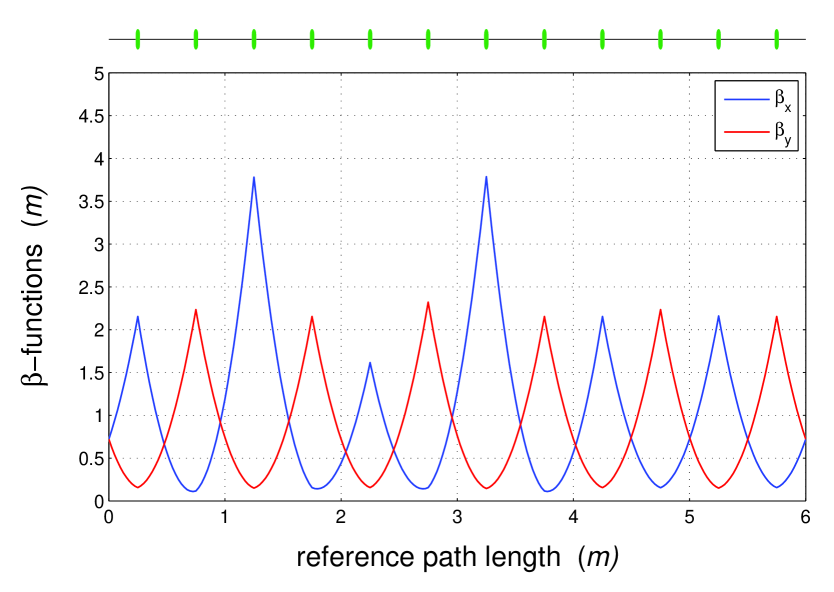
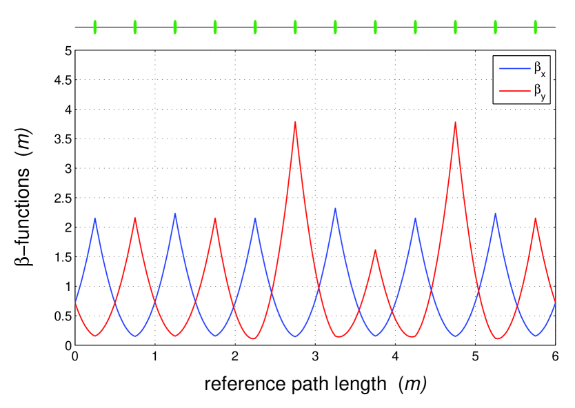
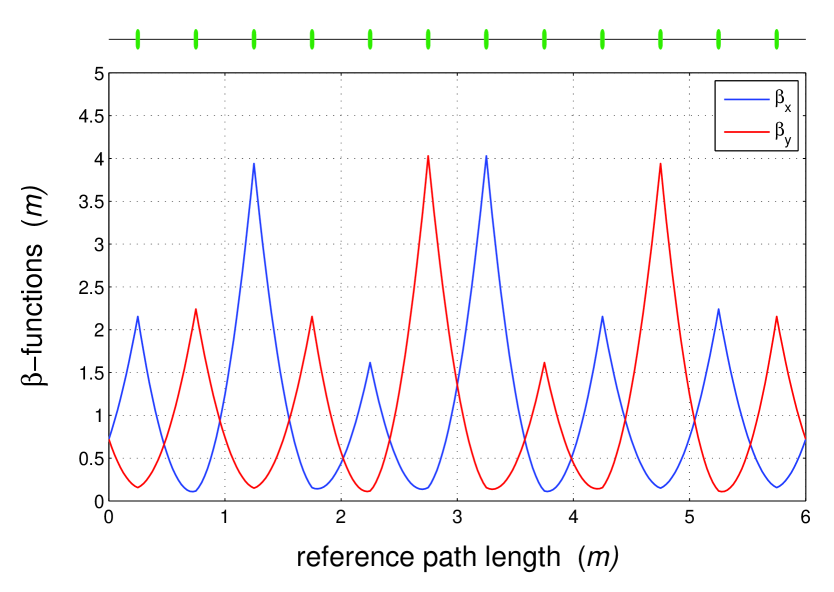
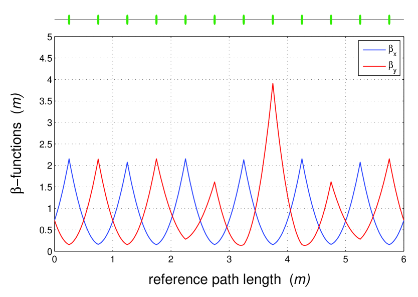
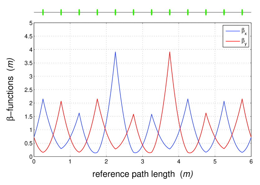
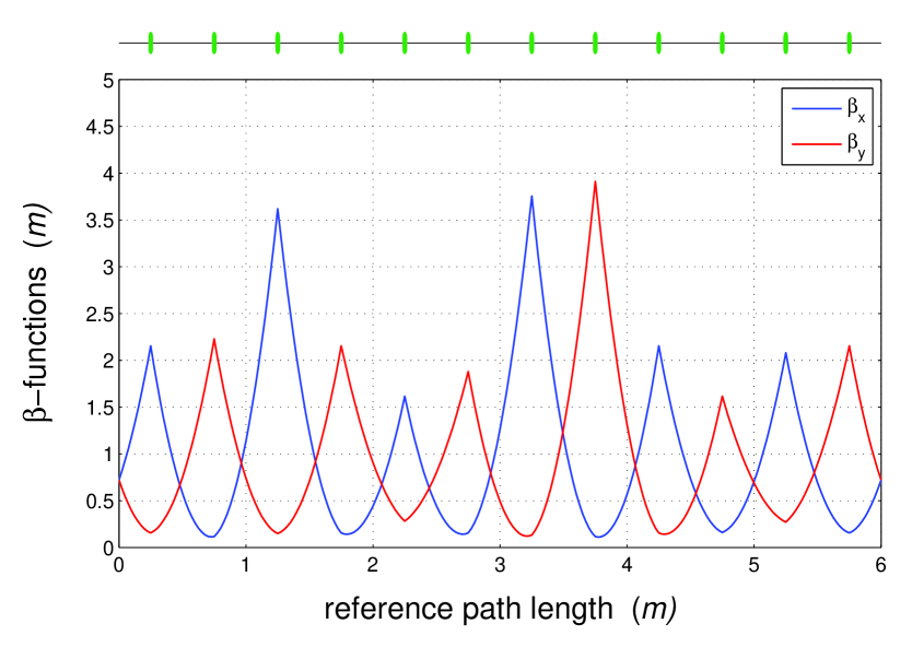
Concerning the changes in the behavior of the betatron functions inside the beam line during the phase scan, then, for example, for all $\,-40^{\circ}\leq\mu_{x,y}\leq 60^{\circ}\,$ the betatron functions $\beta_{x,y}(s)$ in each position $s$ along the beam line satisfy the inequalities

\displaystyle 0.75\,\beta_{min}\,\leq\,\beta_{x,y}(s)\,\leq\,1.88\,\beta_{max},

(228)

where

\displaystyle\beta_{min}\,=\,\frac{2-\sqrt{3}}{\sqrt{3}}\,L,\;\;\;\;\beta_{max}\,=\,\frac{2+\sqrt{3}}{\sqrt{3}}\,L

(229)

are the minimum and the maximum of the periodic FODO solution. In more details the behavior of the betatron functions along the beam line can be seen in Figs. 1-6, where they are drawn for the several values of $\mu_{x,y}$ taken on the borders of the considered area and for the FODO cell length chosen to be one meter.

The presented beam line for the scan of the phase advances is simple, rather elegant and, in the same time, can cover quite a range of phase advances with not very large changes in the lens strengths as compared to their original FODO settings. It can also be adopted to the needs of the European XFEL, where the linac between the two bunch compressors has exactly six FODO cells and two additional quadrupole groups (matching sections) are available at both linac ends.

Note that it is not necessary to keep the periodic matching conditions (206). Any two sets of Twiss parameters can be fixed at the beam line ends, but one has to remember that the choice of them will affect the position of singularities of the solution obtained with the help of the three blocks with decoupled transverse actions. To avoid singularities completely and/or to have additional knob for the control of the betatron functions inside the beam line, one can switch to the solution which utilizes four blocks or to the solution with three blocks plus one additional lens. As described in Sec. IV of this paper, the equal spacing of lenses can also be abandoned, if required.

References

(1) E.Regenstreif, Phase-space transformation by means of quadrupole multiplets, CERN 67-6, March 1967.
(2) E.Regenstreif, Possible and impossible phase-space transformations by means of alternating-gradient doublets and triplets, CERN 67-8, March 1967.
(3) K.L.Brown, R.V.Servranckx, Optics modules for circular accelerator design, NIM A258, 1987.
(4) B.W.Montague, F.Ruggiero, Apochromatic Focusing for Linear Colliders, CLIC-Note 37, May 1987.
(5) B.Zotter, Design considerations for a chromatically corrected final focus for TeV colliders, CLIC-Note 64, June 1988.
(6) O.Napoly, Thin lens telescopes for final focus systems, CERN/LEP-TH/89-69, CLIC Note 102, November 1989.
(7) E.T.d’Amigo, G.Guignard, Analysis of generic insertions made of two symmetric triplets, CERN SL/98-014(AP), May 1998.
(8) T.Roser, Decoupled Beam Line Tuning, AGS/AD/Tech. Note No. 357, January 1992.
(9) N.J.Walker, J.Irwin, M.Woodley, Global Tuning Knobs for the SLC Final Focus, Proceedings of PAC’93, Washington, DC, USA.
(10) D.Cox, J.Little, D.O’Shea, Ideals, Varieties, and Algorithms: An Introduction to Computational Algebraic Geometry and Computer Algebra, Undergraduate Texts in Mathematics. Springer, New York, 1992.
(11) Y-Chiu Chao, J.Irwin, Solution of a three-thin-lens system with arbitrary transfer properties, SLAC-PUB-5834, October 1992.
(12) P.M.Cohn, On the structure of the $GL_{2}$ of a ring, Publ. Math. I.H.E.S., No.30, Paris, p.5-53 (1966).
(13) B.Autin, C.Carli, T.D’Amico, O.Gr $\ddot{\mbox{o}}$ bner, M.Martini, E.Wildner, Beam Optics: A program for analytical beam optics, CERN-98-06, August 1998.
(14) M.Altarelli, R.Brinkmann et al. (Eds), XFEL: The European X-Ray Free-Electron Laser. Technical Design Report, DESY 2006-097, DESY, Hamburg, 2006.

Explicit Thin-Lens Solution for an Arbitrary Four by Four Uncoupled Beam Transfer Matrix

Abstract

I Introduction

II Statement of the problem and preliminary considerations

III Solution of 2D problem using equally spaced thin lenses

III.1 1D problem in terms of PP matrices

III.2 Four-lens block with decoupled transverse actions

III.3 Reduction of 2D problem to two independent or almost independent 1D problems

III.4 Recipe of construction of lens blocks with decoupled transverse actions

IV Generalization to the case of arbitrarily spaced thin lenses

IV.1 Removing of superfluous parameters

Acknowledgements.

Appendix A Elementary matrices and their properties

Appendix B Three Explicit Solutions for Four-Lens Telescopes

B.1 Telescopes which start and end by lens

B.2 Telescopes with equal magnifications in both transverse planes

B.3 Telescopes with nonequal magnifications and special ratio of entrance and exit drifts

Appendix C FODO-Type Beam Line for Independent Scan of Horizontal and Vertical Phase Advances

References

Explicit Thin-Lens Solution
for an Arbitrary Four by Four Uncoupled Beam Transfer Matrix

III.1 1D problem in terms of $P$ matrices