Exploiting Variational Domain-Invariant User Embedding for Partially Overlapped Cross Domain Recommendation
Abstract.
Cross-Domain Recommendation (CDR) has been popularly studied to utilize different domain knowledge to solve the cold-start problem in recommender systems. Most of the existing CDR models assume that both the source and target domains share the same overlapped user set for knowledge transfer. However, only few proportion of users simultaneously activate on both the source and target domains in practical CDR tasks. In this paper, we focus on the Partially Overlapped Cross-Domain Recommendation (POCDR) problem, that is, how to leverage the information of both the overlapped and non-overlapped users to improve recommendation performance. Existing approaches cannot fully utilize the useful knowledge behind the non-overlapped users across domains, which limits the model performance when the majority of users turn out to be non-overlapped. To address this issue, we propose an end-to-end dual-autoencoder with Variational Domain-invariant Embedding Alignment (VDEA) model, a cross-domain recommendation framework for the POCDR problem, which utilizes dual variational autoencoders with both local and global embedding alignment for exploiting domain-invariant user embedding. VDEA first adopts variational inference to capture collaborative user preferences, and then utilizes Gromov-Wasserstein distribution co-clustering optimal transport to cluster the users with similar rating interaction behaviors. Our empirical studies on Douban and Amazon datasets demonstrate that VDEA significantly outperforms the state-of-the-art models, especially under the POCDR setting.
1. Introduction
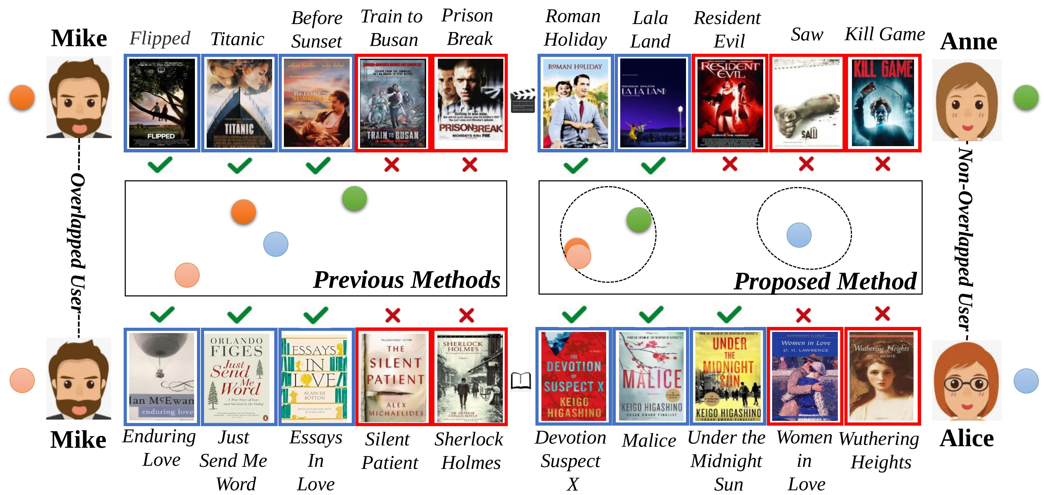
Recommender systems become more and more indispensable in practice since it is a sharp tool for users to easily find what they desire. Nowadays, users always participate in multiple domains (platforms) for different purposes, e.g., buying books on Amazon and watching movies on Youtube. Therefore, Cross Domain Recommendation (CDR) has emerged to utilize both the source and target information for establishing high accuracy recommendation system and overcoming the long-standing data sparsity problem. Most existing CDR models assume the existence of fully overlapped users or items, who have similar tastes or attributions (Dacrema et al., [n. d.]), across domains. For example, a user who likes romantic movies and dislikes horror movies would always like romantic books and dislike horror books as well. Although the movie and book domains are rather different in the specific form of expression, the latent user embedding should properly represent the domain-invariant user personal characteristics such as preferring romantic items and disliking horror items, as shown in Fig. 1. Therefore, existing CDR models can leverage the information from a (source) domain to improve the recommendation accuracy of other (target) domains (Zhu et al., 2021a; Tan et al., 2021). However, in practice, not all users or items are strictly overlapped in CDR settings, which limits the applications of existing CDR approaches.
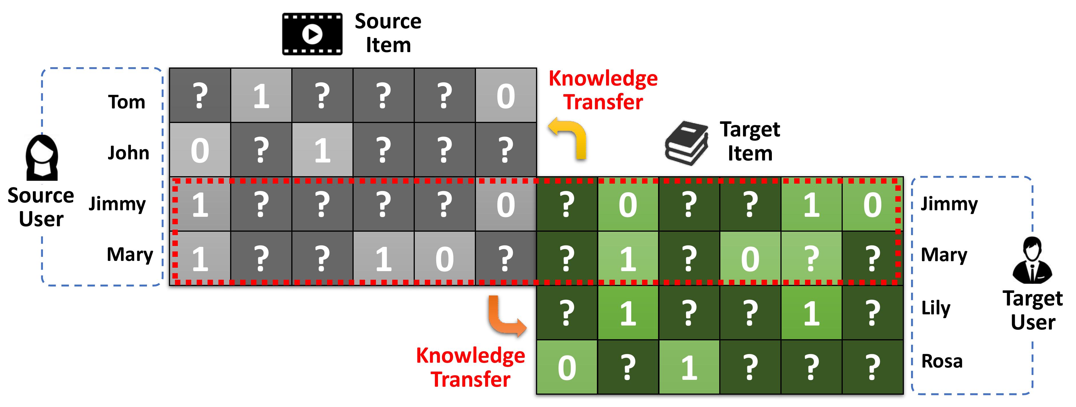
In this paper, we focus on a general problem in CDR based on our observation. That is, two or multiple domains only share a certain degree of overlapped users or items. Specifically, we term this problem as Partially Overlapped Cross Domain Recommendation (POCDR). On the one hand, POCDR has some overlapped users who have rating interactions in both the source and target domains, similar as the conventional CDR problem. On the other hand, POCDR also has several non-overlapped users who only have rating interactions in at most one domain, making it different from the conventional CDR problem. Fig. 2 shows an example of the POCDR problem111Note that the examples and our proposed models in this paper could be easily adapted to the situations where the source and target domains share partially overlapped items. , where Jimmy and Mary are overlapped users, while John, Tom, Lily, and Rosa are non-overlapped users. The prime task of POCDR is to solve the data sparsity problem by leveraging the user-item interactions, with only partially overlapped users across the source and target domains. Solving POCDR is challenging, mainly because it is hard to fully exploit and transfer useful knowledge across domains, especially when extremely few users are overlapped.
Existing researches on CDR cannot solve the POCDR problem well. Firstly, conventional CDR approaches can only adjust to the circumstances where the majority of users are overlapped, but they cannot maintain the prediction performance when the majority of users turn out to be non-overlapped. The overlapped users can be utilized as a bridge to transfer knowledge across domains, while knowledge of the non-overlapped users cannot be extracted efficiently, which leads to unreliable predictions. Secondly, there exist non-overlapped CDR models which could adopt group-level codebook transfer to provide recommendation (Li et al., 2009a, b). However, they cannot ensure that the shared embedding information across domains is consistent, which limits the effectiveness of knowledge transfer (Zhang et al., 2018). Take the toy example shown in the left of Fig. 1 for example, lacking effective constraint on the non-overlapped users leads to the consequence that Alice who likes horror but dislikes romantic has the nearest embedding distance with Mike who likes romantic but dislikes horror instead. Obviously, insufficient training of the non-overlapped users finally will deteriorate the model performance. Meanwhile, conventional CDR approaches have concluded that clustering the overlapped users with similar characteristics can also promote the model performance (Wang et al., 2019a; Farseev et al., 2017). However, how to properly co-cluster similar overlapped and non-overlapped users across domains is still a serious challenge in POCDR setting. In a nutshell, current CDR models cannot achieve satisfying performance because of the lacking of sufficient techniques to fully leverage the data in both domains under the POCDR setting.
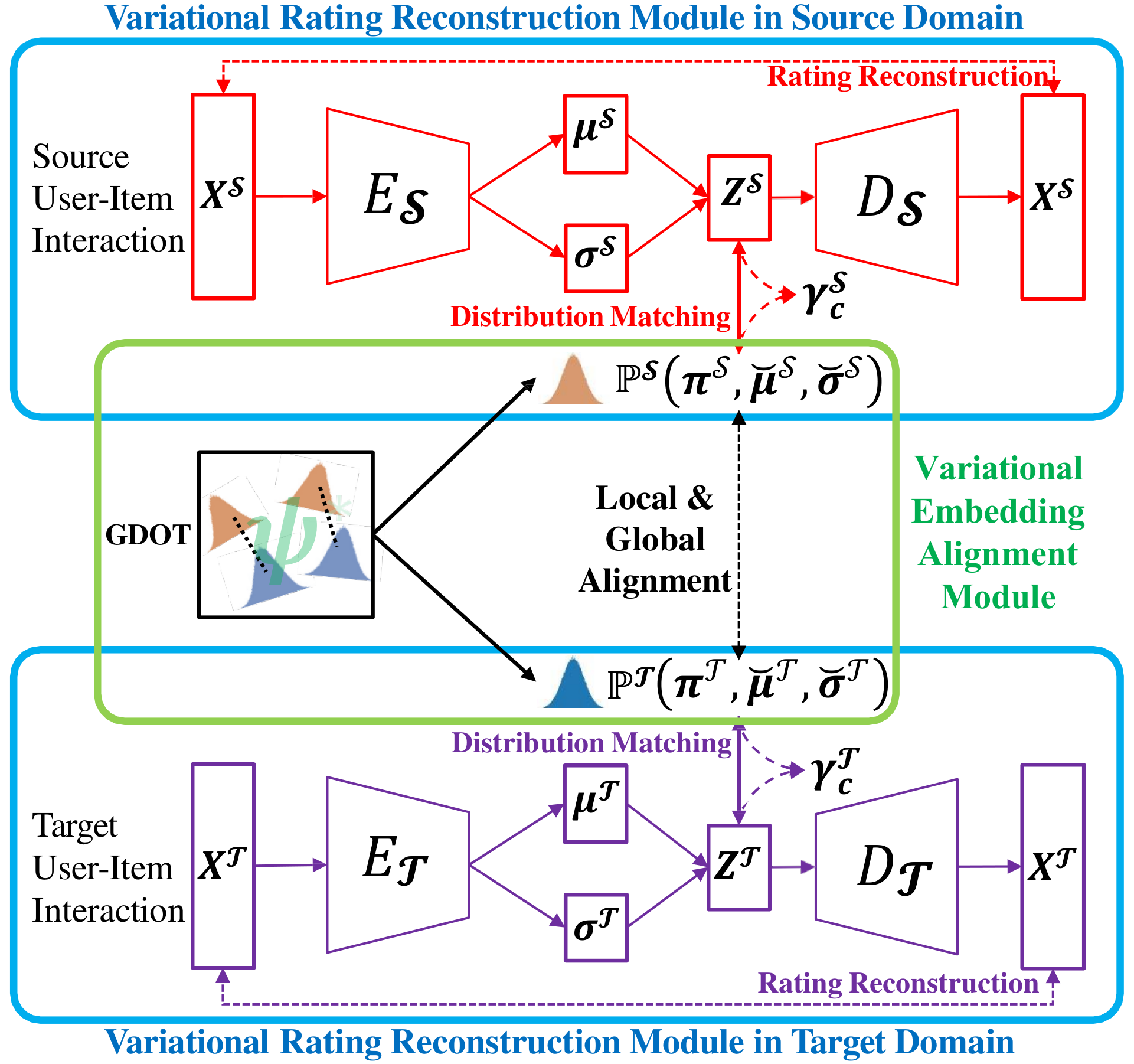
To address the aforementioned issue, in this paper, we propose VDEA, an end-to-end dual-autoencoder with Variational Domain-invariant Embedding Alignment (VDEA), for solving the POCDR problem. The core insight of VDEA is exploiting domain-invariant embedding across different domains, for both the overlapped and non-overlapped users. Again, in the example of Fig.1, Mike and Anne who share similar tastes, i.e., preferring romantic items rather than horror ones, should have similar domain-invariant embeddings. In contrast, users with different tastes, e.g., Mike and Alice, should be pushed away in the latent embedding space. In order to better represent user embedding with high-quality rating prediction and knowledge transfer ability, we utilize two modules in VDEA, i.e., variational rating reconstruction module and variational embedding alignment module, as will be shown in Fig. 3. On the one hand, the variational rating reconstruction module aims to capture user collaborative preferences in the source and target domains with cross-entropy loss. On the other hand, the variational rating reconstruction module can cluster users with similar tastes or characteristics on Mixture-Of-Gaussian distribution simultaneously. The variational embedding alignment module further includes two main components, e.g, variational local embedding alignment and variational global embedding alignment. Variational local embedding alignment tends to match the overlapped users across domains to obtain more expressive user embeddings. Variational global embedding alignment can co-cluster the similar user groups via distribution optimal transport, transferring useful knowledge among both overlapped and non-overlapped users. By doing this, we can not only obtain discriminative domain-invariant user embedding in a single domain, but also cluster users with similar preferences between the source and target domains.
We summarize our main contributions as follows: (1) We propose a novel framework, i.e., VDEA, for the POCDR problem, which can utilize the rating interactions of both overlapped and non-overlapped users to improve the recommendation performance. (2) In order to better exploit users with similar tastes or characteristics, we equip VDEA with variational inference and distribution co-clustering optimal transport to obtain more discriminative and domain-invariant latent user embedding. (3) Extensive empirical studies on Douban and Amazon datasets demonstrate that VDEA significantly improves the state-of-the-art models, especially under the POCDR setting.
2. Related Work
Cross Domain Recommendation. Cross Domain Recommendation (CDR) emerges as a technique to alleviate the long-standing data sparsity problem in recommendation by assuming the same user set across domains (Li et al., 2009a; Weike et al., 2013; Liu et al., 2022; Tan et al., 2022). According to (Zhu et al., 2021a), existing CDR models have three main types, i.e., transfer-based methods, clustered-based methods, and multitask-based methods. Transfer-based methods (Zhao et al., 2020; Man et al., 2017) learn a linear or nonlinear mapping function across domains. Some recent method (Chen et al., 2020b) even adopts equivalent transformation to obtain more reliable knowledge across domains with shared users. Clustered-based methods (Wang et al., 2019b) adopt the co-clustering approach to learn cross-domain comprehensive embeddings by collectively leveraging single-domain and cross-domain information within a unified framework. Multi-task-based methods (Hu et al., 2018; Zhu et al., 2019, 2021b) enable dual knowledge transfer across domains by introducing shared connection modules in neural networks. However, the majority of current CDR frameworks have the underlying assumption that the source and target domains share the same set of users or items (Zhu et al., 2021a). Conventional CDR approaches cannot perfectly solve the POCDR problem where a large number of users are non-overlapped. As a comparison, in this paper, we focus on the POCDR problem, and propose VDEA which adopt variational local and global embedding alignment for better exploiting domain-invariant embeddings for all the users across domains.
Domain Adaptation. Domain adaptation aims to transfer useful knowledge from the source samples with labels to target samples without labels for enhancing the target performance. Existing work on this is mainly of three types, i.e., discrepancy-based methods (Pan et al., 2011; Borgwardt et al., 2006), adversarial-based methods (Ganin et al., 2016; Long et al., 2017), and reconstruction-based methods (Zhuang et al., 2021; Tan et al., 2018). Discrepancy-based methods, e.g., Maximum Mean Discrepancy (MMD) (Borgwardt et al., 2006), Correlation Alignment (CORAL). Recently, ESAM (Chen et al., 2020a) extends CORAL with attribution alignment for solving the long-tailed item recommendation problem. Adversarial-based methods integrate a domain discriminator for adversarial training, including Domain Adversarial Neural Network (DANN) (Ganin et al., 2016) and Adversarial Discriminative Domain Adaptation (ADDA) (Tzeng et al., 2017). DARec (Yuan et al., 2019) even transferred knowledge across domains with shared users via deep adversarial adaptation technique. Reconstruction based methods utilize autoencoder to exploit the domain-invariant latent representations, e.g., Unsupervised Image-to-Image Translation Networks (UNIT) (Liu et al., 2017; Huang et al., 2018), which indicates that exploiting shared latent space across different domains can enhance the model performance and generalization. However, most existing reconstruction-based models fail to adopt a dual discriminator network to reduce the distribution discrepancy across different domains. In this paper, we propose to combine reconstruction-based model with discrepancy-based method for better exploiting domain-invariant embeddings.
3. Modeling for VDEA
3.1. Framework of VDEA
First, we describe notations. We assume there are two domains, i.e., a source domain and a target domain . We assume has users and items, and has users and items. Unlike conventional cross domain recommendation, in POCDR, the source and target user sets are not completely the same. We use the overlapped user ratio to measure how many users are concurrence. Bigger means more overlapped users across domains, while smaller means the opposite situation.
Then, we introduce the overview of our proposed VDEA framework. The aim of VDEA is providing better single domain recommendation performance by leveraging useful cross domain knowledge for both overlapped and non-overlapped users. VDEA model mainly has two modules, i.e., variational rating reconstruction module and variational embedding alignment module, as shown in Fig. 3. The variational rating reconstruction module establishes user embedding according to the user-item interactions on the source and target domains. Meanwhile, the variational rating reconstruction module also clusters the users with similar characteristics or preferences based on their corresponding latent embeddings to enhance the model generalization. The basic intuition is that users with similar behaviors should have close embedding distances through this module with deep unsupervised clustering approach (Wang et al., 2019a; Ma et al., 2019; Wang et al., 2019b). The variational embedding alignment module has two parts, i.e., variational local embedding alignment and variational global embedding alignment, sufficiently aligning the local and global user embeddings across domains. The local embedding alignment can utilize the user-item ratings of the overlapped users to obtain more expressive user embeddings (Krafft and Schmitz, 1969). Intuitively, expressive overlapped user embedding can enhance model training of the non-overlapped users, since the non-overlapped users share the similar preference (e.g., romantic or realistic) as the overlapped ones (Zhang et al., 2018). Moreover, the global embedding alignment can also directly co-cluster both the overlapped and non-overlapped users with similar tastes, which can boost the procedure of knowledge transfer. To this end, the variational embedding alignment module can exploit domain-invariant latent embeddings for both overlapped and non-overlapped users. The framework of VDEA is demonstrated in Fig. 3 and we will introduce its two modules in details later.
3.2. Variational Rating Reconstruction Module
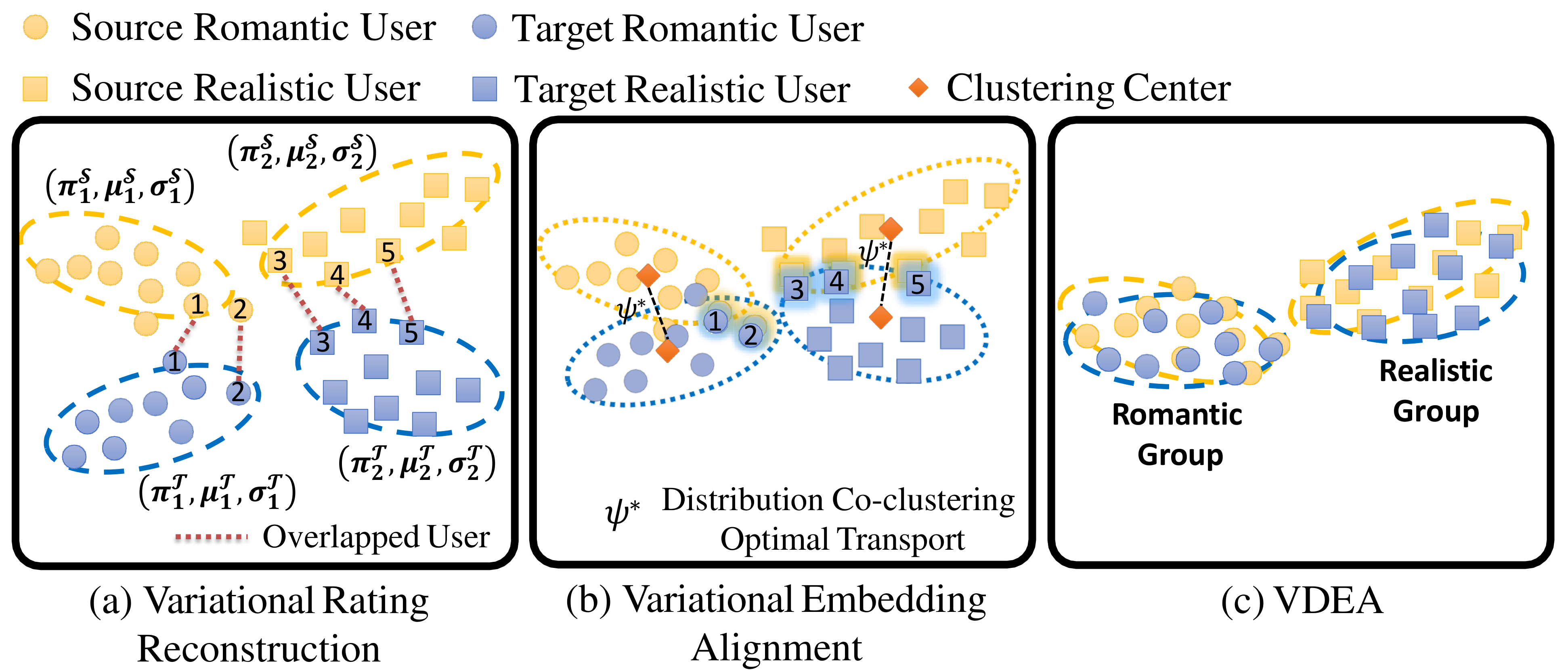
To begin with, we first introduce the variational rating reconstruction module. We define and as the user-item interactions on the source and target domains respectively, and is batch size. We adopt dual variational autoencoder as the main architecture for accurately representing and clustering user embedding according to the rating interactions. We utilize two variational autoenocers in VDEA, i.e., a source variational autoencoder and a target variational autoencoder, for source and target domains, respectively. The source variational autoencoder includes the encoder and decoder . Similarly, the target variational autoencoder includes the encoder and decoder . The encoders and can predict the mean ( and ) and log variance ( and ) for the input data as and . In order to guarantee gradient descent in back propagation, we also apply the reparamaterize mechanism (Liang et al., 2018; Shenbin et al., 2020) as and , where are randomly sampled from normal distribution, and , and have the same dimension . Inspired by variational deep embedding (Jiang et al., 2016), we expect the latent user embedding conform to Mixture-Of-Gaussian distribution for grouping similar users. The dual variational autoencoder also reconstructs the user-item interaction as and . In this section, we will first present the variational evidence lower bound according to the Mixture-Of-Gaussian distributions, and then illustrate the rating reconstruction and distribution matching for the total loss. By proposing the variational rating reconstruction module, the users with similar characteristics will be clustered in each domain, as can be seen in Fig. 4(a).
Variational evidence lower bound. Since we tend to cluster the users with similar preferences, we choose Mixture-Of-Gaussian as the user latent distribution. To do this, we let user embedding obey the Mixture-Of-Gaussian distribution and properly predict the user-item rating interactions through variational evidence lower bound (Jiang et al., 2016). The variational evidence lower bound for the variational rating reconstruction module is to maximize the likelihood of the given user embeddings in Mixture-Of-Gaussian distribution. Specifically, we define the prior source and target latent distributions as and respectively, where denotes the distribution of Mixture-Of-Gaussian. and denote the prior probability of each cluster components in Mixture-Of-Gaussian, and denote the mean and variance of the Gaussian distribution in the source domain and target domain, respectively. For the -th user, with denoting the total number of clusters. Taking the joint probability in the source domain for example, it can be factorized as in the perspective of the generative process:
| (1) | ||||
where is the observed sample and is the latent user embedding. The corresponding cluster is with denoting the prior categorical distribution. and denote the mean and variance of the Gaussian distribution to the -th cluster. denotes multivariate Bernoulli distribution for the output of the decoder.
We then adopt Jensen’s inequality with the mean-field assumption to estimate the Evidence Lower Bound (ELBO) by maximizing . Following (Jiang et al., 2016), ELBO can be rewritten in a simplified form as:
| (2) | ||||
where the first term represents the rating reconstruction loss that encourages the model to fit the user-item interactions well. The second term calculates the Kullback-Leibler divergence between Mixture-of-Gaussians prior and the variational posterior . Furthermore, in order to balance the reconstruction capacity (the first term) efficiently and disentangle the latent factor (the second term) automatically, we change the KL divergence into the following optimization equation with constraints:
| (3) | ||||
where specifies the strength of the KL constraint. Rewriting the optimization problem in Equation (LABEL:equ:opt) under the KKT conditions and neglecting the small number of , we have:
| (4) | ||||
where denotes the hyper-parameter between rating modelling and latent distribution matching (Higgins et al., 2016).
Loss computing. The loss of the variational rating reconstruction module can be deduced from ELBO, which has two main parts, i.e., rating reconstruction and distribution matching. For the rating reconstruction part, the reconstruction loss is given as below:
| (5) |
where is the cross-entropy loss. For the distribution matching part, it can be further substituted through Kullback-Leibler divergence calculation as below:
| (6) | ||||
where represents the probability of belonging to the -th cluster and it can be formulated as:
| (7) |
By the detailed process on the source domain through maximizing ELBO w.r.t. the parameters of , the latent user embeddings will be clustered and become much more discriminative. Likewise, we can also optimize ELBO on the target domain parameters . Therefore, the loss of the whole variational rating reconstruction module is given as:
| (8) | ||||
3.3. Variational Embedding Alignment Module
As we have motivated before, the embeddings of similar users should be clustered through variational deep embedding to make them more discriminative, as is shown in Fig. 4. However, how to align these Mixture-Of-Gaussian distribution across domains remains a tough challenge. In order to tackle this issue, we propose variational embedding alignment from both local and global perspectives.
Variational local embedding alignment. Variational local embedding alignment in VDEA aims to align the corresponding overlapped user embedding distribution across domains. Since variational encoder can measure the mean and variance of the input data, we adopt the 2-Wasserstein distance of different Gaussians distributions to calculate the variational local user embedding alignment loss:
| (9) | ||||
where denotes the 2-Wasserstein distance of different Gaussians distributions that measures the discrepancy across domains, indicates whether a user occurs simultaneously in both domains under the POCDR setting, means the -th user in the source domain has the same identification with the -th user in the target domain, otherwise . The distribution estimation can further help the model to better capture the uncertainties of the learned embeddings (Truong et al., 2021).
Variational global embedding alignment. VDEA should also align the global distributions of both the overlapped and non-overlapped users across domains. Similar intra-domain users can be clustered through variational local embedding alignment, however, there is still a distribution discrepancy between the source and target domains. Thus, how to match the whole user distributions across domains without explicit label information remains the key issue.
In order to obtain the alignment results effectively, we propose the Gromov-Wasserstein Distribution Co-Clustering Optimal Transport (GDOT) approach. Unlike conventional optimal transport (Santambrogio, 2015; Villani, 2008) that only aligns user embeddings, our proposed GDOT for domain adaptation performs user embedding distribution alignment in the source and target domains. The optimization of optimal transport is based on the Kantorovich problem (Angenent et al., 2003), which seeks a general coupling between and :
| (10) |
where denotes the latent embedding probability distribution between and . The cost function matrix measures the difference between each pair of distributions. To facilitate calculation, we formulate the discrete optimal transport formulation as , where is the ideal coupling matrix between the source and target domains, representing the joint probability of the source probability and the target probability . The matrix denotes a pairwise Gaussian distribution distance among the source probability and target probability as:
| (11) |
Meanwhile denotes the tensor matrix multiplication, which means . The second term is a regularization term and is a balance hyper parameter. The matching matrix follows the constraints that with denoting the number of clusters. We apply the Sinkhorn algorithm (Cuturi, 2013; Xu et al., 2020) for solving the optimization problem by adopting the Lagrangian multiplier to minimize the objective function as below:
| (12) |
where and are both Lagrangian multipliers. We first randomly generate a matrix that meets the boundary constraints and then define the variable . Taking the differentiation of Equation (12) on variable , we can obtain:
| (13) |
Taking Equation (13) back to the original constraints and , we can obtain that:
| (14) |
Since we define , , and . Through iteratively solving Equation (14) on the variables and , we can finally obtain the coupling matrix on Equation (13). We show the iteration optimization scheme of GDOT in Algorithm 1. In summary, variational embedding alignment can obtain the optimal transport solution as for each corresponding sub-distribution, as shown with dot lines in Fig. 4(b).
After that, the variational global embedding alignment loss is given as:
| (15) |
The bigger for the matching constraint, the closer between the distributions and .
3.4. Putting Together
The total loss of VDEA could be obtained by combining the losses of the variational rating reconstruction module and the variational embedding alignment module. That is, the losses of VDEA is given as:
| (16) |
where and are hyper-parameters to balance different type of losses. By doing this, users with similar rating behaviors will have close embedding distance in single domain through the variational inference, and the user embeddings across domains will become domain-invariant through GDOT which has been shown in Fig. 4(c).
4. Empirical Study
In this section, we conduct experiments on several real-world datasets to answer the following questions: (1) RQ1: How does our approach perform compared with the state-of-the-art single-domain or cross-domain recommendation methods? (2) RQ2: How do the local and global embedding alignments contribute to performance improvement? Can proposed GDOT better align the global distribution? (3) RQ3: How does the performance of VDEA vary with different values of the hyper-parameters?
4.1. Datasets and Tasks
We conduct extensive experiments on two popularly used real-world datasets, i.e., Douban and Amazon, for evaluating our models on POCDR tasks (Zhu et al., 2019, 2021b; Ni et al., 2019). First, the Douban dataset (Zhu et al., 2019, 2021b) has two domains, i.e., Book and Movie, with user-item ratings. Second, the Amazon dataset (Zhao et al., 2020; Ni et al., 2019) has four domains, i.e., Movies and TV (Movie), Books (Book), CDs and Vinyl (Music), and Clothes (Clothes). The detailed statistics of these datasets after pre-process will be shown in Table 1. For both datasets, we binarize the ratings to 0 and 1. Specifically, we take the ratings higher or equal to 4 as positive and others as 0. We also filter the users and items with less than 5 interactions, following existing research (Yuan et al., 2019; Zhu et al., 2021b). We provide four main tasks to evaluate our model, i.e., Amazon Movie Amazon Music, Amazon Movie Amazon Book, Amazon Movie Amazon Clothes, and Douban Movie Douban Book. It is noticeable that some tasks are rather simple because the source and target domains are similar, e.g., Amazon Movie Amazon Book, while some tasks are difficult since these two domains are different, e.g., Amazon Movie Amazon Clothes (Yu et al., 2020).
| Datasets | Users | Items | Ratings | Density | |
|---|---|---|---|---|---|
| Amazon | Movie | 15,914 | 17,794 | 416,228 | 0.14% |
| Music | 20,058 | 280,398 | 0.09% | ||
| Amazon | Movie | 29,476 | 24,091 | 591,258 | 0.08% |
| Book | 41,884 | 579,131 | 0.05% | ||
| Amazon | Movie | 13,267 | 20,433 | 216,868 | 0.08% |
| Clothes | 21,054 | 195,550 | 0.07% | ||
| Douban | Movie | 2,106 | 9,551 | 871,280 | 4.33% |
| Book | 6,766 | 90,164 | 0.63% | ||
4.2. Experimental Settings
We randomly divide the observed source and target data into training, validation, and test sets with a ratio of 8:1:1. Meanwhile, we vary the overlapped user ratio in . Different user overlapped ratio represents different situations, e.g., represents only few users are overlapped while means most of users are overlapped (Zhang et al., 2018). For all the experiments, we perform five random experiments and report the average results. We choose Adam (Kingma and Ba, 2014) as optimizer, and adopt Hit Rate (HR) and NDCG (Wang et al., 2019c) as the ranking evaluation metrics with .
| (Amazon) Movie & Music | (Amazon) Movie & Clothes | ||||||||||||
| Movie | Music | Movie | Music | Movie | Music | Movie | Clothes | Movie | Clothes | Movie | Clothes | ||
| KerKT | HR | 0.3463 | 0.3505 | 0.3750 | 0.3936 | 0.4228 | 0.4409 | 0.2155 | 0.0876 | 0.2614 | 0.1165 | 0.3155 | 0.1648 |
| NDCG | 0.2504 | 0.2572 | 0.2858 | 0.2994 | 0.3253 | 0.3352 | 0.1423 | 0.0983 | 0.1867 | 0.1285 | 0.2425 | 0.1676 | |
| NeuMF | HR | 0.3661 | 0.3722 | 0.3987 | 0.4128 | 0.4467 | 0.4661 | 0.2281 | 0.0990 | 0.2697 | 0.1382 | 0.3307 | 0.1820 |
| NDCG | 0.2602 | 0.2686 | 0.2944 | 0.3109 | 0.3319 | 0.3488 | 0.1606 | 0.1081 | 0.1980 | 0.1361 | 0.2570 | 0.1774 | |
| MultVAE | HR | 0.3807 | 0.3861 | 0.4019 | 0.4247 | 0.4526 | 0.4768 | 0.2373 | 0.1047 | 0.2802 | 0.1435 | 0.3451 | 0.1890 |
| NDCG | 0.2654 | 0.2758 | 0.2995 | 0.3346 | 0.3372 | 0.3649 | 0.1686 | 0.1161 | 0.2084 | 0.1490 | 0.2627 | 0.1868 | |
| BiVAE | HR | 0.3880 | 0.3956 | 0.4104 | 0.4392 | 0.4621 | 0.4833 | 0.2436 | 0.1152 | 0.2934 | 0.1627 | 0.3553 | 0.1991 |
| NDCG | 0.2754 | 0.2836 | 0.3109 | 0.3365 | 0.3417 | 0.3758 | 0.1817 | 0.1266 | 0.2218 | 0.1615 | 0.2754 | 0.1989 | |
| DARec | HR | 0.3831 | 0.3898 | 0.4055 | 0.4311 | 0.4560 | 0.4779 | 0.2414 | 0.1084 | 0.2878 | 0.1509 | 0.3505 | 0.1940 |
| NDCG | 0.2699 | 0.2740 | 0.3038 | 0.3386 | 0.3423 | 0.3689 | 0.1754 | 0.1216 | 0.2162 | 0.1565 | 0.2697 | 0.1973 | |
| ETL | HR | 0.3893 | 0.4002 | 0.4160 | 0.4434 | 0.4629 | 0.4858 | 0.2508 | 0.1160 | 0.3019 | 0.1683 | 0.3632 | 0.2057 |
| NDCG | 0.2751 | 0.2898 | 0.3145 | 0.3393 | 0.3455 | 0.3781 | 0.1872 | 0.1294 | 0.2295 | 0.1720 | 0.2818 | 0.2036 | |
| DML | HR | 0.3941 | 0.4064 | 0.4182 | 0.4510 | 0.4676 | 0.4885 | 0.2552 | 0.1201 | 0.3093 | 0.1714 | 0.3674 | 0.2065 |
| NDCG | 0.2763 | 0.2954 | 0.3156 | 0.3425 | 0.3487 | 0.3778 | 0.1926 | 0.1335 | 0.2349 | 0.1672 | 0.2861 | 0.2050 | |
| VDEA | HR | 0.4404 | 0.4457 | 0.4602 | 0.4865 | 0.4956 | 0.5148 | 0.2867 | 0.1485 | 0.3342 | 0.1944 | 0.3884 | 0.2303 |
| NDCG | 0.3021 | 0.3207 | 0.3322 | 0.3645 | 0.3659 | 0.3966 | 0.2231 | 0.1589 | 0.2538 | 0.1869 | 0.2973 | 0.2287 | |
| (Amazon) Movie & Book | (Douban) Movie & Book | ||||||||||||
| Movie | Book | Movie | Book | Movie | Book | Movie | Book | Movie | Book | Movie | Book | ||
| KerKT | HR | 0.3507 | 0.3534 | 0.3903 | 0.3958 | 0.4448 | 0.4421 | 0.4518 | 0.3009 | 0.5094 | 0.3353 | 0.5496 | 0.3657 |
| NDCG | 0.2505 | 0.2559 | 0.2947 | 0.3013 | 0.3266 | 0.3358 | 0.2529 | 0.1392 | 0.3171 | 0.1705 | 0.3324 | 0.2006 | |
| NeuMF | HR | 0.3722 | 0.3774 | 0.4155 | 0.4183 | 0.4607 | 0.4656 | 0.4610 | 0.3253 | 0.5247 | 0.3526 | 0.5659 | 0.3881 |
| NDCG | 0.2638 | 0.2672 | 0.3021 | 0.3094 | 0.3356 | 0.3457 | 0.2656 | 0.1450 | 0.3291 | 0.1763 | 0.3523 | 0.2082 | |
| MultVAE | HR | 0.3878 | 0.3940 | 0.4239 | 0.4217 | 0.4682 | 0.4751 | 0.4793 | 0.3503 | 0.5312 | 0.3864 | 0.5780 | 0.4044 |
| NDCG | 0.2763 | 0.2728 | 0.3124 | 0.3108 | 0.3440 | 0.3539 | 0.2745 | 0.1627 | 0.3441 | 0.1952 | 0.3724 | 0.2163 | |
| BiVAE | HR | 0.3983 | 0.3992 | 0.4426 | 0.4501 | 0.4837 | 0.4851 | 0.4921 | 0.3619 | 0.5586 | 0.4208 | 0.6014 | 0.4393 |
| NDCG | 0.2852 | 0.2837 | 0.3289 | 0.3324 | 0.3520 | 0.3613 | 0.2945 | 0.1728 | 0.3664 | 0.2326 | 0.3935 | 0.2437 | |
| DARec | HR | 0.3947 | 0.3918 | 0.4364 | 0.4350 | 0.4748 | 0.4795 | 0.4859 | 0.3538 | 0.5445 | 0.3918 | 0.5912 | 0.4251 |
| NDCG | 0.2816 | 0.2783 | 0.3230 | 0.3297 | 0.3484 | 0.3572 | 0.2797 | 0.1668 | 0.3563 | 0.2035 | 0.3819 | 0.2286 | |
| ETL | HR | 0.4022 | 0.4075 | 0.4269 | 0.4538 | 0.4883 | 0.4905 | 0.5044 | 0.3706 | 0.4269 | 0.4538 | 0.6175 | 0.4503 |
| NDCG | 0.2959 | 0.2893 | 0.3341 | 0.3386 | 0.3590 | 0.3724 | 0.3088 | 0.1817 | 0.3715 | 0.2314 | 0.3992 | 0.2496 | |
| DML | HR | 0.4070 | 0.4013 | 0.4522 | 0.4557 | 0.4932 | 0.4941 | 0.5187 | 0.3725 | 0.5805 | 0.4298 | 0.6284 | 0.4618 |
| NDCG | 0.3073 | 0.2934 | 0.3389 | 0.3426 | 0.3642 | 0.3716 | 0.3176 | 0.1884 | 0.3785 | 0.2332 | 0.4025 | 0.2551 | |
| VDEA | HR | 0.4481 | 0.4342 | 0.4813 | 0.4824 | 0.5145 | 0.5058 | 0.5662 | 0.4023 | 0.6009 | 0.4345 | 0.6435 | 0.4709 |
| NDCG | 0.3338 | 0.3206 | 0.3581 | 0.3612 | 0.3889 | 0.3857 | 0.3519 | 0.2150 | 0.3903 | 0.2421 | 0.4207 | 0.2644 | |
4.3. Baseline
We compare our proposed VDEA with the following state-of-the-art cross domain recommendation models. (1) KerKT (Zhang et al., 2018) Kernel-induced knowledge transfer for overlapping entities (KerKT) which is the first attempt on POCDR problem. It uses a shallow model with multiple steps to model and align user representations. (2) NeuMF (He et al., 2017) Neural Collaborative Filtering for Personalized Ranking (NeuMF) replaces the traditional inner product with a neural network to learn an arbitrary function on the single domain accordingly. (3) MultVAE (Liang et al., 2018) Variational Autoencoders for Collaborative Filtering (MultVAE) extends variational autoencoders for recommendation. (4) BiVAE (Truong et al., 2021) Bilateral Variational Autoencoder for Collaborative Filtering (BiVAE) further adopts variational autoencoder on both user and item to model the rating interactions. (5) DARec (Yuan et al., 2019) Deep Domain Adaptation for Cross-Domain Recommendation via Transferring Rating Patterns (DARec) adopts adversarial training strategy to extract and transfer knowledge patterns for shared users across domains. (6) ETL (Chen et al., 2020b) Equivalent Transformation Learner (ETL) of user preference in CDR adopts equivalent transformation module to capture both the overlapped and domain-specific properties. (7) DML (Li and Tuzhilin, 2021) Dual Metric Learning for Cross-Domain Recommendations (DML) is the recent state-of-the-art CDR model which transfers information across domains based on dual modelling.
4.4. Implementation Details
We set batch size for both the source and target domains. The latent embedding dimension is set to . We assume both source and target users share the same embedding dimension according to previous research (Liu et al., 2017; Chen et al., 2020b). For the variational rating reconstruction module, we adopt the heuristic strategy for selecting the disentangle factor by starting from and gradually increasing to through KL annealing (Liang et al., 2018). Empirically, we set the cluster number as . Meanwhile, we set hyper-parameters for Gromov-Wasserstein Distribution Co-Clustering Optimal Transport. For VDEA model, we set the balance hyper-parameters as and .
| (Amazon) Movie & Music | (Amazon) Movie & Book | (Amazon) Movie & Clothes | |||||||||||
| Movie | Music | Movie | Music | Movie | Book | Movie | Book | Movie | Clothes | Movie | Clothes | ||
| VDEA-Base | HR | 0.3901 | 0.3994 | 0.4597 | 0.4822 | 0.3895 | 0.4002 | 0.4816 | 0.4789 | 0.2467 | 0.1169 | 0.3613 | 0.1944 |
| NDCG | 0.2710 | 0.2805 | 0.3368 | 0.3723 | 0.2816 | 0.2862 | 0.3485 | 0.3591 | 0.1826 | 0.1245 | 0.2703 | 0.1938 | |
| VDEA-Local | HR | 0.4217 | 0.4238 | 0.4854 | 0.5034 | 0.4295 | 0.4305 | 0.5037 | 0.4965 | 0.2718 | 0.1373 | 0.3779 | 0.2194 |
| NDCG | 0.2889 | 0.3076 | 0.3561 | 0.3850 | 0.3219 | 0.3158 | 0.3787 | 0.3793 | 0.2084 | 0.1497 | 0.2864 | 0.2198 | |
| VDEA-Global | HR | 0.4330 | 0.4315 | 0.4913 | 0.5082 | 0.4386 | 0.4277 | 0.5092 | 0.5017 | 0.2786 | 0.1402 | 0.3826 | 0.2259 |
| NDCG | 0.2936 | 0.3134 | 0.3614 | 0.3901 | 0.3274 | 0.3129 | 0.3816 | 0.3822 | 0.2145 | 0.1510 | 0.2916 | 0.2231 | |
| VDEA | HR | 0.4404 | 0.4456 | 0.4956 | 0.5147 | 0.4481 | 0.4342 | 0.5145 | 0.5058 | 0.2867 | 0.1485 | 0.3884 | 0.2303 |
| NDCG | 0.3021 | 0.3207 | 0.3659 | 0.3966 | 0.3338 | 0.3206 | 0.3889 | 0.3857 | 0.2231 | 0.1589 | 0.2973 | 0.2287 | |
4.5. Recommendation Performance (for RQ1)
The comparison results on Douban and Amazon datasets are shown in Table 1. From them, we can find that: (1) With the decrease of the overlapped user ratio , the performance of all the models will also decrease. This phenomenon is reasonable since fewer overlapped users may raise the difficulty of knowledge transfer across different domains. (2) The conventional shallow model KerKT with multiple separated steps cannot model the complex and nonlinear user-item relationship under the POCDR setting. (3) Most of the cross domain recommendation models (e.g., DML) perform better than single domain recommendation model (e.g., NeuMF), indicating that cross domain recommendation can integrate more useful information to enhance the model performance, which is always conform to our common sense. (4) Although ETL and DML can get reasonable results on conventional cross domain recommendation problem where two domains are highly overlapped, it cannot achieve satisfied solutions on the general POCDR problem. When the majority of users are non-overlapped, ETL and DML cannot fully utilize the knowledge transfer from the source domain to the target domain and thus lead to model degradation. The main reason is that their loss functions only act on the overlapped users without considering the non-overlapped users. The same phenomenon happens on other baseline models, e.g., DARec. (5) VDEA with deep latent embedding clustering can group users with similar behaviors and can further enhance the performance under the POCDR settings. We also observe that our proposed VDEA can also have great prediction improvement even when the overlapped user ratio is much smaller (e.g., ). Meanwhile our proposed VDEA still obtains better results when the source and target domains are different (e.g., Amazon Movie Amazon Clothes) which indicates the high efficacy of VDEA.
4.6. Analysis (for RQ2 and RQ3)
Ablation. To study how does each module of VDEA contribute to the final performance, we compare VDEA with its several variants, including VDEA-Base, VDEA-Local, and VDEA-Global. (1) VDEA-Base only includes the variational rating reconstruction loss , that is . (2) VDEA-Local excludes global embedding alignment for user embedding, that is . (3) VDEA-Global adopts local embedding alignment while utilizing the adversarial domain alignment method in DARec for the global embedding alignment. The comparison results are shown in Table 3. From it, we can observe that: (1) VDEA-Base can already achieve good results compared with some other models (e.g., MultVAE), indicating that clustering the users with similar preference inside a single domain can boost the performance. However, due to the lacking of knowledge transfer, it cannot exceed the latest cross-domain recommendation model (e.g., DML). (2) VDEA-Local and VDEA-Global achieve better results than VDEA-Base, showing that adopting the variational embedding alignment module has the positive effect on solving the POCDR problem. Aligning the overlapped users can enhance the representation ability for the user embeddings which is also conforms to our intuitions. However, VDEA-Local can only transfer the knowledge on the overlapped users and thus its performance is limited, especially when the overlapped ratio is relatively small. VDEA-Global with the adversarial alignment based on DARec still outperforms than VDEA-Local indicates that global distribution alignment is important and essential. Nevertheless, generative adversarial network with discriminator is unstable and hard to train in practice which hurdles the model performance(Shu et al., 2018). (3) By complementing both local and global alignment, VDEA can further promote the performance. Meanwhile, we can conclude that our proposed distribution co-clustering optimal transport method is also much better than traditional distribution alignment (e.g., VDEA-Global with DARec). Overall, the above ablation study demonstrates that our proposed embedding alignment module is effective in solving the POCDR problem.
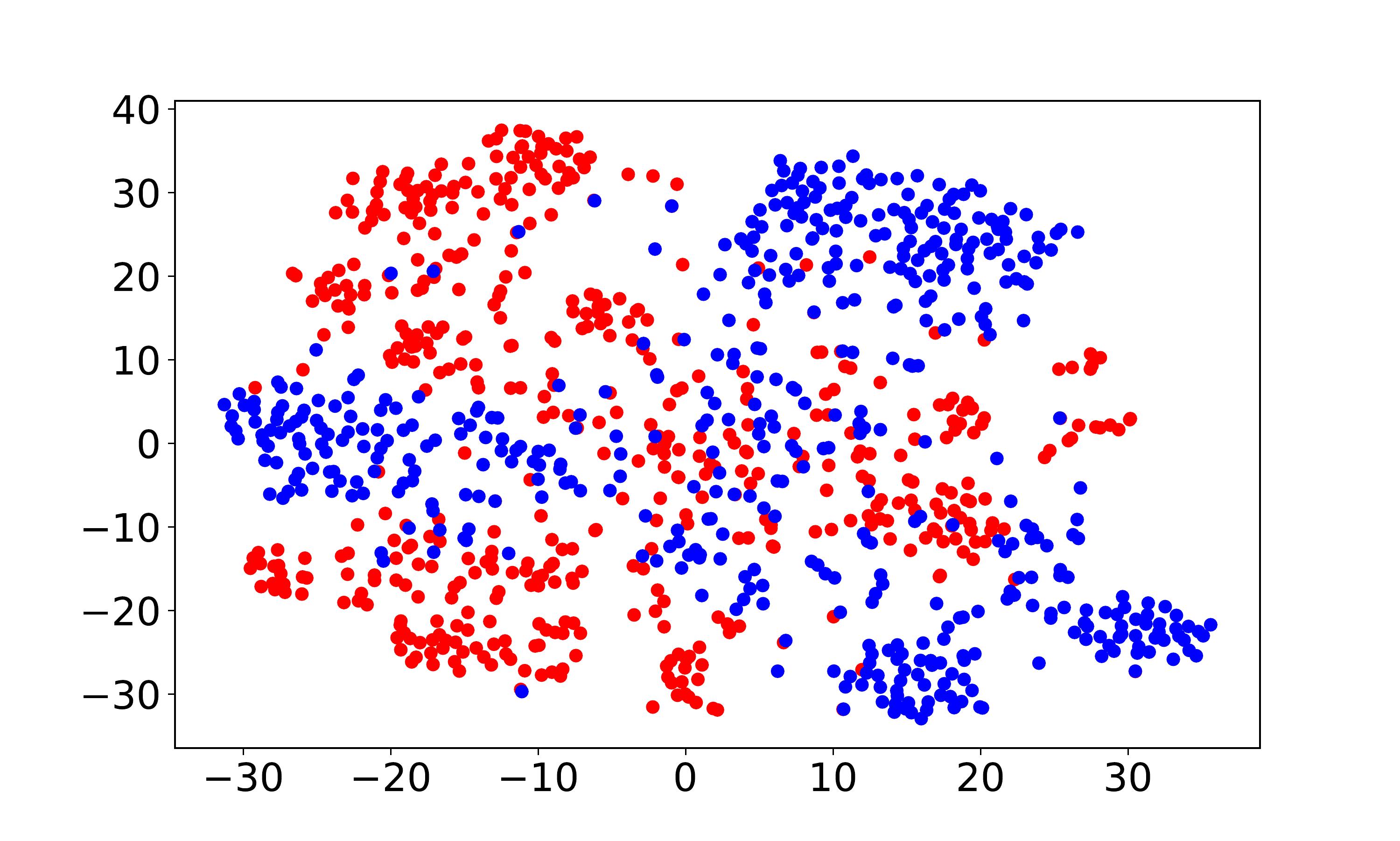
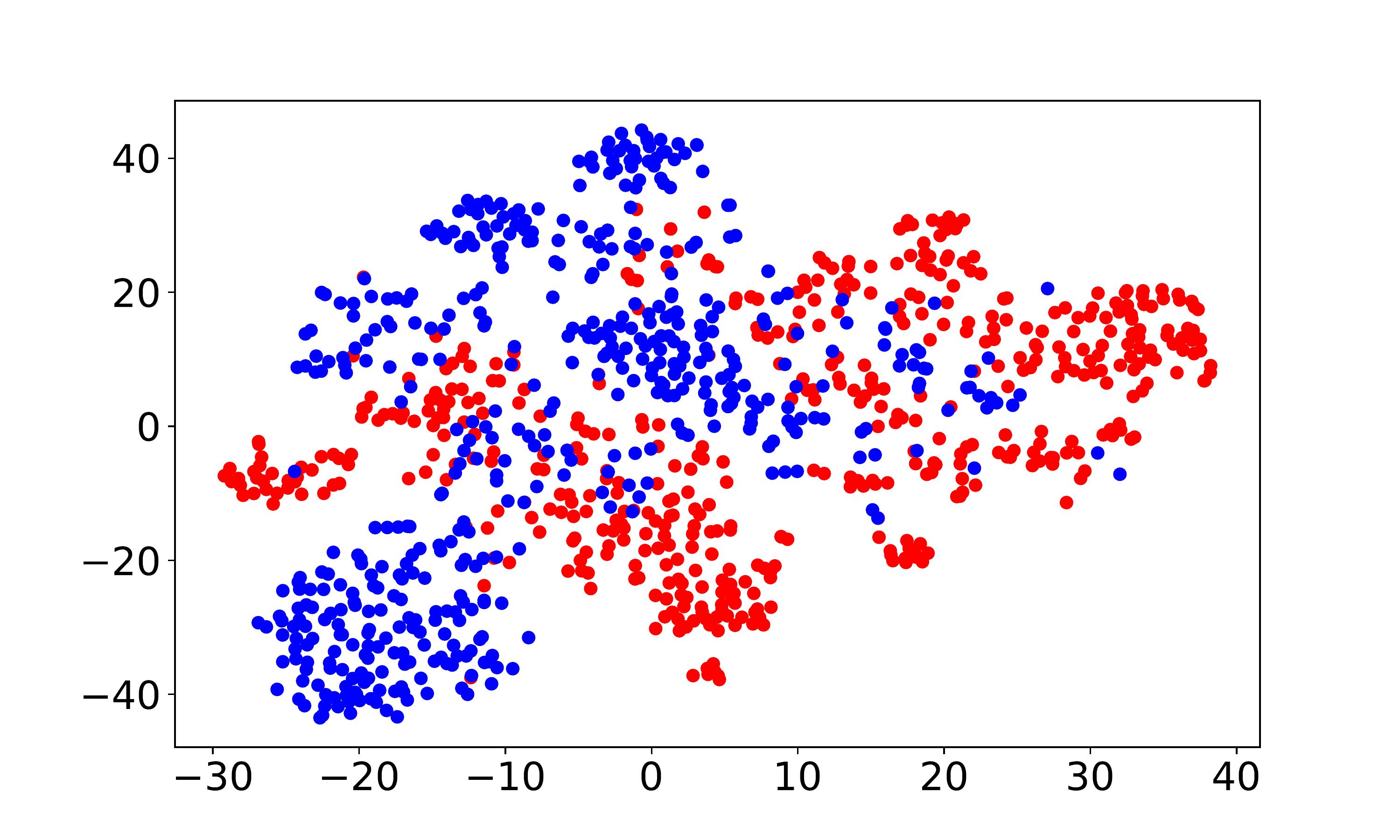
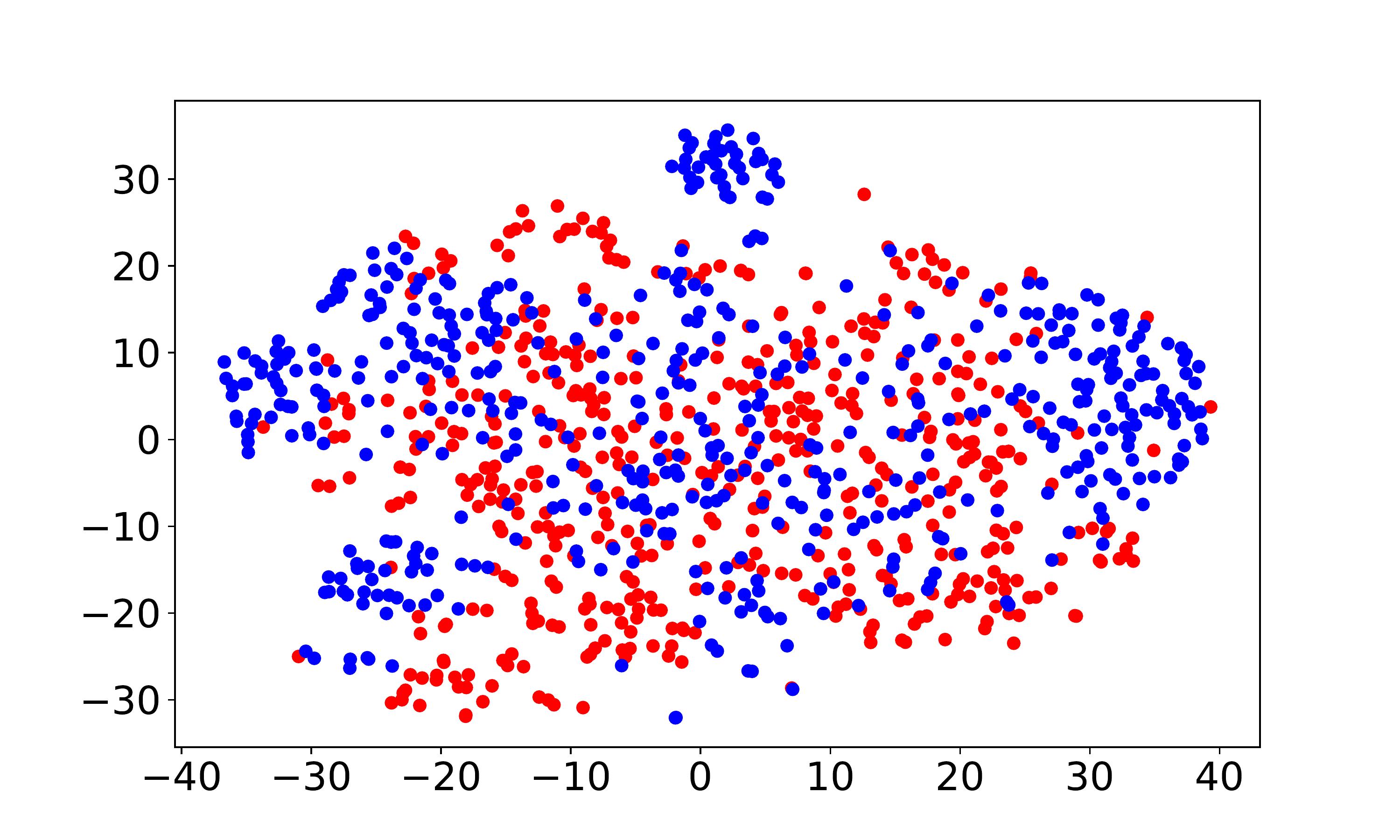
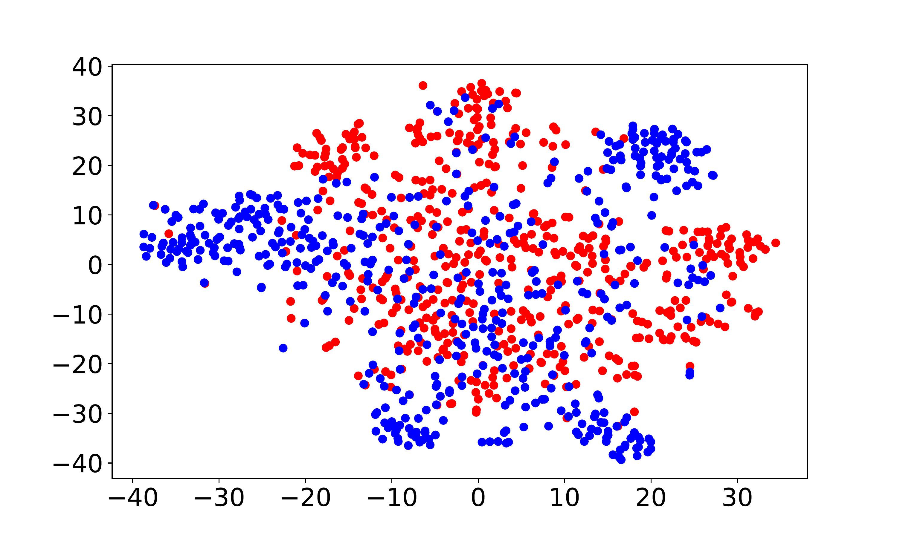
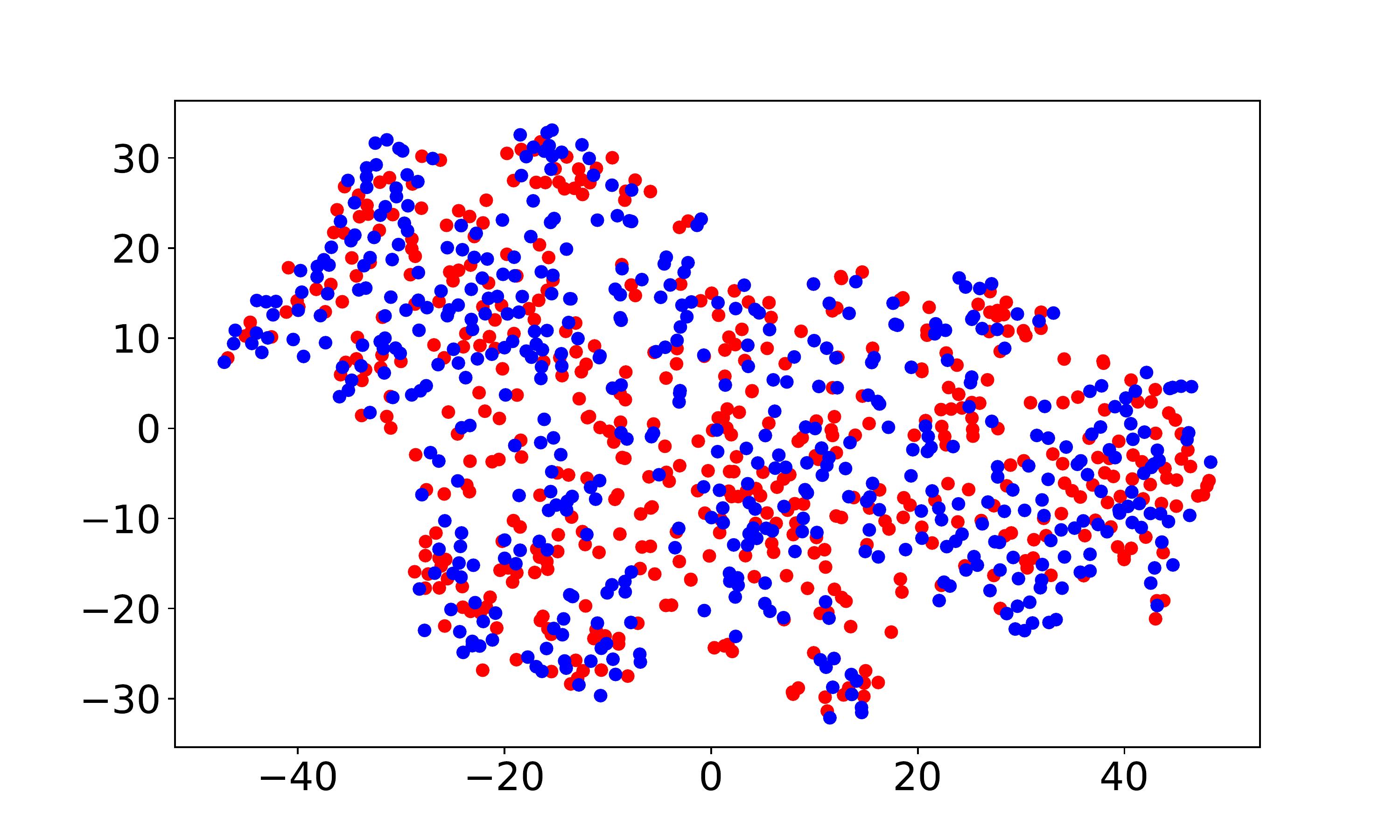
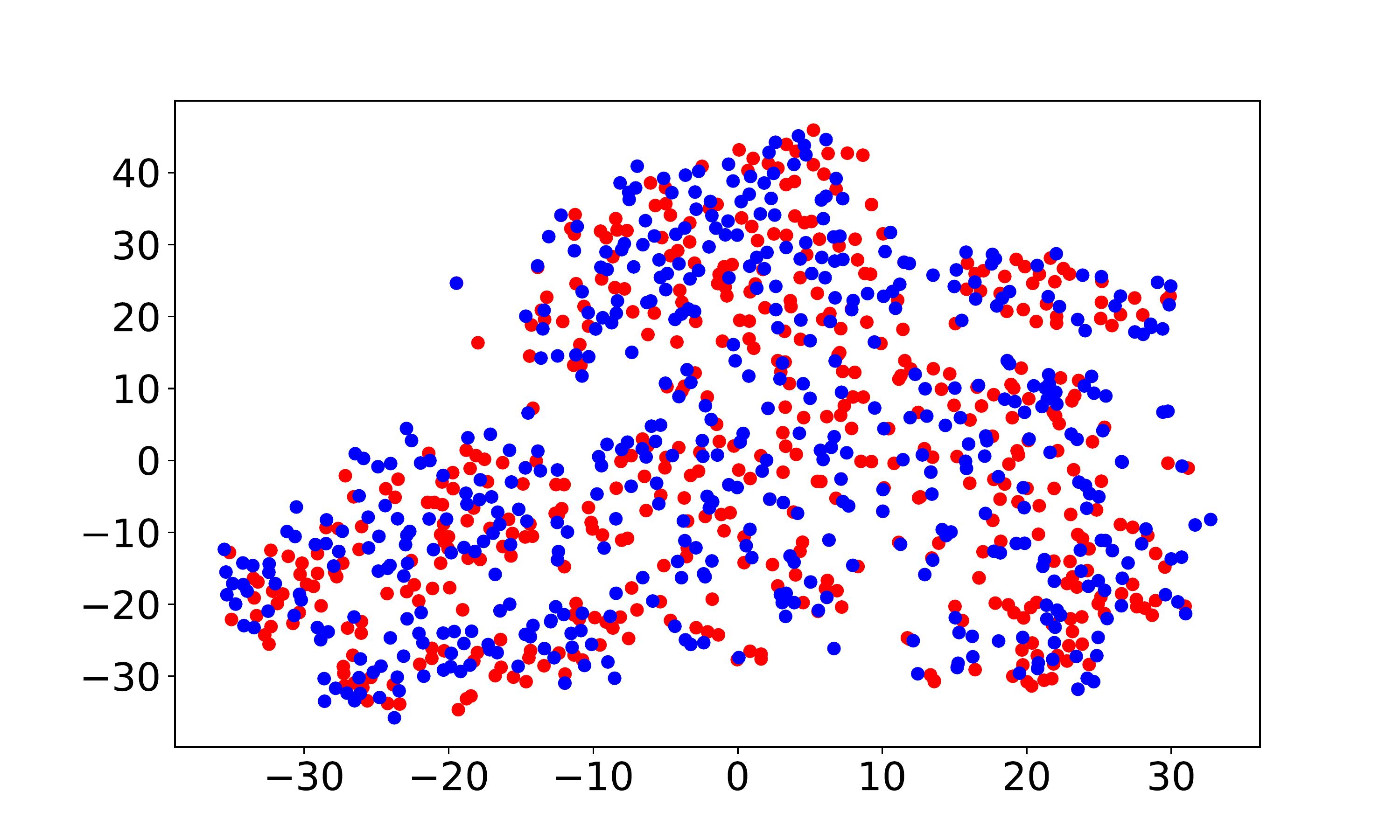
Visualization and discrepancy measurement. To better show the user embeddings across domains, we visualize the t-SNE embeddings (Laurens and Hinton, 2008) for VDEA-Base, VDEA-Local, and VDEA. The results of Amazon Movie & Book are shown in the first row of Fig. 5(a)-(c) and the results of Douban Movie & Book are shown in the second row of Fig. 5(a)-(c). From it, we can see that (1) VDEA-Base cannot bridge the user gap across different domains, leading to insufficient knowledge transfer, as shown in Fig. 5(a). (2) VDEA-Local can align some overlapped users across domains while it cannot fully minimize the global user preference discrepancy, as shown in Fig. 5(b). (3) VDEA with local and global embedding distribution alignment can better match and cluster the source and target users with similar characteristics, as shown in Fig. 5(c). The visualization result is consistent with Fig. 4(a)-(c), which illustrates the validity of our model. Moreover, we adopt to analysis the distance between two domains, where is the generalization error of a linear classifier which discriminates the source domain and the target domain (Ben-David et al., 2007). Table 4 demonstrates the domain discrepancy on Amazon Movie Amazon Book and Douban Movie Douban Book tasks using VDEA and several baseline methods. From it, we can conclude that adopting both local and global alignment in VDEA can better reduce the domain discrepancy between the source and target domains.
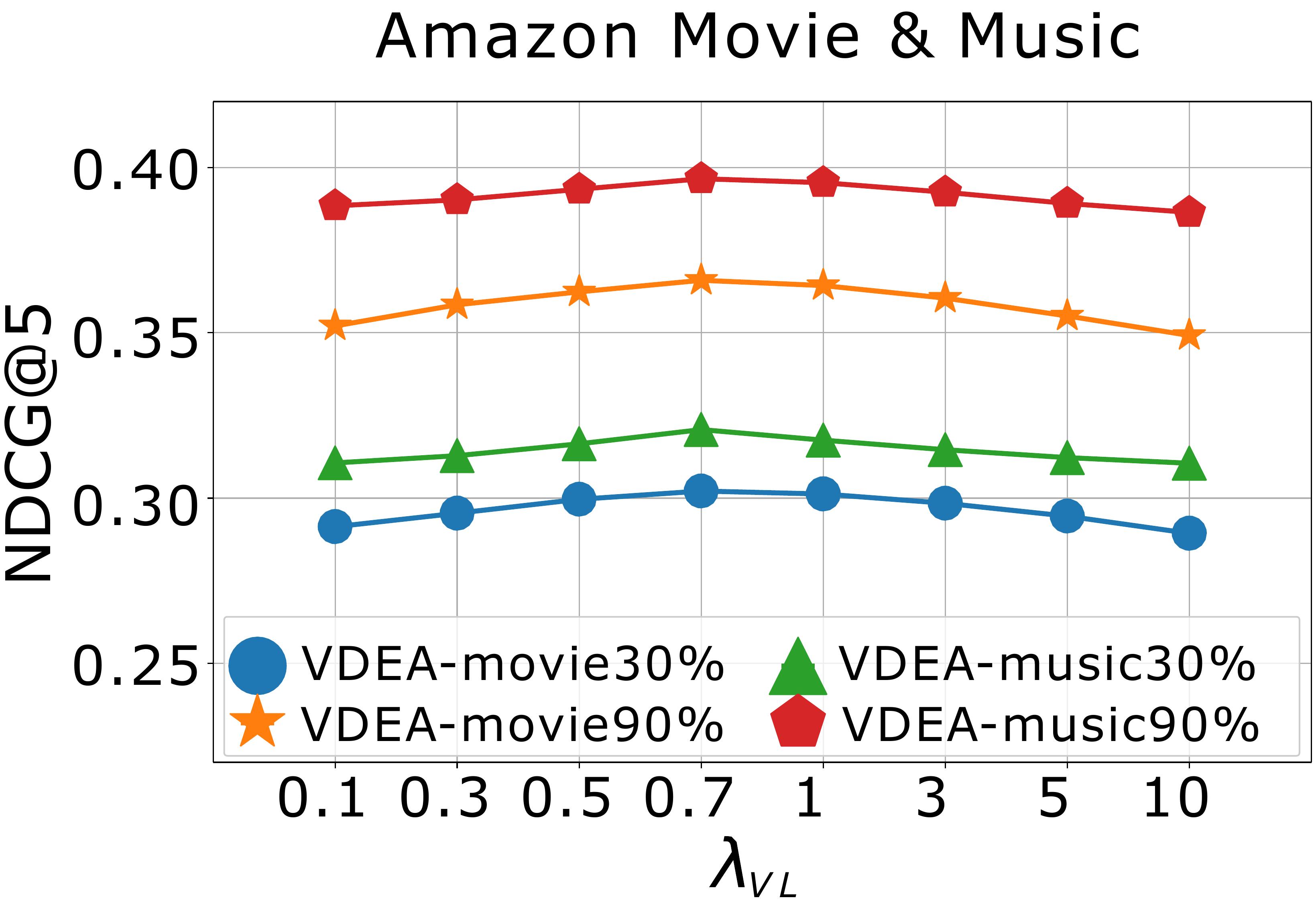
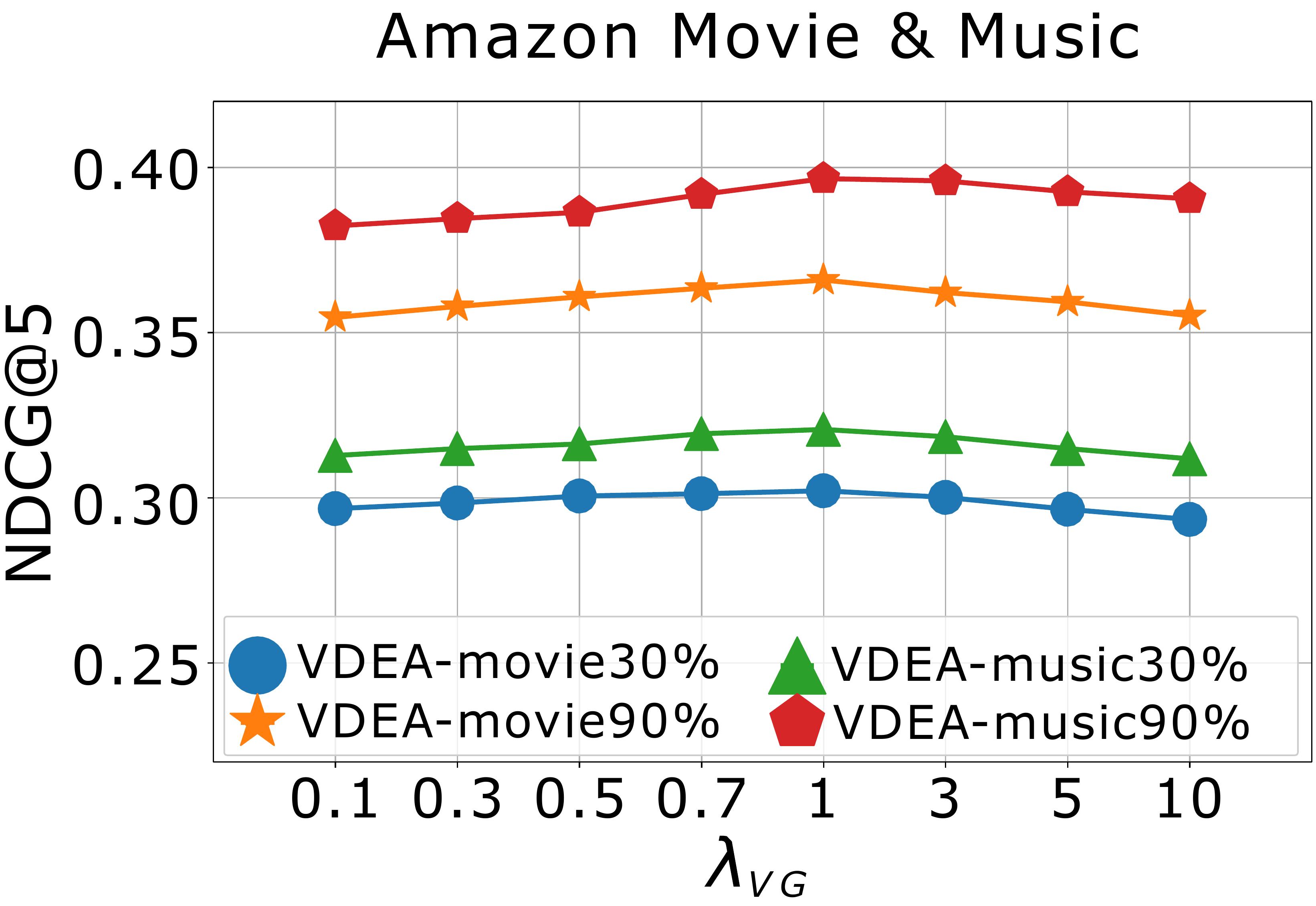
Effect of hyper-parameters. We finally study the effects of hyper-parameters on model performance, including , , , and . We first conduct experiments to study the effects of and by varying them in and report the results in Fig. 6(a)-(b). When , the alignment loss cannot produce the positive effect. When and become too large, the alignment loss will suppress the rating reconstruction loss, which also decreases the recommendation results. Empirically, we choose and . We then analyse the effect of the cluster number by varying on Amazon Music & Movie (), and report the result in Fig. 6(c). We can conclude that more clusters will enhance the model performance but it will naturally consume more time and space as well. In order to balance the model performance and operation efficiency, we recommend setting in practice. In order to investigate how the latent user embedding dimension affect the model performance, we finally perform experiment by varying dimension on VDEA. The result on Amazon Music & Movie () is shown in Fig. 6(d), where we range in . From it, we can see that, the recommendation accuracy of VDEA increases with , which indicates that a larger embedding dimension can provide more accurate latent embeddings for both users and items.
| (Amazon) Movie Book | (Douban) Movie Book | |
| DARec | 1.5032 | 1.5694 |
| DML | 1.4224 | 1.4763 |
| VDEA-Base | 1.6510 | 1.6887 |
| VDEA-Local | 1.3029 | 1.3516 |
| VDEA-Global | 1.2115 | 1.2625 |
| VDEA | 1.1644 | 1.2258 |
5. Conclusion
In this paper, we first propose Variational Dual autoencoder with Domain-invariant Embedding Alignment (VDEA), which includes the variational rating reconstruction module and the variational embedding alignment module, for solving the Partially Overlapped Cross-Domain Recommendation (POCDR) problem. We innovatively propose local and global embedding alignment for matching the overlapped and non-overlapped users across domains. We further present Mixture-Of-Gaussian distribution with Gromov-Wasserstein Distribution Co-clustering Optimal Transport (GDOT) to group the users with similar behaviors or preferences. We also conduct extensive experiments to demonstrate the superior performance of our proposed VDEA models. In the future, we plan to extend VDEA to item-based POCDR tasks and conduct more comprehensive experiments on new datasets. We are also interested in taking side-information into consideration to better solve the POCDR problem.
Acknowledgements.
This work was supported in part by the National Natural Science Foundation of China (No.72192823 and No.62172362) and Leading Expert of “Ten Thousands Talent Program” of Zhejiang Province (No.2021R52001).References
- (1)
- Angenent et al. (2003) Sigurd Angenent, Steven Haker, and Allen Tannenbaum. 2003. Minimizing flows for the Monge–Kantorovich problem. SIAM journal on mathematical analysis 35, 1 (2003), 61–97.
- Ben-David et al. (2007) Shai Ben-David, John Blitzer, Koby Crammer, and Fernando Pereira. 2007. Analysis of representations for domain adaptation. In Advances in neural information processing systems. 137–144.
- Borgwardt et al. (2006) Karsten M Borgwardt, Arthur Gretton, Malte J Rasch, Hans-Peter Kriegel, Bernhard Schölkopf, and Alex J Smola. 2006. Integrating structured biological data by kernel maximum mean discrepancy. Bioinformatics 22, 14 (2006), e49–e57.
- Chen et al. (2020b) Xu Chen, Ya Zhang, Ivor Tsang, Yuangang Pan, and Jingchao Su. 2020b. Towards Equivalent Transformation of User Preferences in Cross Domain Recommendation. arXiv preprint arXiv:2009.06884 (2020).
- Chen et al. (2020a) Zhihong Chen, Rong Xiao, Chenliang Li, Gangfeng Ye, Haochuan Sun, and Hongbo Deng. 2020a. Esam: Discriminative domain adaptation with non-displayed items to improve long-tail performance. In SIGIR. 579–588.
- Cuturi (2013) Marco Cuturi. 2013. Sinkhorn distances: Lightspeed computation of optimal transport. Advances in neural information processing systems 26 (2013), 2292–2300.
- Dacrema et al. ([n. d.]) Maurizio Ferrari Dacrema, Iván Cantador, Ignacio Fernández-Tobıas, Shlomo Berkovsky, and Paolo Cremonesi. [n. d.]. Design and Evaluation of Cross-domain Recommender Systems. ([n. d.]).
- Farseev et al. (2017) Aleksandr Farseev, Ivan Samborskii, Andrey Filchenkov, and Tat-Seng Chua. 2017. Cross-domain recommendation via clustering on multi-layer graphs. In Proceedings of the 40th International ACM SIGIR Conference on Research and Development in Information Retrieval. 195–204.
- Ganin et al. (2016) Yaroslav Ganin, Evgeniya Ustinova, Hana Ajakan, Pascal Germain, Hugo Larochelle, François Laviolette, Mario Marchand, and Victor Lempitsky. 2016. Domain-adversarial training of neural networks. The journal of machine learning research 17, 1 (2016), 2096–2030.
- He et al. (2017) Xiangnan He, Lizi Liao, Hanwang Zhang, Liqiang Nie, Xia Hu, and Tat-Seng Chua. 2017. Neural collaborative filtering. In Proceedings of the 26th international conference on world wide web. 173–182.
- Higgins et al. (2016) Irina Higgins, Loic Matthey, Arka Pal, Christopher Burgess, Xavier Glorot, Matthew Botvinick, Shakir Mohamed, and Alexander Lerchner. 2016. beta-vae: Learning basic visual concepts with a constrained variational framework. (2016).
- Hu et al. (2018) Guangneng Hu, Yu Zhang, and Qiang Yang. 2018. Conet: Collaborative cross networks for cross-domain recommendation. In Proceedings of the 27th ACM international conference on information and knowledge management. 667–676.
- Huang et al. (2018) Xun Huang, Ming-Yu Liu, Serge Belongie, and Jan Kautz. 2018. Multimodal unsupervised image-to-image translation. In ECCV. 172–189.
- Jiang et al. (2016) Zhuxi Jiang, Yin Zheng, Huachun Tan, Bangsheng Tang, and Hanning Zhou. 2016. Variational deep embedding: An unsupervised and generative approach to clustering. arXiv preprint arXiv:1611.05148 (2016).
- Kingma and Ba (2014) D. Kingma and J. Ba. 2014. Adam: A Method for Stochastic Optimization. Computer Science (2014).
- Krafft and Schmitz (1969) O Krafft and N Schmitz. 1969. A note on Hoeffding’s inequality. J. Amer. Statist. Assoc. 64, 327 (1969), 907–912.
- Laurens and Hinton (2008) Van Der Maaten Laurens and Geoffrey Hinton. 2008. Visualizing Data using t-SNE. Journal of Machine Learning Research 9, 2605 (2008), 2579–2605.
- Li et al. (2009a) B. Li, Y. Qiang, and X. Xue. 2009a. Can movies and books collaborate?: cross-domain collaborative filtering for sparsity reduction. Sun Yat-sen University 38, 4 (2009), 2052–2057.
- Li et al. (2009b) Bin Li, Qiang Yang, and Xiangyang Xue. 2009b. Transfer learning for collaborative filtering via a rating-matrix generative model. In Proceedings of the 26th annual international conference on machine learning. 617–624.
- Li and Tuzhilin (2021) Pan Li and Alexander Tuzhilin. 2021. Dual Metric Learning for Effective and Efficient Cross-Domain Recommendations. IEEE Transactions on Knowledge and Data Engineering (2021).
- Liang et al. (2018) Dawen Liang, Rahul G Krishnan, Matthew D Hoffman, and Tony Jebara. 2018. Variational autoencoders for collaborative filtering. In WWW. 689–698.
- Liu et al. (2017) Ming-Yu Liu, Thomas Breuel, and Jan Kautz. 2017. Unsupervised image-to-image translation networks. In Advances in neural information processing systems. 700–708.
- Liu et al. (2022) Weiming Liu, Xiaolin Zheng, Mengling Hu, and Chaochao Chen. 2022. Collaborative Filtering with Attribution Alignment for Review-based Non-overlapped Cross Domain Recommendation. arXiv preprint arXiv:2202.04920 (2022).
- Long et al. (2017) Mingsheng Long, Zhangjie Cao, Jianmin Wang, and Michael I Jordan. 2017. Conditional adversarial domain adaptation. arXiv preprint arXiv:1705.10667 (2017).
- Ma et al. (2019) Jianxin Ma, Chang Zhou, Peng Cui, Hongxia Yang, and Wenwu Zhu. 2019. Learning disentangled representations for recommendation. arXiv preprint arXiv:1910.14238 (2019).
- Man et al. (2017) Tong Man, Huawei Shen, Xiaolong Jin, and Xueqi Cheng. 2017. Cross-Domain Recommendation: An Embedding and Mapping Approach.. In IJCAI. 2464–2470.
- Ni et al. (2019) Jianmo Ni, Jiacheng Li, and Julian McAuley. 2019. Justifying Recommendations using Distantly-Labeled Reviews and Fine-Grained Aspects. In EMNLP-IJCNLP. 188–197. https://doi.org/10.18653/v1/D19-1018
- Pan et al. (2011) Sinno Jialin Pan, Ivor W Tsang, James T Kwok, and Qiang Yang. 2011. Domain Adaptation via Transfer Component Analysis. IEEE Transactions on Neural Networks 22, 2 (2011), 199–210.
- Santambrogio (2015) Filippo Santambrogio. 2015. Optimal transport for applied mathematicians. Birkäuser, NY 55 (2015), 58–63.
- Shenbin et al. (2020) Ilya Shenbin, Anton Alekseev, Elena Tutubalina, Valentin Malykh, and Sergey I Nikolenko. 2020. RecVAE: A new variational autoencoder for Top-N recommendations with implicit feedback. In WSDM. 528–536.
- Shu et al. (2018) Rui Shu, Hung H Bui, Hirokazu Narui, and Stefano Ermon. 2018. A dirt-t approach to unsupervised domain adaptation. arXiv preprint arXiv:1802.08735 (2018).
- Tan et al. (2018) Chuanqi Tan, Fuchun Sun, Tao Kong, Wenchang Zhang, Chao Yang, and Chunfang Liu. 2018. A survey on deep transfer learning. In International conference on artificial neural networks. Springer, 270–279.
- Tan et al. (2022) Yanchao Tan, Carl Yang, Xiangyu Wei, Chaochao Chen, Longfei Li, and Xiaolin Zheng. 2022. Enhancing Recommendation with Automated Tag Taxonomy Construction in Hyperbolic Space. (2022).
- Tan et al. (2021) Yanchao Tan, Carl Yang, Xiangyu Wei, Yun Ma, and Xiaolin Zheng. 2021. Multi-Facet Recommender Networks with Spherical Optimization. In 2021 IEEE 37th International Conference on Data Engineering (ICDE). IEEE, 1524–1535.
- Truong et al. (2021) Quoc-Tuan Truong, Aghiles Salah, and Hady W Lauw. 2021. Bilateral Variational Autoencoder for Collaborative Filtering. In Proceedings of the 14th ACM International Conference on Web Search and Data Mining. 292–300.
- Tzeng et al. (2017) Eric Tzeng, Judy Hoffman, Kate Saenko, and Trevor Darrell. 2017. Adversarial discriminative domain adaptation. In CVPR. 7167–7176.
- Villani (2008) Cédric Villani. 2008. Optimal transport: old and new. Vol. 338. Springer Science & Business Media.
- Wang et al. (2019c) Xiang Wang, Xiangnan He, Yixin Cao, Meng Liu, and Tat-Seng Chua. 2019c. Kgat: Knowledge graph attention network for recommendation. In Proceedings of the 25th ACM SIGKDD International Conference on Knowledge Discovery & Data Mining. 950–958.
- Wang et al. (2019a) Yaqing Wang, Chunyan Feng, Caili Guo, Yunfei Chu, and Jenq-Neng Hwang. 2019a. Solving the sparsity problem in recommendations via cross-domain item embedding based on co-clustering. In Proceedings of the Twelfth ACM International Conference on Web Search and Data Mining. 717–725.
- Wang et al. (2019b) Yaqing Wang, Chunyan Feng, Caili Guo, Yunfei Chu, and Jenq-Neng Hwang. 2019b. Solving the sparsity problem in recommendations via cross-domain item embedding based on co-clustering. In Proceedings of the Twelfth ACM International Conference on Web Search and Data Mining. 717–725.
- Weike et al. (2013) Weike, Pan, , , Qiang, and Yang. 2013. Transfer learning in heterogeneous collaborative filtering domains. Artificial Intelligence (2013).
- Xu et al. (2020) Hongteng Xu, Dixin Luo, Ricardo Henao, Svati Shah, and Lawrence Carin. 2020. Learning autoencoders with relational regularization. In International Conference on Machine Learning. PMLR, 10576–10586.
- Yu et al. (2020) Wenhui Yu, Xiao Lin, Junfeng Ge, Wenwu Ou, and Zheng Qin. 2020. Semi-supervised collaborative filtering by text-enhanced domain adaptation. In Proceedings of the 26th ACM SIGKDD International Conference on Knowledge Discovery & Data Mining. 2136–2144.
- Yuan et al. (2019) Feng Yuan, Lina Yao, and Boualem Benatallah. 2019. DARec: Deep domain adaptation for cross-domain recommendation via transferring rating patterns. arXiv preprint arXiv:1905.10760 (2019).
- Zhang et al. (2018) Qian Zhang, Jie Lu, Dianshuang Wu, and Guangquan Zhang. 2018. A cross-domain recommender system with kernel-induced knowledge transfer for overlapping entities. IEEE transactions on neural networks and learning systems 30, 7 (2018), 1998–2012.
- Zhao et al. (2020) Cheng Zhao, Chenliang Li, Rong Xiao, Hongbo Deng, and Aixin Sun. 2020. CATN: Cross-Domain Recommendation for Cold-Start Users via Aspect Transfer Network. 229–238. https://doi.org/10.1145/3397271.3401169
- Zhu et al. (2019) Feng Zhu, Chaochao Chen, Yan Wang, Guanfeng Liu, and Xiaolin Zheng. 2019. DTCDR: A framework for dual-target cross-domain recommendation. In CIKM. 1533–1542.
- Zhu et al. (2021a) Feng Zhu, Yan Wang, Chaochao Chen, Jun Zhou, Longfei Li, and Guanfeng Liu. 2021a. Cross-Domain Recommendation: Challenges, Progress, and Prospects. arXiv preprint arXiv:2103.01696 (2021).
- Zhu et al. (2021b) Feng Zhu, Yan Wang, Jun Zhou, Chaochao Chen, Longfei Li, and Guanfeng Liu. 2021b. A unified framework for cross-domain and cross-system recommendations. IEEE Transactions on Knowledge and Data Engineering (2021).
- Zhuang et al. (2021) Fuzhen Zhuang, Zhiyuan Qi, Keyu Duan, Dongbo Xi, Yongchun Zhu, Hengshu Zhu, Hui Xiong, and Qing He. 2021. A Comprehensive Survey on Transfer Learning. Proc. IEEE 109, 1 (2021), 43–76. https://doi.org/10.1109/JPROC.2020.3004555