Exploring The Effect of High-frequency Components in GANs Training
Abstract
Generative Adversarial Networks (GANs) have the ability to generate images that are visually indistinguishable from real images. However, recent studies have revealed that generated and real images share significant differences in the frequency domain. In this paper, we explore the effect of high-frequency components in GANs training. According to our observation, during the training of most GANs, severe high-frequency differences make the discriminator focus on high-frequency components excessively, which hinders the generator from fitting the low-frequency components that are important for learning images’ content. Then, we propose two simple yet effective frequency operations for eliminating the side effects caused by high-frequency differences in GANs training: High-Frequency Confusion (HFC) and High-Frequency Filter (HFF). The proposed operations are general and can be applied to most existing GANs with a fraction of the cost. The advanced performance of the proposed operations is verified on multiple loss functions, network architectures, and datasets. Specifically, the proposed HFF achieves significant improvements of FID on CelebA (128*128) unconditional generation based on SNGAN, FID on CelebA unconditional generation based on SSGAN, and FID on CelebA unconditional generation based on InfoMAXGAN.
I Introduction
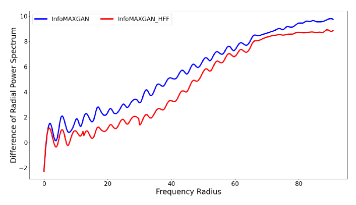
Generative Adversarial Networks (GANs) [1] have been widely used in the field of computer vision and image processing: attribute editing [2, 3], generation of photo-realistic images [4, 5], image inpainting [6, 7]. Although the remarkable advancements in community, recent works [8, 9, 10, 11, 12, 13] have demonstrated that generated images are significantly different from real images in the frequency domain, especially in the high frequency. As shown in Figure 1(a), the frequency bias between real and generated images increases with the frequency. There are two main hypotheses for the artifacts with generated images in the frequency domain: some studies [13, 10, 12] suggest that this difference is mainly due to the employed of upsampling operations; and some studies [8, 9] suggest that the linear dependencies in the Conv filter’s spectrum cause spectral limitations.
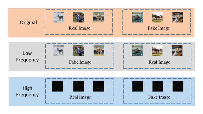
GANs training is a dynamic game. A good discriminator is a prerequisite for training the generator. Existing discriminators directly use all information of the generated and real images to make the ‘true/fake’ decision, which could introduce some shortcut during GANs training. Figure 1(b) illustrates several examples of predicting defect of the discriminator in the frequency domain, which indicates that the discriminator is sensitive to the high-frequency components and relies on the high-frequency information as the shortcut to make their decision. In this study, we comprehensively explore and analyze the impact of high-frequency components during the training of GANs.
High-frequency components of images contain limited information [15] and are difficult to be fitted [8]. Too much focus on high-frequency biases degrades the fit of generator to low-frequency components because the generator may be optimized to fool the discriminators by perturbing high-frequency components. Based on this, we propose two frequency operations (HFC and HFF) for removing the high-frequency biases during the training of GANs, which alleviates the sensitivity of the discriminator to high-frequency biases and focuses more on low-frequency components. Among them, High-Frequency Confusion (HFC) replaces the high-frequency components of the generated images with the high-frequency components of real images, while High-Frequency Filter (HFF) filters out the high-frequency components of both real and generated images. Figure 1(a) shows the frequency bias between real and fake images generated by InfoMAXGAN and InfoMAXGAN with HFF. The result demonstrates that the proposed method can effectively mitigate the low-frequency bias without compromising the high-frequency fit. Although frequency biases, especially at high frequencies, are not completely eliminated, the proposed methods are general and can be applied to most existing GANs frameworks with a fraction of the cost. We also hope this paper can inspire more works in this area to better solve the frequency bias problem.
The main contributions of this paper can be summarized as follows:
-
•
This paper aims for the first pilot study to analyze the frequency response in GANs. According to experiments analysis, we demonstrate that discriminator is sensitive to the high-frequency components of images and the high-frequency biases between real and fake images affect the fit of low-frequency components during the training of generators.
-
•
To balance the high-frequency biases between the generated and the real images during the training of GANs, two simple yet effective frequency operations are proposed in this paper. We confirm that the proposed methods can improve the fit of generator to the low-frequency components effectively.
-
•
Comprehensive experiments valid the superiority of our proposed operations. Besides low-frequency components, the proposed operations improve the quality of overall generation on many loss functions, architectures, and datasets with little cost.
II Related Works
II-A Generative Adversarial Networks
Generative Adversarial Networks (GANs) act a two-player adversarial game, where the generator is a distribution mapping function that transforms low-dimensional latent distribution to target distribution . And the discriminator evaluates the distance between generated distribution and real distribution . The generator and discriminator minimize and maximize the zero-sum loss function, respectively. This minimax game can be expressed as:
| (1) |
where and are parameters of the generator and discriminator , respectively. Specifically, vanilla GAN [1] can be described as ; -GAN [16] can be written as ; Morever, Geometric GAN [17] and WGAN [18] are described as and , respectively.
Recently, the quality of the generated images has been improved dramatically. Karras et al. [19] describe a new training methodology in GANs, which grows both the generator and discriminator progressively. The progressive training method makes the quality of high-resolution image synthesis improved unprecedentedly. Also, Karras et al. propose StyleGAN [4] and StyleGAN++ [5], which use style-based method to the generation of specific content. Furthermore, some regularization and normalization methods are used to stabilize GANs training [20], WGAN-GP [21] and SNGAN [14] apply 1-Lipschitz continuity using gradient penalty and spectral normalization, respectively; GAN-DAT [22] minimizes Lipschitz constant to avoid the discriminator being attacked by the adversarial examples; SS-GAN [23] uses self-supervised techniques to avoid discriminator forgetting; Similarly, InfoMAXGAN [24] improves the image generation via information maximization and contrastive learning, which is an unsupervised method for mitigating catastrophic forgetting.
In this paper, two frequency operations are used in three loss functions: vanilla GAN loss, LSGAN loss, Geometric loss (Hinge loss) and three frameworks: SNGAN, SSGAN, and InfoMAXGAN. Experiments demonstrate the consistent improvement of our methods.
II-B Frequency Principle for CNNs
Recently, frequency analysis on Convolution Neural Networks (CNNs) has attracted more and more attention. According to the different analysis objects, related studies can be divided into two categories: Input (Image) Frequency and Response Frequency. Many works have shown that there is a principle in both categories of frequency: DNNs often fit target functions from low to high frequencies during the training, which is called Frequency Principle (F-Principle) in [25, 26] or Spectral Bias in [27]. Input (Image) Frequency corresponds to the rate of change of intensity across neighboring pixels of input images, where sharp textures contribute to the high frequency of the image. Wang et al. [15] demonstrate the F-Principle of Input Frequency and point that the high-frequency components of the image improve the performance of the model, but reduce its generalization.
Furthermore, Response Frequency is the frequency of general Input-Output mapping , which measures the rate of change of outputs with respect to inputs. If possesses significant high frequencies, then a small change of inputs in the image might induce a large change of the output (e.g. adversarial example in [28]). F-Principle of Response Frequency is first proposed by Xu et al. [25] through regression problems on synthetic data and real data with principal component analysis. Similarly, Rahaman et al. [27] find empirical evidence of a spectral bias: lower frequencies are learned first. They also show that lower frequencies are more robust to random perturbations of the network parameters. Subsequently, Xu et al. [29] propose a theoretical analysis framework for one hidden layer neural network with 1-d input, which illustrates activation functions (including Tanh and Relu) in the Fourier domain decays as frequency increases. Furthermore, Xu et al. [26] also propose a Gaussian filtering method that can directly verify the F-Principle in high-dimensional datasets for both regression and classification problems. Certainly, there are still a lot of works [30, 31, 32, 33, 34] to be done in the frequency domain to interpret the success and failure of CNNs.
II-C Frequency Bias for GANs
Frequency analysis of GANs is also popular, from which we are mainly concerned with the Input (Image) Frequency. The frequency bias of GANs mainly refers to the bias between the generated images and the real images in the frequency domain, which can be observed in Figure 1(a). The same phenomenon has also been found in other works [13, 12, 9, 11, 10, 8]. All of them demonstrate that this phenomenon is pervasive and hard to avoid, even if some generated images are flawless from human perception. In addition to two main hypotheses (i.e. the employment of upsampling operations and linear dependencies in the Conv filter’s spectrum) introduced in the Introduction, Chen et al. [11] reveal that downsampling layers cause the high frequencies missing in the discriminator. This issue may make the generator lacking the gradient information to model high-frequency content, resulting in a significant spectrum discrepancy between generated images and real images. To solve it, they propose the SSD-GAN that boosts a frequency-aware classifier into the discriminator to measure the realness of images in both spatial and spectral domains.
Although the proposed SSD-GAN [11] improves the performance of GANs by increasing the discrimination of discriminator in spectral domain, our proposed HFF and HFC are orthogonal to it and the performance of SSD-GAN can also be further improved. The study that most closely resembles our paper is proposed by Yamaguchi et al. [35]. Both methods have filtered out unnecessary high-frequency components of the images during the discriminator training. In addition, our method111The Preprint of our work was published to arXiv (https://arxiv.org/abs/2103.11093) on March 20, 2021. However, the Preprint of [35] was published to arXiv (https://arxiv.org/pdf/2106.02343) on June 4, 2021. analyze the response of discriminator to different-frequency components.
III Methodology
In this section, we first demonstrate frequency decomposition and mixing of images. Then we analyze the discriminator’s response for different frequency components. Based on these, we propose two frequency operations to reduce the focus on high-frequency bias between real and fake images during the training of GANs, thereby enhancing the fit of low-frequency components.
III-A Frequency Decomposition and Mixing of Images
For decomposing and mixing different components of images in frequency domain, we first show the DFT of 2D image data with size :
| (2) |
And the Power Spectrum (PS) of DFT is defineds as . At the last, the Radial Power Spectrum (RPS) of DFT via azimuthal integration can be shown as:
| (3) |
where is the radius of the frequency. Figure 1(a) illustrates the RPS of real and fake images on the CelebA dataset.
In adition, we also introduce a threshold function that separates the low and high frequency components according to the radius . The formal definition of the equation is as follows:
| (4) |
where represents the value of at position index and indicate the index of the center point of the image. We use as the Euclidean distance.
In this paper, frequency decomposition and frequency mixing of the real image and the generated image are defined as follows:
| (5) |
where represents the high-frequency components of another real image that is different from . represents the high-frequency components of another generated image that is different from .
The equations in Eq (LABEL:Eq:4) define the different frequency components of the image, some are frequency decompositions (, , , and ) and some are frequency mixtures (, , , and ). Properties of these frequency components will be discussed in the following sections.
III-B High Frequency Filter (HFF) and High Frequency Confusion (HFC)
In this subsection, we first analyze the response of discriminator to different frequency components and demonstrate that discriminator in GANs is sensitive to high-frequency components of the images. And then, we propose two frequency operations to eliminate the bias between the generated images and the real images during the training of GANs.
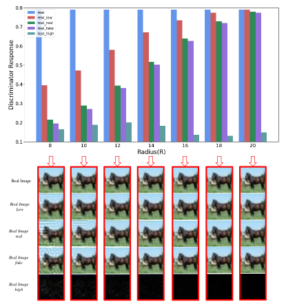
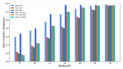
First, we analyze the responses of the discriminator to different frequency components introduced in Eq (LABEL:Eq:4). The mean values of the discriminator output on the CIFAR-10 dataset for different frequency components of real images are shown at the top part of Figure 2, where real, real_low, real_real, real_fake, and real_high represent , , , , and , respectively. Furthermore, the visualization of different frequency components in the real images is also shown at the bottom part of Figure 2. The result illustrates that the trained discriminator has differences in response to different frequency components (, , and ), even when . It is worth noting that under different threshold radius (R), (1) the output of is always lower than that of ; (2) the output of is always higher than that of , which indicates that high-frequency components of images are critical to training the discriminator, and it also demonstrates that the bias between real images and generated images at high frequency is universal.
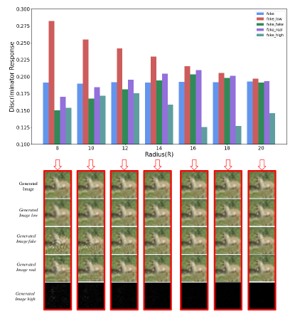
Furthermore, we demonstrate the response of the discriminator to the generated images on the CIFAR-10 dataset in Figure 3, where fake, fake_low, fake_fake, fake_real, and fake_high represent , , , , and in the Eq (4). Similar to the response of real images, the output of is lower than that of . The output of is always the highest, even higher than , no matter what is.
Second, Figure 1(b) illustrates some predicting defects of discriminator in the frequency domain. Original images and high-frequency components have the same prediction by the trained discriminator, while low-frequency components similar to the original image have a different prediction, which is not in line with human expectations. The results further demonstrate that discriminator of GANs is sensitive to high-frequency components of images.
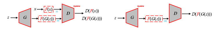
It is reasonable to believe that the discriminator in GANs is sensitive to high-frequency components that is hard to be distinguished by humans. Meanwhile, the high-frequency components of images affect the training of GANs. Based on above analyses, we propose two frequency operations to eliminate high-frequency involvement during the training of GANs, which can improve the fit of the overall distribution, especially low-frequency components. Figure 4 illustrates the overview of the HFF and HFC for updating discriminator and generator during GANs training, the loss functions are:
| (6) |
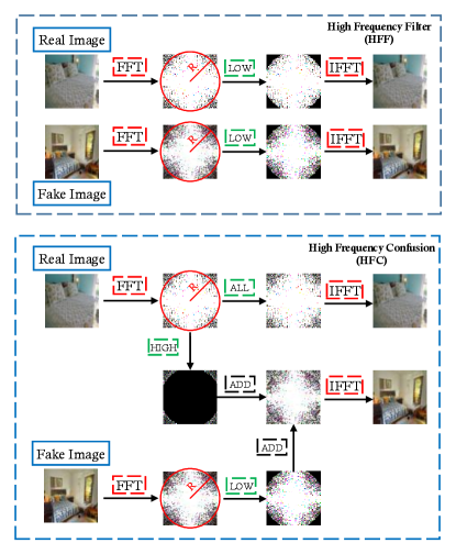
where is required to be the same function (HFF or HFC) and the same threshold radius (R) across the three places illustrated in Figure 4. The framework of HFF and HFC can be seen in Figure 5, where HFF uses a filter to filter out the high-frequency components of the images, while HFC mixes two types of images by replacing the high-frequency components of the generated images with the high-frequency components of the real images. The form can be expressed as:
| (7) |
| Method | Where ? | Radius (R) | ||||||||
| (i) | (ii) | (iii) | 12 | 14 | 16 | 18 | 20 | 22 | ||
| SNGAN(Baseline) | 20.05 | 20.05 | 20.05 | 20.05 | 20.05 | 20.05 | ||||
| SNGAN-HFF (Real only) | ✓ | 26.65 | 23.59 | 20.02 | 20.3 | 19.68 | 20.16 | |||
| SNGAN-HFF (Fake only) | ✓ | 350 | 350 | 100 | 68 | 20.07 | 20.67 | |||
| SNGAN-HFF (Dis only) | ✓ | ✓ | 350 | 52.2 | 20.07 | 20.59 | 19.89 | 19.53 | ||
| SNGAN-HFF (All) | ✓ | ✓ | ✓ | 21.29 | 21.06 | 18.74 | 18.5 | 18.54 | 19.59 | |
At the end, we also analyze the impact of the HFF for discriminator response. Figure 6 demonstrates the output of the discriminator to real images using the HFF before-and-after, respectively, where HFF indicates that the discriminator is trained with the proposed HFF method. The results illustrate: (1) the discriminator output of HFF_real_low is almost higher (i.e. more confidence) than that of real_low; (2) The gap between HFF_real_real and HFF_real_fake is less than the gap between real_real and real_fake. In particular, when the filter Radius (R) is greater than 16, the gap between HFF_real_real and HFF_real_fake is 0; (3) When the radius is greater than 8, the discriminator outputs of HFF_real_real and HFF_real_fake are also greater than that of real_real and real_fake. These three points demonstrate that the proposed HFF alleviates the sensitivity of discriminator to high-frequency and improves the fit of discriminator to the low-frequency components.
IV Experiments
In the experimental section, we evaluate the proposed methods (HFF and HFC) on GANs training of different loss functions, network architectures, and datasets. The results demonstrate that high-frequency bias affects the fit of generator, and the proposed methods improve the generative performance of GANs. The details of datasets and experiment settings are shown in Section A of the Supplementary Materials.
IV-A The Results on CIFAR-10 Dataset with Different Places
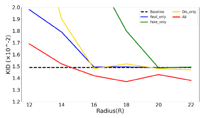
In this subsection, we apply the proposed HFF to different places ((i), (ii), (iii) in Figure 4) of the GANs training. Frechet Inception Distance (FID) and Kernel Inception Distance (KID) with using HFF in different places for training the GANs on the CIFAR-10 dataset are shown in Table I and Figure 7, respectively. The results illustrate: (1) Excessive filtering of high-frequency components makes the training of ”Real only”, ”Fake only”, and ”Dis only” methods fail, and reduces the performance of the ”All” method; (2) When the threshold radius (R) is relatively large, performance of ”Real only”, ”Fake only”, and ”Dis only” methods are similar to that of existing GANs (baseline), while performance of the ”All” method is better than that of baseline. These results show that adding artificial high-frequency bias (using ”Real only” or ”Fake only” methods only filter high-frequency components of real or fake images, which introduces the artificial high-frequency bias during the GANs training) between the real images and the generated images has little effect on the training of GANs, while removing the high-frequency bias between the generated images and the real images (”All”) improves the performance of GANs, which indicates that both natural and artificial high-frequency biases are not beneficial to the training of GANs.
IV-B The Results on CIFAR-10 Dataset with Different Loss Functions
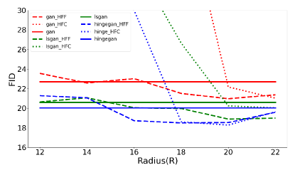
This subsection validates whether our proposed frequency opeartions are robust to different loss functions. Three different loss functions (vanilla GAN [1], LSGAN [36], hinge GAN [17]) are used to train SNGAN on the CIFAR-10 dataset. FID and Inception Score (IS) are shown in Figure 8 and Table II, respectively. Compared to HFF, it is easy to understand that HFC fails to train at small Radius. HFC replaces the high-frequency components of the generated images with the high-frequency components of the real images, which leads to a significant discontinuity in the spectrum domain of the generated images as shown in Figure 5. The spectral discontinuity of the generated images leads to deviations between them and the real images, which leads to the fail of training. When R is large, this spectral discontinuity is minor, and the deviations between real images and generated images are imperceptible. Hence HFC is only suitable for larger radius.
The proposed HFC and HFF both improve the performance of the baseline. Furthermore, the best performances of HFF and HFC are achieved when R equals to 20 (the vast majority of cases), which corresponds to the phenomenon illustrated in the upper and left part of the Figure 10 (High-frequency bias occurs at the radius of 20 on the CIFAR-10 dataset).
| Loss | Method | Radius (R) | ||||||
| 12 | 14 | 16 | 18 | 20 | 22 | (Baseline) | ||
| gan | HFF | |||||||
| HFC | ||||||||
| lsgan | HFF | |||||||
| HFC | ||||||||
| hinge gan | HFF | |||||||
| HFC | ||||||||
IV-C Evaluation on Different Datasets and Different Architectures
In this subsection, HFF and HFC are adopted on some popular models, such as SNGAN, SSGAN, and InfoMAXGAN. Hinge loss is selected for all experiments. The baseline codes are available on Github222https://github.com/kwotsin/mimicry. We evaluate our methods on five different datasets at multiple resolutions: CIFAR-10 () [37], CIFAR-100 () [37], STL-10 () [38], LSUN-Bedroom () [39], and CelebA (). Also, three metrics are adopted to evaluate the quality of generated images: Fréchet Inception Distance (FID) [40], Kernel Inception Distance (KID) [41], and Inception Score (IS) [42].
| Metric | Dataset | Models | ||||||||
| SNGAN | SSGAN | InfoMAX-GAN | ||||||||
| None | HFF | HFC | None | HFF | HFC | None | HFF | HFC | ||
| FID | CelebA | 12.46 | 7.17 | 10.43 | 8.90 | 6.21 | 7.44 | 21.52 | 6.59 | 6.25 |
| LSUN-Bedroom | 40.47 | 37.71 | 38.77 | 40.01 | 35.79 | 38.36 | 40.32 | 39.37 | 39.79 | |
| STL-10 | 40.77 | 38.99 | 38.43 | 38.78 | 35.13 | 35.14 | 38.55 | 37.44 | 38.64 | |
| CIFAR-100 | 23.70 | 21.45 | 21.98 | 22.43 | 20.27 | 21.51 | 21.36 | 20.41 | 19.16 | |
| CIFAR-10 | 20.05 | 18.54 | 18.28 | 16.75 | 14.71 | 14.88 | 17.71 | 16.19 | 17.17 | |
| KID () | CelebA | 0.91 | 0.51 | 0.67 | 0.62 | 0.42 | 0.51 | 1.65 | 0.43 | 0.43 |
| LSUN-Bedroom | 4.86 | 4.22 | 4.65 | 4.75 | 4.36 | 4.53 | 4.81 | 4.66 | 4.72 | |
| STL-10 | 3.84 | 3.68 | 3.77 | 3.62 | 3.28 | 3.31 | 3.69 | 3.54 | 3.72 | |
| CIFAR-100 | 1.58 | 1.31 | 1.35 | 1.55 | 1.4 | 1.56 | 1.52 | 1.39 | 1.33 | |
| CIFAR-10 | 1.49 | 1.38 | 1.35 | 1.25 | 1.13 | 1.13 | 1.34 | 1.12 | 1.24 | |
| IS | CelebA | - | - | - | - | - | - | - | - | - |
| LSUN-Bedroom | - | - | - | - | - | - | - | - | - | |
| STL-10 | 8.43 | 8.58 | 8.54 | 8.58 | 8.79 | 8.76 | 8.63 | 8.74 | 8.69 | |
| CIFAR-100 | 7.66 | 7.85 | 7.84 | 7.74 | 7.85 | 7.96 | 8.02 | 8.02 | 8.1 | |
| CIFAR-10 | 7.84 | 7.95 | 8.01 | 8.13 | 8.1 | 8.09 | 8.01 | 8.1 | 8.0 | |
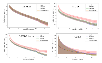
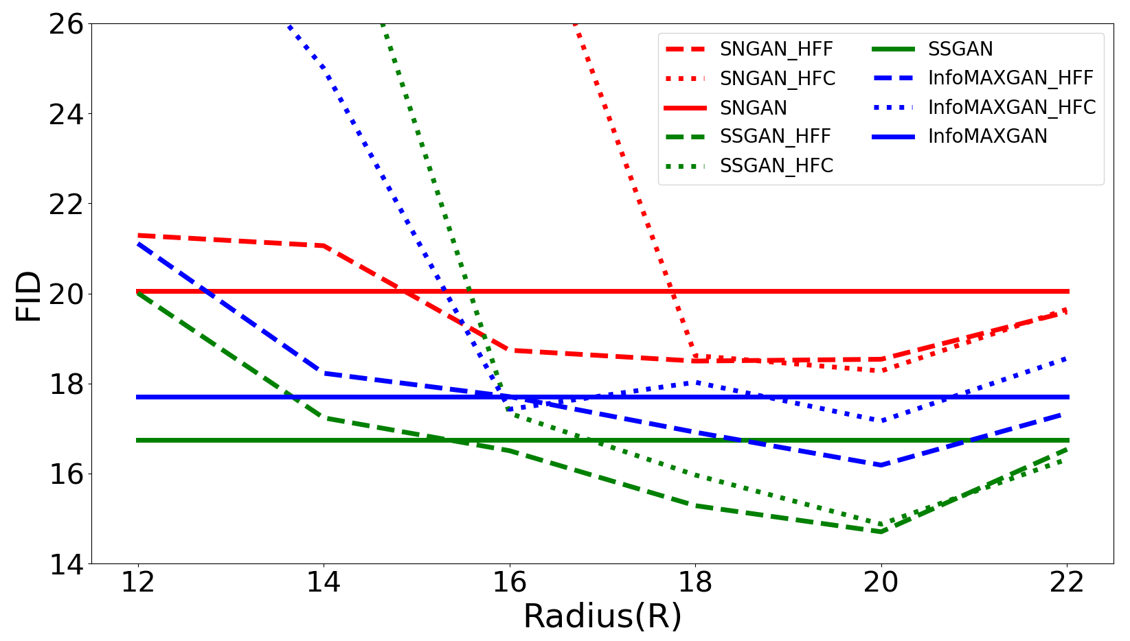
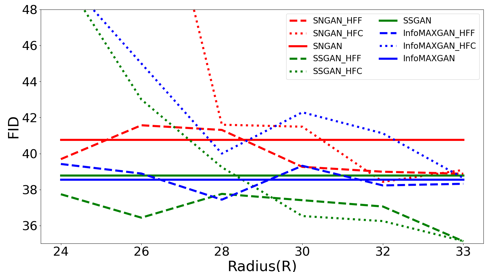
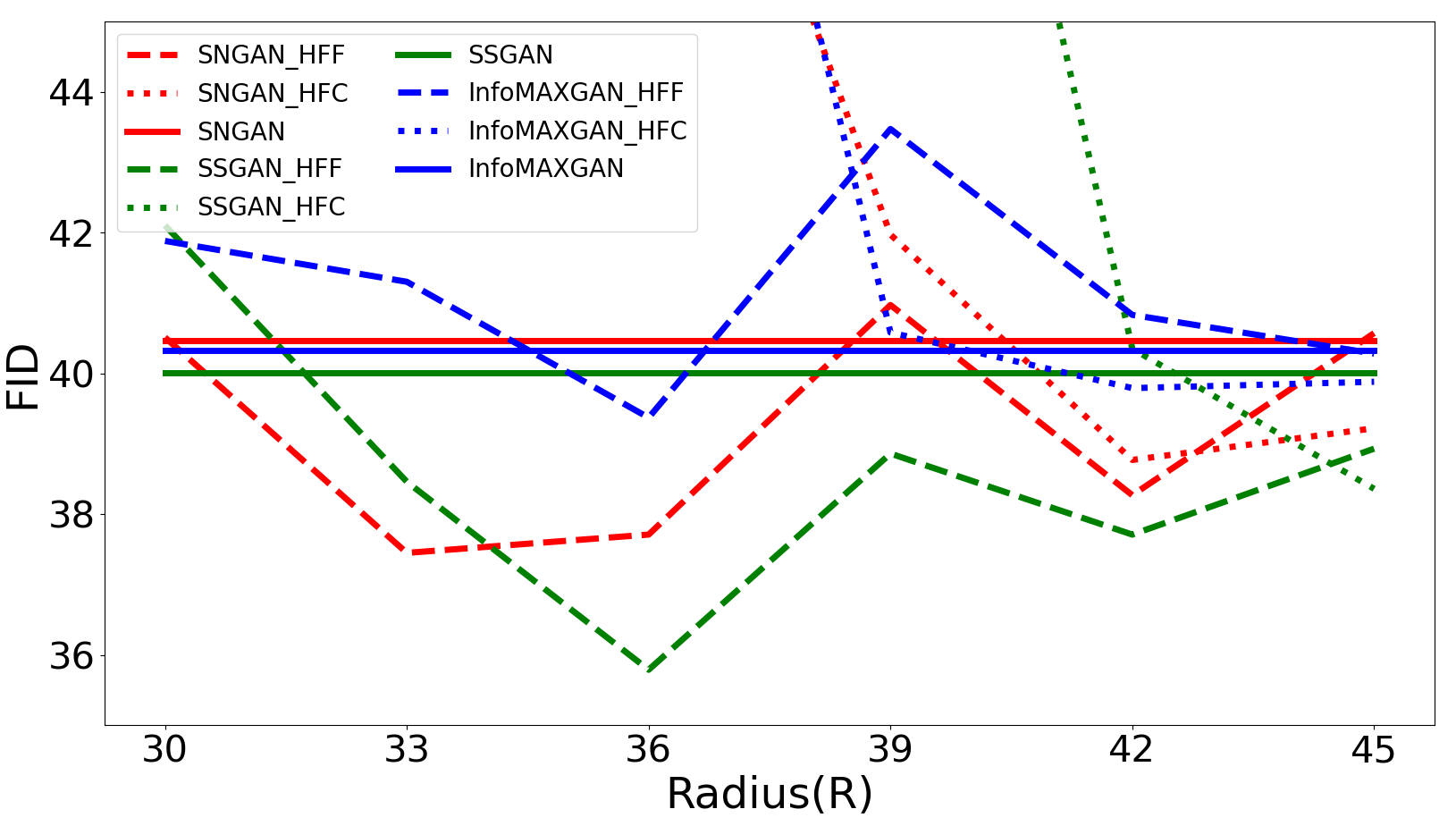
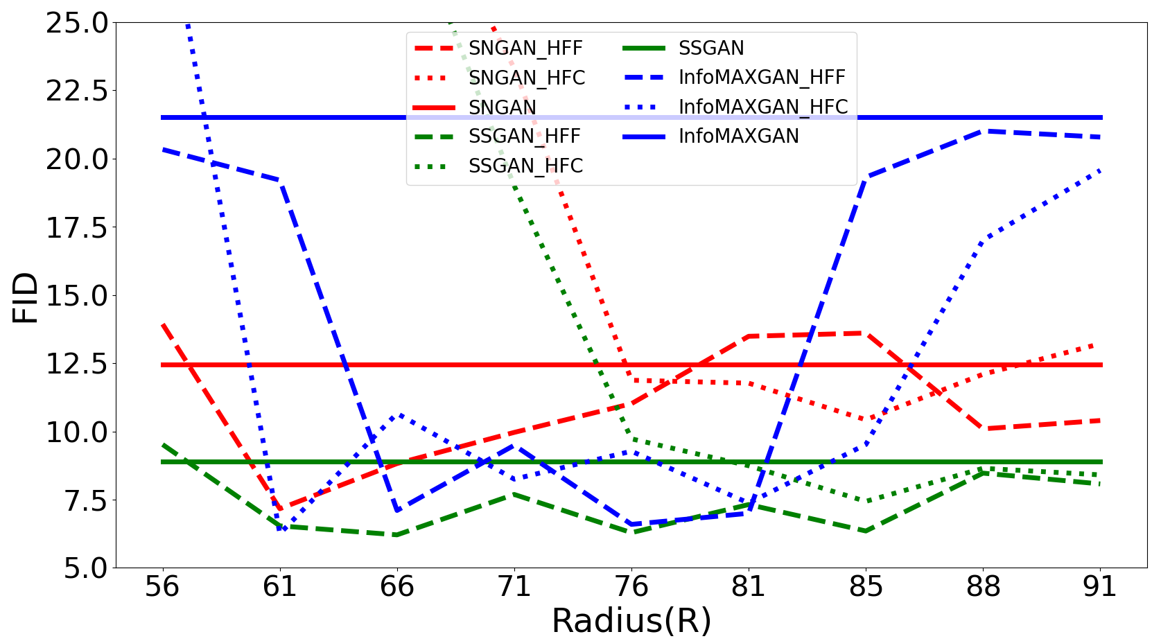
Radius (R) is an important parameter to control the range of frequency during GANs training. Here, different R settings are evaluated on four datasets333Both CIFAR-10 and CIFAR-100 have the same resolution, so we only demonstrate the results on CIFAR-10, STL-10, LSUN-Bedroom, and CelebA datasets. to investigate their effect on the training of GANs. First, the bias of Radial Power Spectrum between real and generated images on four datasets are demonstrated in Figure 10. Figure 10 illustrates that the bias between real and generated images on a small dataset (CIFAR-10) mainly exists in the high-frequency components. But for big datasets, such as STL-10, LSUN-Bedroom, and CelebA, all-frequency components exist the bias between real and generated images, which introduces uncertainty into the setting of the optimal Radius (R). To investigate the effect of different settings of Radius (R), Figure 9 illustrates the FID of different Radius on four datasets. It is clear that: the optimal Radius of HFF444The reason we mainly consider HFF is that HFC can cause model collapse when the Radius is small is set at approximately the same location as the appearance of frequency bias (R=20) on the CIFAR-10 dataset. However, due to the underfitting on complex datasets (STL-10, LSUN-Bedroom, and CelebA), the frequency bias exists in the whole frequency domain. There is uncertainty in the optimal Radius for different models.
| Method | CIFAR-10 | CIFAR-100 | STL-10 | ||||||
| Time(h) | SNGAN | SSGAN | Time(h) | SNGAN | SSGAN | Time(h) | SNGAN | SSGAN | |
| None | 18.1 | 20.05 | 16.75 | 18.4 | 23.70 | 22.43 | 36.0 | 40.77 | 38.78 |
| HFF | 18.3 | 18.54 | 14.71 | 18.4 | 21.45 | 20.27 | 35.5 | 38.99 | 35.13 |
| HFC | 18.2 | 18.28 | 14.88 | 18.3 | 21.98 | 21.51 | 36.2 | 38.43 | 35.14 |
| SSD | 18.7 | 16.73 | 13.51 | 18.9 | 20.73 | 19.91 | 37.8 | 37.04 | 34.43 |
| SSD+HFF | 19.0 | 15.40 | 12.39 | 21.1 | 19.30 | 18.64 | 40.3 | 35.03 | 32.68 |
| SSD+HFC | 18.9 | 16.01 | 12.88 | 20.9 | 19.68 | 19.25 | 39.8 | 34.43 | 33.12 |
Furthermore, we also demonstrate the whole results under the optimal Radius (R) in Table III. The results demonstrate that the proposed methods improve the performance of GANs on different architectures and datasets. For instance, compared to SNGAN, the improvement in FID of SNGAN-HFF is , , , , from CIFAR-10 (32*32), CIFAR-100 (32*32), STL-10 (48*48), LSUN (64*64) to CelebA (128*128). Similarly, compared to SSGAN, the improvement in FID of SSGAN-HFF is , , , , from CIFAR-10, CIFAR-100, STL-10, LSUN to CelebA. In particular, the improvement on the CelebA dataset is significant and impressive, which is open to interpretation. The motivation of our work is high-frequency difference between real and fake images reduces the fit of the generator to the low-frequency components, which is not beneficial for the GANs training. Based on this hypothesis, it is reasonable to assume that the proposed method will realize better performance on large resolution datasets. Dzanic et al. [9] show that at higher resolutions, the differences in frequency domain between real and fake images are more easily observed. Similarly, Figure 10 also illustrates this phenomenon.
For qualitative comparisons, we present randomly sampled images generated by SSGAN and SSGAN with HFF for CIFAR-10, CIFAR-100, STL-10, LSUN-Bedroom, and CelebA datasets in Section B of Supplementary Materials.
IV-D The Comparison with SSD-GAN
SSD-GAN [11] is also a method related to frequency domain in GANs training, which reveals that frequency missing in the discriminator results in a significant spectrum discrepancy between real and fake images. To mitigate this problem, SSD-GAN boosts a frequency-aware classifier into the discriminator to measure the realness of images in both spatial and spectral domains, which improves the spectral discrimination of discriminator. However, the frequency biases between real and fake images have not been eliminated. In our study, we hypothesize that high-frequency differences make the discriminator focus on high-frequency components excessively, which hinders generator from fitting the important low-frequency components. The results indicate that our methods can be combined with SSD-GAN, which further boosts the performance of GANs.
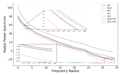
Furthermore, we compare the proposed HFF and HFC with SSD-GAN on multiple datasets, such as CIFAR-10, CIFAR-100, and STL-10 datasets. FID scores and the training time on SNGAN are given in Table IV, where we only use the HFF or HFC in spatial discriminator. The results indicate that the proposed methods improve the performance of GANs with little cost and also boost the performance of SSD-GAN. We also show the Radial Power Spectrum of different SNGAN-based methods on the STL-10 dataset in Figure 11. Compared to SNGAN (None), the low-frequency spectrum discrepancy between images generated by the proposed methods and real data is significantly reduced, where the method ”SSD+HFC” achieves the best performance. Although the proposed method reduces the focus on the high-frequency component, this does not affect the high-frequency fit and even reduces the high-frequency bias.
V Conclusion and Outlook
This paper analyzes the response of discriminator to different-frequency components and indicates that high-frequency bias prevents the fit of the overall distribution, especially the low-frequency components, which is not conducive to the training of GANs. To avoid the high-frequency differences between the generated images and the real images during the GANs training, two frequency operations (HFF and HFC) are introduced in this paper. We provide empirical evidence that the proposed HFF and HFC improve the generative performance with a little cost.
Frequency analysis is an interesting and new perspective on neural networks. Recent works have shown that high-frequency components are related to the generalization and robustness of CNNs. This paper aims for the first pilot study of different frequency components on GANs training. Although significant conclusions and remarkable results have been obtained, the modeling process of GANs for different frequency components is still unclear. In the future, we will verify the frequency principles (DNNs often fit target functions from low to high frequencies during the training) of generators and discriminators, and also explore the relationship between different frequency components and robustness and generalization of GANs training. We hope our work set forth towards a new perspective: Frequency analysis in GANs training.
Acknowledgment
The work is partially supported by the National Natural Science Foundation of China under Grand No.U19B2044 and No.61836011. We are grateful to Chaoyue Wang and Jing Zhang for support of this work.
References
- [1] I. Goodfellow, J. Pouget-Abadie, M. Mirza, B. Xu, D. Warde-Farley, S. Ozair, A. Courville, and Y. Bengio, “Generative adversarial nets,” in Advances in neural information processing systems, 2014, pp. 2672–2680.
- [2] R. Tao, Z. Li, R. Tao, and B. Li, “Resattr-gan: Unpaired deep residual attributes learning for multi-domain face image translation,” IEEE Access, vol. 7, pp. 132 594–132 608, 2019.
- [3] Y. Shen, J. Gu, X. Tang, and B. Zhou, “Interpreting the latent space of gans for semantic face editing,” in Proceedings of the IEEE Conference on Computer Vision and Pattern Recognition, 2020, pp. 9243–9252.
- [4] T. Karras, S. Laine, and T. Aila, “A style-based generator architecture for generative adversarial networks,” in Proceedings of the IEEE conference on computer vision and pattern recognition, 2019, pp. 4401–4410.
- [5] T. Karras, S. Laine, M. Aittala, J. Hellsten, J. Lehtinen, and T. Aila, “Analyzing and improving the image quality of stylegan,” in Proceedings of the IEEE/CVF Conference on Computer Vision and Pattern Recognition, 2020, pp. 8110–8119.
- [6] J. Gu, Y. Shen, and B. Zhou, “Image processing using multi-code gan prior,” in Proceedings of the IEEE/CVF Conference on Computer Vision and Pattern Recognition, 2020, pp. 3012–3021.
- [7] Y.-G. Shin, M.-C. Sagong, Y.-J. Yeo, S.-W. Kim, and S.-J. Ko, “Pepsi++: Fast and lightweight network for image inpainting,” IEEE Transactions on Neural Networks and Learning Systems, 2020.
- [8] M. Khayatkhoei and A. Elgammal, “Spatial frequency bias in convolutional generative adversarial networks,” arXiv preprint arXiv:2010.01473, 2020.
- [9] T. Dzanic, K. Shah, and F. Witherden, “Fourier spectrum discrepancies in deep network generated images,” arXiv preprint arXiv:1911.06465, 2019.
- [10] R. Durall, M. Keuper, and J. Keuper, “Watch your up-convolution: Cnn based generative deep neural networks are failing to reproduce spectral distributions,” in Proceedings of the IEEE/CVF Conference on Computer Vision and Pattern Recognition, 2020, pp. 7890–7899.
- [11] Y. Chen, G. Li, C. Jin, S. Liu, and T. Li, “Ssd-gan: Measuring the realness in the spatial and spectral domains,” in Proceedings of the AAAI Conference on Artificial Intelligence, vol. 35, no. 2, 2021, pp. 1105–1112.
- [12] X. Zhang, S. Karaman, and S.-F. Chang, “Detecting and simulating artifacts in gan fake images,” in 2019 IEEE International Workshop on Information Forensics and Security (WIFS). IEEE, 2019, pp. 1–6.
- [13] J. Frank, T. Eisenhofer, L. Schönherr, A. Fischer, D. Kolossa, and T. Holz, “Leveraging frequency analysis for deep fake image recognition,” arXiv preprint arXiv:2003.08685, 2020.
- [14] T. Miyato, T. Kataoka, M. Koyama, and Y. Yoshida, “Spectral normalization for generative adversarial networks,” arXiv preprint arXiv:1802.05957, 2018.
- [15] H. Wang, X. Wu, Z. Huang, and E. P. Xing, “High-frequency component helps explain the generalization of convolutional neural networks,” in Proceedings of the IEEE/CVF Conference on Computer Vision and Pattern Recognition, 2020, pp. 8684–8694.
- [16] S. Nowozin, B. Cseke, and R. Tomioka, “f-gan: Training generative neural samplers using variational divergence minimization,” in Advances in Neural Information Processing Systems, 2016, pp. 271–279.
- [17] J. H. Lim and J. C. Ye, “Geometric gan,” arXiv preprint arXiv:1705.02894, 2017.
- [18] M. Arjovsky, S. Chintala, and L. Bottou, “Wasserstein gan,” arXiv preprint arXiv:1701.07875, 2017.
- [19] T. Karras, T. Aila, S. Laine, and J. Lehtinen, “Progressive growing of gans for improved quality, stability, and variation,” arXiv preprint arXiv:1710.10196, 2017.
- [20] Z. Li, R. Tao, and B. Li, “Regularization and normalization for generative adversarial networks: A review,” arXiv preprint arXiv:2008.08930, 2020.
- [21] I. Gulrajani, F. Ahmed, M. Arjovsky, V. Dumoulin, and A. C. Courville, “Improved training of wasserstein gans,” in Advances in Neural Information Processing Systems, 2017, pp. 5767–5777.
- [22] Z. Li, “Direct adversarial training for gans,” arXiv preprint arXiv:2008.09041, 2020.
- [23] T. Chen, X. Zhai, M. Ritter, M. Lucic, and N. Houlsby, “Self-supervised gans via auxiliary rotation loss,” in Proceedings of the IEEE Conference on Computer Vision and Pattern Recognition, 2019, pp. 12 154–12 163.
- [24] K. S. Lee, N.-T. Tran, and N.-M. Cheung, “Infomax-gan: Improved adversarial image generation via information maximization and contrastive learning,” in Proceedings of the IEEE/CVF Winter Conference on Applications of Computer Vision, 2020, pp. 3942–3952.
- [25] Z.-Q. J. Xu, Y. Zhang, and Y. Xiao, “Training behavior of deep neural network in frequency domain,” in International Conference on Neural Information Processing. Springer, 2019, pp. 264–274.
- [26] Z.-Q. J. Xu, Y. Zhang, T. Luo, Y. Xiao, and Z. Ma, “Frequency principle: Fourier analysis sheds light on deep neural networks,” arXiv preprint arXiv:1901.06523, 2019.
- [27] N. Rahaman, A. Baratin, D. Arpit, F. Draxler, M. Lin, F. Hamprecht, Y. Bengio, and A. Courville, “On the spectral bias of neural networks,” in International Conference on Machine Learning. PMLR, 2019, pp. 5301–5310.
- [28] I. J. Goodfellow, J. Shlens, and C. Szegedy, “Explaining and harnessing adversarial examples,” arXiv preprint arXiv:1412.6572, 2014.
- [29] Z. J. Xu, “Understanding training and generalization in deep learning by fourier analysis,” arXiv preprint arXiv:1808.04295, 2018.
- [30] Z.-Q. J. Xu, “Frequency principle in deep learning with general loss functions and its potential application,” arXiv preprint arXiv:1811.10146, 2018.
- [31] Y. Zhang, Z.-Q. J. Xu, T. Luo, and Z. Ma, “Explicitizing an implicit bias of the frequency principle in two-layer neural networks,” arXiv preprint arXiv:1905.10264, 2019.
- [32] R. Basri, D. Jacobs, Y. Kasten, and S. Kritchman, “The convergence rate of neural networks for learned functions of different frequencies,” arXiv preprint arXiv:1906.00425, 2019.
- [33] Y. Cao, Z. Fang, Y. Wu, D.-X. Zhou, and Q. Gu, “Towards understanding the spectral bias of deep learning,” arXiv preprint arXiv:1912.01198, 2019.
- [34] M. Tancik, P. P. Srinivasan, B. Mildenhall, S. Fridovich-Keil, N. Raghavan, U. Singhal, R. Ramamoorthi, J. T. Barron, and R. Ng, “Fourier features let networks learn high frequency functions in low dimensional domains,” arXiv preprint arXiv:2006.10739, 2020.
- [35] S. Yamaguchi and S. Kanai, “F-drop&match: Gans with a dead zone in the high-frequency domain,” arXiv preprint arXiv:2106.02343, 2021.
- [36] X. Mao, Q. Li, H. Xie, R. Y. Lau, Z. Wang, and S. Paul Smolley, “Least squares generative adversarial networks,” in Proceedings of the IEEE international conference on computer vision, 2017, pp. 2794–2802.
- [37] A. Krizhevsky, G. Hinton et al., “Learning multiple layers of features from tiny images,” 2009.
- [38] A. Coates, A. Ng, and H. Lee, “An analysis of single-layer networks in unsupervised feature learning,” in Proceedings of the International Conference on Artificial Intelligence and Statistics, 2011, pp. 215–223.
- [39] F. Yu, A. Seff, Y. Zhang, S. Song, T. Funkhouser, and J. Xiao, “Lsun: Construction of a large-scale image dataset using deep learning with humans in the loop,” arXiv preprint arXiv:1506.03365, 2015.
- [40] M. Heusel, H. Ramsauer, T. Unterthiner, B. Nessler, and S. Hochreiter, “Gans trained by a two time-scale update rule converge to a local nash equilibrium,” Advances in Neural Information Processing Systems, vol. 30, pp. 6626–6637, 2017.
- [41] M. Bińkowski, D. J. Sutherland, M. Arbel, and A. Gretton, “Demystifying mmd gans,” arXiv preprint arXiv:1801.01401, 2018.
- [42] T. Salimans, I. Goodfellow, W. Zaremba, V. Cheung, A. Radford, and X. Chen, “Improved techniques for training gans,” Advances in Neural Information Processing Systems, vol. 29, pp. 2234–2242, 2016.