capbtabboxtable[][\FBwidth]
Exploring the Generalizability of Spatio-Temporal Traffic Prediction: Meta-Modeling and an Analytic Framework
Abstract
The Spatio-Temporal Traffic Prediction (STTP) problem is a classical problem with plenty of prior research efforts that benefit from traditional statistical learning and recent deep learning approaches. While STTP can refer to many real-world problems, most existing studies focus on quite specific applications, such as the prediction of taxi demand, ridesharing order, traffic speed, and so on. This hinders the STTP research as the approaches designed for different applications are hardly comparable, and thus how an application-driven approach can be generalized to other scenarios is unclear. To fill in this gap, this paper makes three efforts: (i) we propose an analytic framework, called STAnalytic, to qualitatively investigate STTP approaches regarding their design considerations on various spatial and temporal factors, aiming to make different application-driven approaches comparable; (ii) we design a spatio-temporal meta-model, called STMeta, which can flexibly integrate generalizable temporal and spatial knowledge identified by STAnalytic, (iii) we build an STTP benchmark platform including ten real-life datasets with five scenarios to quantitatively measure the generalizability of STTP approaches. In particular, we implement STMeta with different deep learning techniques, and STMeta demonstrates better generalizability than state-of-the-art approaches by achieving lower prediction error on average across all the datasets.
Index Terms:
spatio-temporal prediction; crowd flow; meta-model1 Introduction
The Spatio-Temporal Traffic Prediction (STTP) problem refers to the problem that resides in many urban predictive applications related to both spatial and temporal human mobility dynamics, e.g., the predictions of taxi demand [1], metro human flow [2], electrical vehicle charging usage [3], and traffic speed [4]. The STTP problems play a vital role in today’s smart city management and organization, e.g., traffic monitoring and emergency response.
Traditionally, STTP is often formulated as a time series prediction problem, where statistical methods such as ARIMA (AutoRegressive Integrated Moving Average) [5, 6] are widely used. In recent years, with the advance of machine learning, especially deep learning techniques, a variety of new models have been developed for STTP. Today, researchers can be quickly overwhelmed by numerous STTP related papers that continuously emerge in top-tier conferences and journals [1, 4, 7, 8, 9]. However, most efforts focus on the sophisticated application-specific model design and then test their models on limited data of one or few specialized applications, e.g., ridesharing [8], bikesharing [9, 10], and highway traffic speed [4]. Although the proposed models can conceptually be applied to other STTP scenarios, whether the performance can still be as good as their specialized applications remains unclear. In other words, it becomes rather difficult to analyze whether an STTP model can be quickly generalized over various scenarios. Indeed, the generalizability is a fundamental and key property of an STTP model, and significantly determines the potential impact scope. In this regard, it is highly urgent to require a general analytic framework that can help investigate and compare different application-driven STTP models. Furthermore, the insights derived from the analytic framework can guide researchers to justify the generalizability of these models, and then design new models with better generalizability.
To fill this research gap, this paper makes efforts from the following aspects:
1) To make different application-driven STTP approaches comparable, we propose an analytic framework, called STAnalytic, to investigate the STTP approaches from their considered high-level spatial and temporal factors. Particularly, STAnalytic maps an STTP model into a two-level hierarchical analysis process where the first level is spatial and temporal perspective, and the second level is knowledge and modeling perspective. Then, every STTP model can be analyzed as two research questions: (1) “what effort is done from temporal and spatial perspective?”; and (2) “which spatial/temporal knowledge is considered with which modeling techniques?”. This qualitative analysis can provide useful insights about whether an STTP model can be well generalized to various scenarios even before we run quantitative experiments over the model.
2) To elaborate the effectiveness of STAnalytic in terms of helping design generalizable STTP models, we propose a spatio-temporal meta-model, called STMeta, based on the analysis results of the STTP over state-of-the-art in literature [1, 4, 7, 8]. STMeta is a “model of model” (meta-model) which has a hierarchical structure to flexibly and efficiently integrate generalizable temporal and spatial knowledge identified by STAnalytic from literature. With state-of-the-art deep learning techniques such as graph convolution [11] and attention mechanisms [12], we implement three variants of STMeta and verify their generalizable effectiveness via multiple real-life STTP benchmark datasets (listed next).
3) To alleviate the issue that today’s STTP research studies usually conduct experiments on certain specific applications and do not justify the generalizability among various applications quantitatively, we build a set of STTP benchmark datasets including five scenarios, i.e., ridesharing, bikesharing, metro, electric vehicle charging, and traffic speed. The datasets cover ten cities, where the longest time duration spans four years and the largest number of traffic data records is more than 400 million. We have released our code and data repository111https://github.com/uctb/UCTB.
To summarize, this paper makes the following contributions:
1) We develop an analytic framework, namely STAnalytic, following which existing STTP approaches can be qualitatively explored. To the best of our knowledge, this is one of the first studies that propose such an analytic framework for the STTP problem.
2) We design a meta-model called STMeta based on the insights derived from STAnalytic over state-of-the-art research [1, 4, 7, 8]. STMeta can flexibly and efficiently take into account multiple spatial and temporal knowledge for building an STTP model.
3) We build a set of real-life STTP benchmark datasets covering five scenarios and ten cities. The benchmark results verify that STMeta generally outperforms state-of-the-art approaches. After analyzing the results, we provide several design guidelines to develop STTP approaches with better generalizability.
2 Problem and Generalizability
2.1 Problem Formulation
First, we formulate the Spatio-Temporal Traffic Prediction problem. Suppose that there are a set of locations , and for each , it has a historical series of traffic information from time slot to the current slot , denoted as . Then, we want to predict the traffic information for each in the next time slot to minimize,
| (1) |
where is the predicted traffic of in the next time slot , and is the ground truth; the function may have many choices. In this paper, we use RMSE (root mean square error).
2.2 Application Scenarios
STTP is an abstraction of many real-world smart city applications that are reported and studied in the literature:
-
•
Region-based Ridesharing Demand Prediction [8]: With the popularity of ridesharing services, one fundamental problem is to predict how many ridesharing demands will emerge in every area of a city. Usually, a city will be split into a set of equal-size regular regions (e.g., grids of 1km * 1km) [8, 1] or irregular regions (e.g., functional areas split by road network) [13], and then one needs to predict the ridesharing demand for each region in near future.
-
•
Station-based Bikesharing Demand Prediction [9]: Bikesharing is another quickly developed service in many cities nowadays. One major type of bikesharing services builds a set of fixed stations in a city and then users can borrow and return bikes at any of those stations. As each station has a limited number of docks to hold bikes, it is important to predict how many users will borrow or return bikes in near future.
-
•
Other Applications. In literature, a lot of other specific problems can also be converted to STTP problems. Actually, most of them can be categorized to region-based or station-based problems. For example, for taxi flow prediction of a city, the problem is often formulated same as ridesharing demand and the regions are pre-defined [1, 14]; for traffic speed prediction of road segments, the problem formulation is similar to the station-based bikesharing case [15, 16].
2.3 Generalizability
While most prior studies focus on specific applications, this paper aims to explore the generalizability issue in STTP. In particular, we concentrate on two generalizability issues: model generalizability and knowledge generalizability:
Model Generalizability. As different STTP applications involve diverse spatial and temporal knowledge factors, the model generalizability refers to: (1) Regarding different spatial and temporal knowledge factors, is a model generalizable to incorporate diverse factors? (2) By incorporating different factors, can a model be generally competitive to the state-of-the-art models in a variety of applications?
Knowledge Generalizability. With the generalizable model that can incorporate various spatial and temporal knowledge factors, we aim to study the knowledge generalizability issue: Given a certain spatial or temporal knowledge factor, is it generalizable to be effective for various STTP applications?
To address the model generalizability issue, we first propose STAnalytic, an analytic framework to investigate the spatial and temporal factors considered in a specific STTP model, which can facilitate a qualitative analysis of the model’s generalizability. With the spatial and temporal factors identified by STAnalytic in mind, we propose STMeta, a meta-model that can incorporate distinct factors in a unified manner; we verify STMeta’s superiority of generalizability over state-of-the-art models by running an extensive benchmark experiment with ten real-life STTP datasets. Finally, with STMeta, we tackle the knowledge generalizability issue by studying how the importance of different spatial and temporal factors vary with the change of benchmark datasets.
3 STAnalytic: Analytic Framework
We propose an analytic framework, called STAnalytic, with which we can investigate and compare different application-driven STTP models and justify their generalizability.
3.1 Framework Overview
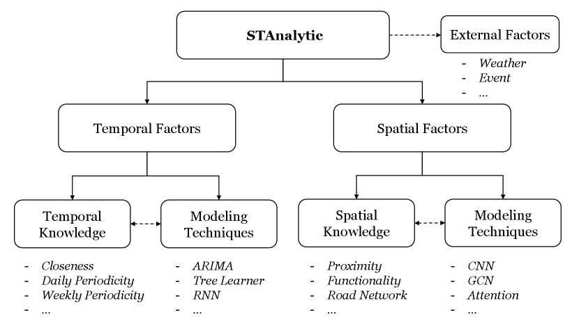
Our framework STAnalytic is illustrated in Figure 1. Overall, the framework considers STTP approaches mainly from two aspects: temporal and spatial factors by answering the following research questions.
RQ1: Does the approach consider temporal and/or spatial factors in predicting traffic?
RQ2: What temporal knowledge factors have been taken into building the approach? For each considered temporal knowledge factor, how does the approach model it?
RQ3: What spatial knowledge factors have been taken into building the approach? For each considered spatial knowledge factor, how does the approach model it?
Regarding RQ1, the STTP approaches based on traditional time-series analysis techniques, such as autoregressive integrated moving average (ARIMA), consider only temporal factors [17, 6]. Other studies leveraging more advanced temporal learning techniques, such as long short-term memory (LSTM) [18, 19], also belong to this temporal-factor-only category. In comparison, more recent STTP approaches mostly consider both temporal and spatial factors explicitly into the model design, especially with state-of-the-art deep learning techniques such as convolution networks [1, 9].
Regarding RQ2 and RQ3, it needs more effort to answer for an STTP approach. To help answer RQ2 and RQ3, the next subsection will review and summarize common temporal and spatial factors that have been considered in the STTP literature. Then, when analyzing a new STTP approach, we can quickly check ‘whether the temporal and spatial factors in consideration belong to our summarized ones’ and ‘whether there is new temporal or spatial knowledge beyond our summarized ones’, so as to answer RQ2 and RQ3.
While spatial and temporal factors are the foundation for traffic prediction, other external factors, e.g., weather [20] and social events [21], may impact traffic patterns prominently, leading to the fourth research question.
RQ4: What external factors have been considered in predicting traffic?
3.2 Temporal and Spatial Knowledge Factors
To help answer RQ2 and RQ3, we investigate the temporal and spatial knowledge that has been well studied in the literature.
3.2.1 Temporal Knowledge Factors and Modeling
Modeling temporal factors has been well studied in STTP, which can be traced back to a very classical research area, time-series analysis [17]. In general, most time series analysis techniques can be applied to STTP; for clarity, we just highlight some most widely used temporal knowledge and its related techniques. The most widely considered temporal knowledge includes temporal closeness, daily periodicity, and weekly periodicity:
Temporal Closeness. One of the most intuitive ways to predict future traffic data is checking back the traffic information of the recent time slots, which is called closeness. In other words, for the models considering closeness (in fact, almost all the models consider closeness), they would take the recent a few time slots’ traffic data as input and then predicts the future.
In literature, many classical statistical methods have been proposed to extract meaningful closeness patterns from the time-series data. The most famous model is perhaps ARIMA [6]. In brief, ARIMA models the traffic of a future slot as a linear combination of the flow of recent slots. As non-linear relations are hard to find with ARIMA, recently researchers started using non-linear models such as tree-based models (e.g., XGBoost [22]) and recurrent neural networks (e.g., LSTM [23, 18]). Note that, regardless of the modeling techniques, if an approach takes recent a few time slots’ traffic data as input, then its temporal consideration factor is closeness.
Daily Periodicity. As human activity has high regularity, the traffic dynamics, whatever the specific application, also often has obvious patterns. The daily periodicity is one of the most significant patterns. For example, on workdays around 8:00 a.m., people get out of home and go to workplaces, leading to the morning rush hours when many types of traffic data (metro, taxis, buses, etc.) will go from the residential area to the working area. In general, if a model considers daily periodicity, it will put the traffic data of previous days at the same time (e.g., the same hour) into the input.
To model the daily periodicity, the seasonal component can be added to ARIMA [5]. Another widely used method is selecting the historical traffic data at the same daily time slot during the last few days into the input, and then use non-linear models to extract daily patterns [1].
Weekly Periodicity. Similar to daily periodicity, the traffic data of certain scenarios may follow weekly periodicity. As an example, Saturday’s traffic will usually be much more similar to last Saturday instead of Friday.
In practice, the difference of modeling weekly periodicity compared to daily periodicity is the temporal lags. For example, suppose we want to predict the traffic data of ‘8:00-8:30 a.m. Oct. 15’. By considering daily periodicity, we take the traffic data of ‘8:00-8:30 a.m. Oct. 14’ as input; in comparison, by considering weekly periodicity, we take that of ‘8:00-8:30 a.m. Oct. 8’ as input. Apart from the different-lag inputs, the modeling techniques are almost the same for weekly and daily periodicity, such as seasonal ARIMA [24].
3.2.2 Spatial Knowledge Factors and Modeling
Compared to temporal knowledge modeling, spatial knowledge modeling recently attracts more interest from researchers as it is more complicated and heterogeneous. For different scenarios, the spatial knowledge may also be different from each other.
Geographic Proximity. ‘Everything is related to everything else. But near things are more related than distant things.’, pointed by Waldo R. Tobler in 1969, has been extensively recognized as the ‘First Law of Geography’. It clearly highlights the importance of proximity in geographic studies. To model geographic proximity in STTP, one widely used method is: for a target location, firstly select the time-series traffic data in near locations into the input, and then leverage methods such as K nearest neighbors to aggregate near locations’ knowledge. More recently, convolution neural networks (CNN) have been widely used to extract geographic proximity patterns, especially for grid-based traffic prediction problems [1]. CNN is good at this because it learns a small parameter matrix (e.g., or ) that can well aggregate a (grid) location’s data together with its nearby (grid) locations. As CNN can be stacked to a very deep structure (e.g., by ResNet [1]), then the geographic proximity pattern can be extracted at different levels.
| Model Name | RQ2: Temporal | RQ3: Spaital | RQ4: External | Modeling Technique (T: Temporal, S: Spatial) | |
| Temporal Only | |||||
| Hamed et al. 1995 [6] | — | close. | — | none | ARIMA (T) |
| Williams et al. 1998 [5] | — | close., daily | — | none | Seasonal ARIMA (T) |
| Williams et al. 2003 [24] | — | close., weekly | — | none | Seasonal ARIMA (T) |
| Ma et al. 2015 [18] | — | close. | — | none | LSTM (T) |
| Temporal & Spatial | |||||
| Zhang et al. 2017 [1] | ST-ResNet | close., daily, weekly | prox. | weather, holiday | Residual Convolution (T, S) |
| Liang et al. 2018 [7] | GeoMAN | close. | func. | none | LSTM (T), Attention (S) |
| Li et al. 2018 [4] | DCRNN | close. | prox. | none | GRU (T), Diffusion Convolution (S) |
| Yu et al. 2018 [15] | STGCN | close. | prox. | none | Gated Convolution (T), Graph Convolution (S) |
| Geng et al. 2019 [8] | ST-MGCN | close., daily, weekly | prox., func., conn. | none | GRU (T), Graph Convolution (S) |
| Guo et al. 2019 [25] | ASTGCN | close., daily, weekly | prox. | none | Attention & Graph Convolution (T, S) |
| Wu et al. 2019 [26] | Graph-WaveNet | close. | prox., data-driven | none | Gated Unit & Dilated Convolution (T), Graph Convolution (S) |
| Bai et al. 2020 [27] | AGCRN | close. | data-driven | none | GRU (T), Graph Convolution (S) |
| Zheng et al. 2020 [28] | GMAN | close. | prox. | none | Attention (T, S) |
| Song et al. 2020 [29] | STSGCN | close. | prox. | none | Graph Convolution (T, S) |
| Yi and Park 2020 [30] | HGC-RNN | close. | func. | holiday | GRU (T), Hypergraph Convolution (S) |
Location Functionality. Functionality is one fundamental character of a location. For example, some locations are residence areas, some locations are shopping areas, and others are industrial areas. Apparently, these characteristics, if obtained, can greatly improve our understanding of these locations’ traffic patterns [31].
In practice, one of the most widely used data sources to characterize the functionality of a location is points-of-interests (POIs) [8] and/or their related social media open check-ins [32, 33]. For example, the number or the distribution of different types of POIs are often used as a spatial feature vector for a location in literature [34, 7]. With such feature vectors, different modeling methods can be leveraged to extract the hidden patterns about the location functionality that are related to the traffic data [35]. Note that, if we have a large amount of historical data among many locations, it is probable that we can directly infer the location functionality from its historical traffic records, so some existing studies also develop methods to use traffic pattern or similarity to describe location functionality [33, 36, 37].
Inter-Location Relationship. In real-world applications, there are many types of spatial relationships between different locations which may indicate traffic patterns. For example, in traffic volume prediction, the locations connected by the same major city road (e.g., circle road in Beijing) will probably have related flow patterns, i.e., connectivity relationship [8]; in metro station flow prediction, the stations in the same metro line may also hold certain correlations in the flow patterns, i.e., same-line relationship.
To model such diverse inter-location relationships, a natural way is to build a graph to link locations with certain relationships. That is, we see each location as a graph node, and then link two location nodes with an edge if they have some relationship (e.g., connected by the same road). Recently, graph convolution techniques have become very powerful tools to extract hidden spatial knowledge from such constructed inter-location relation graphs [8, 9].
It is worth noting that, the geographic proximity and location functionality can also be seen as special instances of inter-location relationships. For geographic proximity, nearby locations can be linked in the graph; for location functionality, the locations with similar functionality can also be connected [8]. This indicates that the inter-location relationship is promising to be generalized to represent various spatial knowledge for STTP.
Data-Driven Modeling without Explicit Knowledge. While spatial patterns of traffic are complicated and heterogeneous in reality, some recent studies attempt to catch spatial knowledge directly by data-driven methods rather than encoding explicit knowledge factors. One representative method is first randomly constructing an inter-location graph, and then applying the graph neural network learning technique to refine the inter-location graph [26, 27]. Generally, the patterns learned by such purely data-driven methods are highly dependent on the amount and quality of the input historical data. Besides, since the inter-location relationship becomes learnable, the overall computation overhead is increased [27].
3.3 External Factors
Besides spatial and temporal factors, researchers have also studied how various external factors may influencer traffic patterns [38]. These research achievements inspire that for a fine-grained traffic prediction, external factors could be a useful extra knowledge source. We list some representative external factors widely studied in the literature.
Weather. Weather information, including temperature, humidity, condition (e.g., rainy, cloudy), etc., would impact human mobility obviously. It has been reported that more than 20% of car accidents are related to weather conditions.222https://ops.fhwa.dot.gov/weather/q1_roadimpact.htm Some researchers have analyzed the correlations of various weather variables and traffic for identifying influential weather factors [20].
Workday/Holiday. Human mobility patterns are diversified between workdays and holidays. For instance, during the Thanksgiving and Christmas holiday, there would be a significant increase on long-distance travels in U.S., leading to heavy congestion on highways [39]. Hence, whether it is a workday or holiday can cause distinct traffic flows.
Event. When certain events happen around a location, the corresponding traffic would be biased from its normal pattern. For instance, when a sports game or concert is held at a stadium, then the passenger flow around the stadium would rapidly rise up, thus impacting the traffic of its nearby metro [21], bikesharing stations [40], etc.
3.4 Analyzing Existing Models
With the preceding issues, now we summarize representative research studies on STTP with STAnalytic. Since in recent years we have witnessed numerous STTP efforts, we thus only select some representative studies from both classical statistical learning and new deep learning methodologies to give an overview.
Regarding RQ1, we select two main streams of traffic prediction studies to analyze with STAnalytic. The first stream only considers the temporal factors with classical statistical methods (e.g., ARIMA) or recent deep learning methods (e.g., LSTM); the second stream leverages the deep learning techniques with both temporal and spatial knowledge in consideration.
As shown in Table I, most of the first stream of works are much older, including Hamed et al. (1995) [6], Williams et al. (1998) [5], and Williams et al. (2003) [24]. All of them take the traffic prediction problem as time-series data analysis and thus solve the problem with ARIMA methods. The results from Williams et al. (1998, 2003) [5, 24] reveal that the daily and weekly periodicity widely exists and thus it is important to consider them in the temporal factors of the traffic prediction. More recently, researchers start leveraging advanced machine learning techniques, such as LSTM, to learn the temporal patterns in traffic prediction [18].
For the second stream of works, we list several representatives [1, 7, 4, 15, 8, 25, 26, 27], which are published in prestigious venues and highly cited. All of these studies apply deep learning techniques into STTP with both temporal and spatial knowledge in consideration. Note that their modeling techniques are distinct (see ‘modeling technique’ in Table I), thus not directly comparable from the technique perspective. However, with STAnalytic, we put more focus on analyzing which types of temporal and spatial knowledge are taken into consideration, and then these studies are clearly comparable as follows:
1) From temporal knowledge (RQ2), ST-ResNet [1], ST-MGCN [8], and ASTGCN [25] consider both closeness and daily/weekly periodicity, while others only consider closeness.
2) From spatial knowledge (RQ3), ST-MGCN [8] considers multiple factors including proximity, functionality, and road connectivity. In comparison, other studies only consider one spatial knowledge of proximity or functionality. Note that Graph-WaveNet [26] and AGCRN [27] use data-driven methods to automatically extract spatial knowledge, which has the potential to outperform specified spatial knowledge with adequate high-quality historical data.
Based on the above comparison, among these approaches investigated by STAnalytic, we can infer that ST-MGCN [8] is probably more generalizable over various scenarios, as it considers more temporal and spatial factors which have been verified effective in literature. That is, the more knowledge, the better prediction. Later in Section 5, we will quantitatively compare most of these representative approaches with real-life STTP datasets.
Another interesting observation from the analysis is based on RQ4. While the literature has shown that various external factors, such as weather and events, can influence traffic patterns, most spatio-temporal traffic prediction methods ignore external factors completely. There may be several reasons. First, how to extract useful external factors, such as events, is a non-trivial problem itself [21]. Second, how external factors impact traffic patterns is highly application-dependent (e.g., the event impacts on metro passenger volume may not be generalized to traffic speed). Then, it is still challenging for general-purpose traffic prediction approaches to incorporate external factors in a unified way for diverse applications. According to this state and making the method comparison fair, we then ignore external factors for all the approaches in our quantitative benchmark experiment (Section 5). Nevertheless, we believe that investigating external factors is a promising research direction for STTP.
4 STMeta: STTP Meta-Model
To show the effect of STAnalytic in guiding the design of generalizable STTP approaches, we propose a meta-model called STMeta, which can consider multiple generalizable spatial and temporal knowledge identified by STAnalytic from literature.
4.1 Design Principles
Before describing the details of STMeta, we first illustrate the key design consideration of STMeta from two aspects:
(1) From the modeling perspective, we aim to fully leverage the state-of-the-art deep learning techniques, which can extract latent features and representations very effectively, especially when we can collect a large amount of historical traffic data with advanced IT infrastructures nowadays.
(2) From the spatio-temporal knowledge perspective, we attempt to consider the representative and generalizable knowledge captured by STAnalytic, so that the knowledge that has already been validated from literature can contribute to our model.
Note that STMeta is a ‘meta-model’ of model: many components of STMeta are not restricted to specific types of learning techniques, but can be implemented by alternative techniques that suit the modeling purpose. Next we will describe the details of STMeta.
4.2 Meta-Model Details
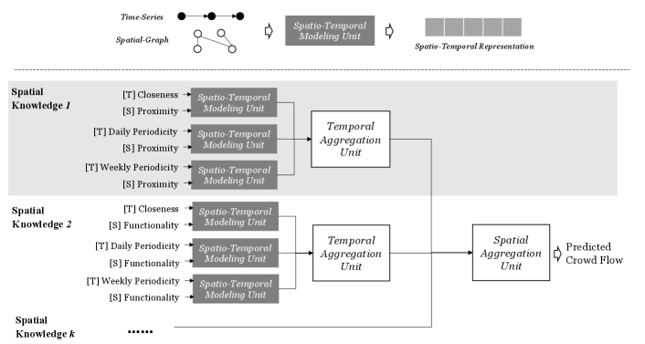
The overview of STMeta is in Figure 2. The key components include the spatio-temporal modeling, temporal aggregation, and spatial aggregation units. We illustrate them as follows.
4.2.1 Spatio-Temporal Modeling
The spatio-temporal modeling part of STMeta includes two key steps. First, we decide which input format is suitable for the temporal and/or spatial knowledge. Second, we need some modeling techniques to extract useful patterns from the temporal and/or spatial knowledge inputs.
To consider the temporal knowledge including closeness, daily periodicity, and weekly periodicity, our model has constructed multiple time-series data regarding different temporal knowledge as the input. Particularly, for closeness, the time-series consists of the traffic data in recent time slots; for daily (or weekly) periodicity, the time-series includes the traffic data in the same time slot of last a few days (or the same weekday-time slot in last a few weeks). We use this input format because it is flexible and can be generalized to other cases. For example, if certain traffic data has bi-weekly/monthly/yearly periodicity patterns, it is easy to implement them into STMeta by adding a corresponding time series.
To consider spatial knowledge, we adopt the inter-location relationship graph as the input because of its generality [8, 9] (Details in ‘Inter-Location Relationship’ of last section). Then, for specific STTP scenarios, researchers can build suitable inter-location relation graphs, e.g., proximity and functionality, to encode the useful spatial knowledge.
Given the temporal and spatial inputs, the key component of our model is the spatio-temporal unit that takes both time-series data (temporal knowledge) and graph structures (spatial knowledge) into account. Recent deep learning research has developed techniques such as graph convolutional long short-term memory (GCLSTM) [9] and diffusion convolutional gated recurrent unit (DCGRU) [4].
(1) GCLSTM: Graph convolution works on a graph where is the vertices and is the adjacency matrix. Let be the normalized Laplace matrix, where is the diagonal degree matrix. The graph convolution can be computed by Chebyshev approximation [11] : where is the - Chebyshev polynomial and is a parameter matrix. To implement GCLSTM, we modify the input and the hidden state of the LSTM unit to a graph convoluted version:
| (2) | |||
| (3) |
The graph convolution part in GCLSTM can consider the spatial information while the LSTM part can take temporal information.
(2) DCGRU: From the design concept, DCGRU is very similar to GCLSTM. That is, DCGRU also re-designs the recurrent neural unit by considering node relations in a graph. The difference is that it uses GRU instead of LSTM, and also replaces the graph convolution operation with the diffusion convolution one.
4.2.2 Spatial and Temporal Knowledge Aggregation
As shown in Figure 2, after the spatio-temporal modeling unit, STMeta will first conduct temporal aggregation to integrate multi-temporal knowledge, and then spatial aggregation to merge multi-spatial knowledge. Similar to the spatio-temporal model unit, there are many candidate deep learning techniques that can be used for temporal and spatial aggregation.
(1) Graph Attention Layer. After firstly being introduced by Google [12], the attention mechanism has quickly been popular in the deep network structure design. One of its main usages is to aggregate multiple features into an integrated one by learning weights for each feature. Particularly, we introduce a method of using the graph attention layer (GAL) [41] to merge multiple features. The input of GAL is a set of node features , , each node being the feature learned from one specific temporal or spatial knowledge (e.g., for three temporal features as closeness, daily and weekly periodicity, has three elements). We first conduct linear transform parametrized by a shared weight matrix , and then perform self-attention on each node using a shared attention parameter :
| (4) |
where represents the importance of to . To make the attention coefficient comparable, we normalize them using softmax:
| (5) |
The output of GAL at can then be represented as
| (6) |
where is the activation function and we use leaky RELU [41]. To make the self-attention process more robust, we add the multi-head mechanism into the model [12] ( is the number of multi-head):
| (7) |
As each node has its own feature after GAL, we then use an average pooling layer to aggregate into a feature vector:
| (8) |
where is the final GAL aggregated feature representation from a set of features .
(2) Concatenation with Dense Layer. Another widely used technique in deep learning to combine multiple features is concatenation. Then, dense layers can be applied to the concatenated features so as to extract useful representations for the target task:
| (9) |
For the temporal or spatial aggregation unit in Figure 2, either of the above two techniques can be selected.
4.2.3 Combing Together
With the spatio-temporal modeling unit and the temporal and spatial aggregation unit, we can then implement concrete STTP approaches following STMeta. Particularly, after spatial aggregation, we can simply stack several dense network layers on the aggregated spatio-temporal representations to predict the future traffic.
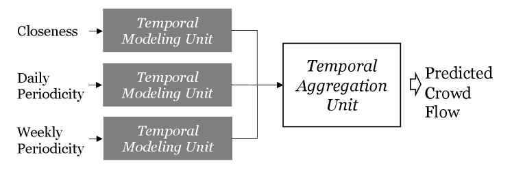
4.2.4 TMeta: Considering Only Temporal Factors
It is worth noting that, following the design principle of STMeta, we can have a simplified version by considering only temporal factors, called TMeta (Figure 3). The temporal modeling unit can be implemented by LSTM [23] or GRU [42]. Later in the benchmark experiments, we will also check how TMeta performs so as to investigate how much improvement can be brought into practice by encoding spatial knowledge.
4.2.5 Comparison with Existing Methods
Compared with the existing methods listed in Table I, STMeta is flexible to incorporate a variety of temporal and spatial factors. In particular, ST-MGCN [8] has also considered multiple temporal and spatial knowledge factors, but its network structure is different from STMeta in temporal modeling. More specifically, ST-MGCN directly combines the weekly, daily, and closeness historical records into one time-series sequence as the input. In comparison, the inputs of STMeta include three types of time-series data regarding closeness, daily periodicity, and weekly periodicity, respectively; thus, STMeta introduces a temporal aggregation unit to combine the three temporal patterns. We think that the design of STMeta may help to learn different temporal patterns more easily, as each temporal pattern (closeness, daily, and weekly periodicity) has its own time-series sequence for dedicated learning.
5 Benchmark Experiment
5.1 Benchmark Datasets
Ten datasets are used in the experiment, covering five scenarios including bikesharing demand (New York City, Washington D.C., and Chicago), ridesharing order (Xi’an and Chengdu)333We conducted ridesharing experiments on both regular (grid) and irregular (administrative district) region-based prediction tasks., metro flow (Shanghai and Chongqing), electric vehicle charging station usage (Beijing), and traffic speed (Los Angeles and Bay Area). The length of a time slot has three different settings, 15/30/60 minutes. Our task is to predict the traffic information at the next time slot. Due to the page limitation, dataset details are described in the online appendix.
5.2 Experiment Settings
5.2.1 Hardware and Training Configurations
The configurations of the experiments are as follows:
Hardware. Our experiment platform is a computation server with AMD Ryzer 9 3900X CPU (12 cores @ 3.80 GHz), 64 GB RAM, and Nvidia RTX 2080Ti GPU (11GB).
Train/Validation/Test Split. We choose the last 10% duration in each dataset as test data, the 10% data before the test for validation. The prediction granularity is set to three settings including 15, 30, and 60 minutes for all datasets.
Training Stopping Criteria. In training, as different datasets and methods need a varying number of epochs for convergence, we thus leverage t-test for the training stopping criteria instead of setting a fixed number of epochs. Particularly, we divide the validation loss of recent epochs (the number of recent epochs is called early stop patience) into two halves. For example, if the early stop patience is 100, then the two halves are last 1-50 epochs and last 51-100 epochs. Then, we perform the independent sample t-test on the validation losses of the two halves. When the p-value is smaller than a threshold (we set it to 0.1), the validation losses of the two halves are statistically different, and thus we continue training. The setting of early stop patience is critical, as a small value may stop training too early when the model is still unstable, while a large value may let early stop become useless and lead to overfitting. With trial-and-error, the early stop patience values of the bikesharing, ridesharing, metro, and EV datasets are set to 200, 1000, 400, and 400, respectively, in our experiments.
5.2.2 Spatio-Temporal Factors in Consideration
We consider the following spatio-temporal factors.
Temporal: We consider temporal closeness, daily, and weekly periodicity in our experiments. For each temporal factor in STMeta, we build one time-series data.
Spatial: For all the datasets, we consider the spatial information including proximity and functionality. For proximity, we build a graph by linking locations whose distance is smaller than a threshold. For functionality, we use the Pearson correlation of the historical traffic data between two locations to indicate their functionality similarity, and link locations with a large correlation. For ridesharing and bikesharing cases, we also build an interaction graph by linking the two locations with frequent interactions (many users go from one location to another) [9]; for metro, we construct a same-line graph by linking the stations in the same line together. The thresholds for building the graphs are shown in Table II. We select these thresholds so that the average number of connections for each node is around 20–30% of the total number of nodes, which performs well in our experiments.
| Bikesharing | Ridesharing | Metro | EV | Speed | |
|---|---|---|---|---|---|
| Prox. | 1,000 | 7,500 | 5,000 | 1,000 | 5,500 |
| Func. | 0 | 0.65 | 0.35 | 0.1 | 0.73 (LA)/0.63 (Bay) |
| Inte. | 40 | 30 | — | — | — |
5.2.3 STMeta Implementations
As shown in Table III, we implement three variants of STMeta by changing the techniques used in spatio-temporal modeling and aggregation units (see Section 4.2).
Specifically, GCLSTM and DCGRU both contain one layer and 64 hidden units; GAL is set to include two heads and 64 hidden units. After temporal and spatial aggregations, we further stack two dense layers with 64 hidden units to generate the prediction output. We choose the optimization algorithm as ADAM [43]; the learning rate is 1e-5. We also implement TMeta (only temporal factors) with LSTM [23].
5.2.4 Benchmark Approaches
We implement a number of benchmark approaches in the literature. These approaches fall into two types, the first only considers the temporal factors and the second considers both temporal and spatial factors.
Approaches with only temporal factors:
-
•
HM (Historical Mean) predicts the traffic according to the mean value of the historical records. We implement two variants of the HM algorithms. The first considers only the recent time slots (closeness), denoted as HM (TC). The second averages recent time slots (closeness), the historical records in the same time of last day (daily periodicity) and last week (weekly periodicity), thus considering multiple temporal factors, denoted as HM (TM).
-
•
ARIMA [24] is a widely used time series prediction model, which mainly considers temporal closeness.
-
•
GBRT (Gradient Boosted Regression Trees) [44] can be applied to predict the traffic for each location. Our GBRT implementation uses historical traffic data as features, not only from recent time slots, but also from last day and last week. Hence, GBRT considers multiple temporal factors.
-
•
XGBoost [22] is similar to GBRT, another widely used tree-based machine learning model.
-
•
LSTM [18] neural networks take the recent time-slot traffic data as inputs (closeness) and predict the future.
Approaches with both temporal and spatial factors:
-
•
ST-ResNet [1] leverages residual convolution networks to consider spatial proximity and also considers temporal closeness, daily and weekly periodicity simultaneously. Note that ST-ResNet can only work for grid-based traffic prediction (ridesharing).
-
•
DCRNN [4] combines diffusion convolution and recurrent networks for capturing spatio-temporal features. The original DCRNN model only considers the temporal closeness and the spatial proximity graph.
-
•
STGCN [15] combines graph convolution and gated convolution units to catch spatial and temporal features, respectively. It considers the temporal closeness and spatial proximity graph.
-
•
GMAN [28] leverages attention mechanisms to model both temporal closeness and spatial proximity patterns for traffic prediction.
-
•
Graph-WaveNet [26] designs a data-driven graph convolution method for adaptively learning spatial knowledge in addition to proximity. For temporal knowledge, it considers only recent traffic data.
-
•
ST-MGCN [8] captures multiple spatial relations with graph convolutions. It also considers temporal closeness, daily and weekly periodicity. Not like STMeta, ST-MGCN concatenates the inputs regarding different temporal factors into one time-series data.
-
•
ARGCN-CDW purely relies on data-driven graph convolution methods for extracting spatial knowledge [27]. Meanwhile, it considers temporal closeness, daily and weekly periodicity same as ST-MGCN.444The original ARGCN [27] considers only temporal closeness, but it is hard to converge in our experiments. By modifying its input as the time-series data combined by closeness, daily and weekly periodicity (same as ST-MGCN), the performance of ARGCN is much improved. We denote this model as ARGCN-CDW.
| ST Unit | TA Unit | SA Unit | |
|---|---|---|---|
| STMeta-GCL-GAL | GCLSTM | GAL | GAL |
| STMeta-GCL-CON | GCLSTM | Concatenation | GAL |
| STMeta-DCG-GAL | DCGRU | GAL | GAL |
| TMeta-LSTM-GAL | LSTM | GAL | — |
| Bikesharing | Ridesharing | Metro | EV | Speed | Overall | |||||||||
| NYC | CHI | DC | XA-gr. | CD-gr. | XA-di. | CD-di. | SH | CQ | BJ | LA | Bay | AvgNRMSE | WstNRMSE | |
| Temporal | ||||||||||||||
| HM (TC) | 5.814 | 4.143 | 3.485 | 10.136 | 14.145 | 52.610 | 74.212 | 824.94 | 673.55 | 1.178 | 12.303 | 5.779 | 2.597 | 7.106 |
| ARIMA (TC) | 5.289 | 3.744 | 3.183 | 9.475 | 13.259 | 47.794 | 65.725 | 676.79 | 578.19 | 0.982 | 11.739 | 5.670 | 2.297 | 6.100 |
| LSTM (TC) | 5.167 | 3.721 | 3.234 | 9.830 | 13.483 | 43.962 | 51.355 | 506.07 | 322.81 | 0.999 | 10.083 | 4.777 | 1.882 | 3.535 |
| HM (TM) | 3.992 | 3.104 | 2.632 | 6.186 | 7.512 | 27.821 | 30.917 | 172.55 | 119.86 | 1.016 | 10.727 | 4.018 | 1.180 | 1.265 |
| XGBoost (TM) | 4.102 | 3.003 | 2.643 | 6.733 | 7.592 | 27.745 | 30.347 | 160.38 | 117.05 | 0.834 | 10.299 | 3.703 | 1.146 | 1.235 |
| GBRT (TM) | 4.039 | 2.984 | 2.611 | 6.446 | 7.511 | 25.654 | 27.591 | 154.29 | 113.92 | 0.828 | 10.013 | 3.704 | 1.111 | 1.202 |
| TMeta-LSTM-GAL (TM) | 3.739 | 2.840 | 2.557 | 5.843 | 6.949 | 23.024 | 25.264* | 163.31 | 102.86 | 0.840 | 8.670* | 3.616 | 1.047 | 1.141 |
| Temporal & Spatial | ||||||||||||||
| DCRNN (TC+SP) | 4.187 | 3.081 | 3.016 | 8.203 | 11.444 | 39.028 | 48.393 | 340.25 | 122.31 | 0.989 | 11.121 | 6.920 | 1.544 | 2.376 |
| STGCN (TC+SP) | 3.895 | 2.989 | 2.597 | 6.150 | 7.710 | 23.916 | 28.940 | 187.98 | 106.16 | 0.859 | 10.688 | 3.472 | 1.121 | 1.313 |
| GMAN (TC+SP) | 4.251 | 2.875 | 2.530 | 7.099 | 13.351 | 28.086 | 30.741 | 193.39 | 117.52 | 0.949 | 10.012 | 3.846 | 1.251 | 1.947 |
| Graph-WaveNet (TC+SP+SD) | 3.863 | 2.812 | 2.403* | 6.541 | 8.162 | 24.101 | 29.406 | 186.82 | 102.75 | 0.930 | 9.463 | 4.135 | 1.129 | 1.305 |
| ST-ResNet (TM+SP) | — | — | — | 6.075 | 7.155 | — | — | — | — | — | — | — | — | — |
| ST-MGCN (TM+SM) | 3.723 | 2.904 | 2.518 | 5.878 | 7.067 | 30.413 | 26.014 | 159.52 | 104.87 | 0.827 | 10.798 | 3.486 | 1.094 | 1.324 |
| AGCRN-CDW (TM+SD) | 3.795 | 2.935 | 2.580 | 8.835 | 10.275 | 35.801 | 38.093 | 658.12 | 287.41 | 0.844 | 10.728 | 3.381* | 1.688 | 4.596 |
| STMeta-GCL-GAL (TM+SM) | 3.518 | 2.695 | 2.405 | 5.871 | 6.858* | 24.127 | 25.669 | 153.17 | 97.87 | 0.831 | 8.834 | 3.514 | 1.024 | 1.070* |
| STMeta-GCL-CON (TM+SM) | 3.507* | 2.739 | 2.404 | 5.829* | 6.873 | 23.244 | 25.296 | 149.05 | 106.41 | 0.807 | 9.147 | 3.552 | 1.027 | 1.123 |
| STMeta-DCG-GAL (TM+SM) | 3.521 | 2.652* | 2.423 | 5.908 | 6.904 | 22.979* | 27.217 | 143.18* | 94.78* | 0.803* | 8.993 | 3.500 | 1.015* | 1.077 |
5.2.5 Metric
We use RMSE (root mean square error) to report the prediction error, as this is the most widely used metric in almost all the STTP research [1, 7, 8, 9, 14].666We have also tested methods in MAE (Mean Absolute Error), and the results are consistent with RMSE. For clarity, we just report RMSE. We also compute two aggregation scores to indicate the overall performance (i.e., generalizability) of an approach ( is the set of all approaches) among all the datasets :
| (10) |
where is the RMSE of approach in dataset . The meaning of the score is the average of the normalized RMSE (normalized by the smallest RMSE for every dataset ). Ideally, if an approach can perform the best among all datasets, then AvgNRMSE is .
| (11) |
If a method is generalizable, its WstNRMSE should also be close to , i.e., in the worst dataset, its performance is still near the best one.
5.3 Experiment Questions
We aim to answer the following questions by experiments.
Q1. Model Generalizability. Can STMeta demonstrate better generalizability than state-of-the-art models? We deem that a model is more generalizable, if it can achieving lower AvgNRMSE and WstNRMSE.
Q2. Knowledge Generalizability. Which temporal or spatial knowledge factors are more generalizable across different datasets? A generalizable factor means that a model considering the factor would exhibit significantly lower AvgNRMSE and WstNRMSE than a model not considering the factor.
5.4 Model Generalizability Results
Table IV, S1 and S2 (Appendix) show our evaluation results for the 60, 30, and 15-minute time slots. For each approach, we mark in the bracket which temporal and/or spatial factors are considered following STAnalytic. The best two results for each dataset are highlighted in bold.
First, we highlight the generalization effectiveness of our STMeta variants over different datasets. From the overall results in Table IV, S1 and S2, we can see that the three different variants of STMeta are usually ranked among the top methods. Particularly, the top method of the three experiments with different time slot lengths is always STMeta variants regarding both AvgNRMSE and WstNRMSE, which verifies the better generalizability of our proposed meta-model STMeta compared to other benchmark approaches. This indicates that our STMeta has the potential to serve as a generalizable STTP meta-model to guide future approach design for a variety of scenarios. Regarding different variants, which one is better depends on the application scenario. This also matches our expectation as we believe that the concrete component implementations in STMeta can have alternative choices (e.g., GCLSTM or DCGRU for the spatio-temporal modeling unit) depending on the scenarios. In the future, if new modeling techniques are proposed, it is possible to implement new STMeta variants.
We also investigate the generalizability of benchmark modeling techniques. To reduce the impact of knowledge variation on our analysis, we compare different approaches with the same spatial and temporal knowledge factors. For ‘TM’ approaches, we find that their overall performance AvgNRMSE ranges from 1.047/1.047/1.086 (TMeta-LSTM-GAL (TM)) to 1.180/1.235/1.246 (HM (TM)) for 60/30/15-minute time slot. On one hand, this validates that advanced modeling techniques can actually improve the model generalizability toward diverse datasets (e.g., state-of-the-art deep learning techniques of TMeta compared to the naive historical mean of HM). On the other hand, it reveals that the improvement brought by modeling technique is around 10-20%, much smaller than the improvement of the extra temporal knowledge (e.g., HM (TC) is worse than HM (TM) by more than 100% in the 60-min experiment).
| Bikesharing | Ridesharing | Metro | EV | Speed | |
| NYC | CD-grid | SH | BJ | LA | |
| C | 4.205 (14.22h/10.53s) | 8.380 (6.72h/0.11s) | 328.81 (7.12h/0.12s) | 3.423 (5.09h/0.20s) | 10.672 (2.16h/0.19s) |
| CD | 3.631 (28.37h/21.54s) | 7.517 (9.23h/0.22s) | 140.67 (10.47h/0.24s) | 0.809 (7.22h/0.40s) | 10.117 (3.35h/0.35s) |
| CDW | 3.521 (34.46h/27.74s) | 6.920 (10.03h/0.28s) | 143.18 (12.46h/0.31s) | 0.803 (7.93h/0.52s) | 8.993 (3.72h/0.45s) |
Another interesting observation is the traditional machine learning model GBRT performs competitively to the state-of-the-art deep learning models in the 15-minute experiment (Table S2). In particular, AvgNRMSE of GBRT in 15-minute prediction is 1.097 (i.e., GBRT is only worse by 9.7% compared to the best model on average). More specifically, in the ridesharing-CD (grid) experiment, GBRT is worse than the best model only by 3.8%, and outperforms many deep models such as Graph-WaveNet and STGCN. Considering the computation resources (computation time), we deem that for STTP with short-length time slots, classical machine learning models may be computation-efficient, i.e., getting relatively good accuracy with significantly lower computation resources, than deep learning methods. This is perhaps because the traffic data relations between continuous time slots become more obvious with the decrease of time slot duration, and classical methods can already capture the relations well.
In addition, we find that the data-driven spatial knowledge modeling (the methods with ‘SD’) performs not stable across different datasets. For instance, AGCRN-CDW (TM+SD) has achieved the smallest prediction error in Speed-Bay (60-minute); however, it performs very poorly in the Metro scenarios (60-minute). Occurring such a large difference is perhaps because extracting spatial knowledge purely from data is of distinct difficulties between datasets. While we believe that data-driven spatial pattern extraction is promising, adopting it in practice still needs caution, as the performance is highly application-dependent.
In summary, by comparing STMeta to various benchmark approaches, we validate its superiority on the generalizable effectiveness over different datasets. Meanwhile, for STTP with short-length time slots, traditional machine learning models, such as GBRT, can also be a good selection thanks to its high computation efficiency and relatively good accuracy.
5.5 Knowledge Generalizability Results
Here, we analyze the results to see how various knowledge factors impact the prediction. Overall, we observe that the best series of approaches regarding knowledge are the ones that consider the largest number of knowledge factors, i.e., the approaches marked as ‘TM+SM’ (multi-temporal and multi-spatial factors). This in fact supports the hypothesis that we have made when we analyze the existing research approaches with STAnalytic (Section 3.4), i.e., the more knowledge, the better prediction. Next, we present a detailed analysis regarding various temporal and spatial factors.
5.5.1 Temporal Knowledge
Regarding the temporal knowledge factors, we first investigate the prediction performance of the ‘temporal’ approaches in Table IV/S1/S2. According to the results, considering more temporal knowledge would improve prediction significantly. For example, in 60-minute prediction (Table IV), HM (TM)’s AvgNRMSE = 1.190; in comparison, HM (TC)’s AvgNRMSE = 2.597, which is much worse than HM (TM). This reveals involving multiple temporal factors indeed enhances the prediction accuracy.
To further elaborate on the impacts of different temporal factors, we conduct an experiment with STMeta by removing certain temporal factors. The results are shown in Table V. We observe that adding periodicity can always enhance the prediction accuracy as human mobility has intrinsic regularity [45]; meanwhile, the training and inference time also increases a bit. Generally, adding both daily and weekly periodicity can bring much improvement, while adding only daily periodicity might be the best (metro, Shanghai). Hence, the temporal periodicity knowledge is often generalizable, while which periodicity performs the best depends on applications.
Besides, with the decrease of the time slot length, the performance gap between ‘TC’ and ‘TM’ methods becomes smaller, indicating that the temporal closeness plays a more important role. For example, in the 60-min experiment, AvgNRMSE of LSTM (TC) and TMeta-LSTM-GAL (TM) are 1.882 and 1.047, respectively, leading to a gap of 0.835; in the 15-min experiment, AvgNRMSE of LSTM (TC) and TMeta-LSTM-GAL (TM) are 1.332 and 1.086, respectively, indicating a gap of only 0.246. This observation signifies that the temporal closeness factor becomes more important when the time slot length is reduced. This also fits our expectation — the correlation between the next 15-minute traffic data and the recent 15-minute should be higher than the correlation between the next 60-minute traffic data and the recent 60-minute, as the time difference of the two continuous slots in the former case is much smaller than the latter case.
5.5.2 Spatial Knowledge
| Bikesharing | Ridesharing | Metro | EV | Speed | |
| NYC | CD-grid | SH | BJ | LA | |
| F | 3.477 (6.40h/5.03s) | 6.878 (2.62h/0.06s) | 148.25 (2.97h/0.06s) | 0.813 (2.93h/0.18s) | 10.149 (1.64h/0.19s) |
| P | 3.509 (6.48h/5.02s) | 6.914 (2.60h/0.07s) | 153.98 (2.96h/0.06s) | 0.835 (2.93h/0.18s) | 10.168 (1.65h/0.19s) |
| I/S | 3.543 (6.40h/5.01s) | 6.879 (2.60h/0.06s) | 151.38 (2.98h/0.06s) | - | - |
| Full | 3.521 (34.46h/27.74s) | 6.904 (10.03h/0.28s) | 143.18 (12.46h/0.31s) | 0.803 (7.93h/0.52s) | 8.993 (3.72h/0.45s) |
Similarly, to analyze how spatial knowledge impacts prediction, we remove some spatial factors from STMeta-DCG-GAL and then compare it to the original STMeta-DCG-GAL (with full spatial knowledge). In particular, for the 60-minute prediction, we implement some variants of STMeta-DCG-GAL with partial spatial information: one of the proximity, functionality, and interaction/same-line graphs. Due to the page limitation, we only show one dataset for each scenario.
Results are shown in Table VI. First, among different spatial graphs, the functionality graph performs always the best. In this regard, we deem that it is more generalizable across different datasets. Besides, the metro, EV, and speed scenarios benefit from the integration of multiple spatial knowledge more significantly than the bikesharing and ridesharing scenarios. For example, in ridesharing, STMeta with full spatial knowledge perform worse than the approach with only one type of spatial knowledge in Chengdu; moreover, training STMeta with full spatial knowledge (i.e., three graphs) costs more than 5 times of the computation hours compared with STMeta with only one spatial graph. Hence, if we blindly add a variety of spatial knowledge graphs into a model, it may degrade both the model effectiveness and efficiency. This inspires that, while generally considering spatial knowledge can improve prediction, selecting and integrating which specific spatial knowledge should be carefully determined for a specific application. Otherwise, it is possible that the overall prediction performance is degraded by adding more spatial knowledge.
5.6 Benchmark Implications
5.6.1 Knowledge vs. Modeling
With the popularity of machine learning, especially deep learning, more and more studies focus on applying novel modeling techniques to the STTP model design, while which temporal or spatial knowledge is considered often lacks detailed analysis. However, our benchmark results indicate that, for STTP model design, it is probable that which part of knowledge in consideration is more important than which modeling technique in use. For example, when we consider complete temporal closeness, daily and weekly periodicity together in the naive historical mean method, HM (TM) can significantly outperform the advanced deep modeling technique with inadequate temporal knowledge, LSTM (TC) that considers only the temporal closeness in all the benchmark scenarios. In a word, regarding the knowledge and modeling techniques, we believe that researchers and practitioners should make more efforts on the knowledge part, i.e., considering more carefully about the temporal and spatial knowledge that may be suitable for the target STTP scenario.
5.6.2 Temporal Knowledge vs. Spatial Knowledge
With the benchmark experiments, we can also compare the relative importance between temporal and spatial knowledge in their generalizability. Overall, we find that purely using temporal knowledge can already achieve competitive generalizability performance across different datasets, compared to the approaches with both temporal and spatial knowledge. For example, TMeta-LSTM-GAL’s AvgNRMSE ranges from 1.047 to 1.086 for 15/30/60-minute prediction experiments. This indicates that the best model with extra spatial knowledge may help improve only 5% beyond temporal knowledge. Specifically, for Bikesharing-CHI (30-minute), TMeta-LSTM-GAL performs the best (tie with STMeta-GCL-CON). This reveals that temporal knowledge can dominate the spatio-temporal factors in some cases. In comparison, as shown in Sec. 5.5.2, adding spatial knowledge does not always improve the prediction accuracy. For different datasets, which spatial knowledge contributes more varies significantly. Hence, our benchmark results reveal that temporal knowledge is more generalizable than spatial knowledge across different STTP scenarios.
5.6.3 Design Guidelines
For the researchers needing to design STTP approaches for their applications, we summarize the following guidelines.
Guideline 0 (most important): Always think deeply about which knowledge should be encoded in the model design before focusing on sophisticated modeling tricks. For a targeted STTP scenario, finding a good set of knowledge suitable for the scenario is a prerequisite and fundamental step before designing model details.
Guideline 1 (Temporal Knowledge): For temporal knowledge, consider temporal closeness, daily and weekly periodicity together. They are perhaps generalized and robust knowledge for various STTP scenarios, as these are fundamental human activity patterns.777Other scenario-specific temporal knowledge may also be carefully designed. For example, if we predict traffic in special seasons such as the Spring Festival Travel Season in China, yearly periodicity is critical.
Guideline 2 (Spatial Knowledge): For spatial knowledge, it needs more careful consideration. Overall, spatial knowledge is not as generalizable as temporal knowledge, whether it is pre-specified or purely learned from data. Hence, instead of simply aggregating all the varieties of spatial knowledge, conduct trial-and-error tests to select the best spatial knowledge combination.
Guideline 3 (STMeta): Our STMeta can be used as a meta-model to integrate multiple temporal and spatial knowledge. With STMeta, researchers only need to consider how to find effective spatial knowledge and encode the knowledge into an inter-location relationship graph.
Guideline 4 (TMeta): To deal with a new STTP problem, we recommend firstly building a TMeta model with only temporal knowledge as an easy-to-implement baseline. This is because temporal knowledge is more generalized than spatial knowledge, and the computation efficiency of TMeta is better than STMeta.
Guideline 5 (Traditional Models): For STTP with short-length time slot settings, the traditional machine learning models with only temporal knowledge, such as GBRT (TM), can be a nice option to trade off the prediction accuracy and computation efficiency.
6 Related Work
The STTP problem is useful for many urban computing scenarios including ridesharing demand, public transportation flow, EV charging station usage [8, 9, 1]. Our paper has investigated some representative studies while there are still many others not mentioned in detail [35, 46, 47, 48, 49, 50]. Due to the page and time limitation, we have not yet analyzed these approaches and re-implemented their methods for evaluation. We will extend our analysis and experimental comparison by selecting more studies and add their model implementations into our code repository.
There are also some research topics related to STTP:
Sensory time-series processing focuses on mining time-series data generated by pervasive sensors, e.g., accelerometers, gyroscopes, and magnetometers [35] to facilitate applications such as mobile sensing [51, 52] and activity recognition [53]. Compared to traffic data, usually the time slot length of the sensory time-series data can be much shorter (e.g., in seconds), and thus the temporal knowledge in consideration can be different. However, we still think that STAnalytic may inspire a similar analysis framework for sensory time-series data.
Individual mobility prediction targets predicting an individual person’s future visiting locations [54, 55]. While this is individual level and STTP involves mostly aggregation level information, there are many commonalities in the leveraged knowledge for building the prediction model. For example, periodicity is recently added by DeepMove [54] into individual mobility prediction and offers a significant improvement. Hence, analyzing the literature on individual mobility prediction following a framework similar to STAnalytic can be interesting and valuable. It is also possible that traffic prediction and individual mobility prediction can learn from each other from such analysis.
7 Conclusion
In this paper, we propose an analytic framework, called STAnalytic, for investigating and comparing existing models for spatio-temporal traffic prediction (STTP). Particularly, with STAnalytic, researchers can investigate and compare what high-level spatial or temporal knowledge is exploited in STTP models, and further justify which model may be generalized to other STTP scenarios. Additionally, we propose a “model of model”, i.e., the meta-model, called STMeta, to flexibly integrate multiple spatio-temporal knowledge identified by STAnalytic from literature. With ten real-life datasets, we have demonstrated that STMeta can generally work well on various scenarios.
Lastly, we re-highlight the novel ideas in this research, which may advance the STTP research promisingly:
(1) Re-framing the fundamental thinking paradigm for STTP research. From the pioneering deep learning-based STTP research in 2017 [1], the STTP area becomes enthusiastic about adopting novel machine and deep learning techniques. Our research reveals that only putting efforts into techniques may not be enough, and we should put more focus on which knowledge factors are considered and whether these factors are generalizable.
(2) Proposing the first (partially) analytical methodology to compare STTP approaches. Generally, no one machine learning technique can win all the time, i.e., the machine learning ‘No free lunch’ theorem.888http://www.no-free-lunch.org/ Most prior STTP papers only rely on experiments over certain datasets to verify performance ‘empirically’. However, whether these approaches can work well for un-tested datasets is still questionable to a certain extent. In comparison, with STAnalytic, our research proposes perhaps the first methodology to compare STTP approaches (partial) ‘analytically’ by considering their considered knowledge factors.
Our future work would include: (1) We will continue updating our project website (https://github.com/uctb/UCTB) to cover new STTP models and datasets. (2) We will extend experimental STTP tasks to multi-step prediction. Given an STTP model, various techniques could be applied to achieve multi-step prediction [56]. It would be interesting to investigate whether (i) there is one single technique that dominantly performs the best, or (ii) different STTP models should cooperate with diverse techniques to achieve the best multi-step prediction performance.
Acknowledgment
This work is supported by NSFC Grant no. 61972008, PKU-Baidu Fund Project no. 2019BD005, and Hong Kong RGC Theme-based Research Scheme no. T41-603/20-R.
References
- [1] J. Zhang, Y. Zheng, and D. Qi, “Deep spatio-temporal residual networks for citywide crowd flows prediction,” in AAAI, 2017, pp. 1655–1661.
- [2] Y. Wei and M.-C. Chen, “Forecasting the short-term metro passenger flow with empirical mode decomposition and neural networks,” Transportation Research Part C: Emerging Technologies, vol. 21, no. 1, pp. 148–162, 2012.
- [3] S. Bae and A. Kwasinski, “Spatial and temporal model of electric vehicle charging demand,” IEEE Transactions on Smart Grid, vol. 3, no. 1, pp. 394–403, 2011.
- [4] Y. Li, R. Yu, C. Shahabi, and Y. Liu, “Diffusion convolutional recurrent neural network: Data-driven traffic forecasting,” in ICLR, 2018.
- [5] B. M. Williams, P. K. Durvasula, and D. E. Brown, “Urban freeway traffic flow prediction: application of seasonal autoregressive integrated moving average and exponential smoothing models,” Transportation Research Record, vol. 1644, no. 1, pp. 132–141, 1998.
- [6] M. M. Hamed, H. R. Al-Masaeid, and Z. M. B. Said, “Short-term prediction of traffic volume in urban arterials,” Journal of Transportation Engineering, vol. 121, no. 3, pp. 249–254, 1995.
- [7] Y. Liang, S. Ke, J. Zhang, X. Yi, and Y. Zheng, “Geoman: Multi-level attention networks for geo-sensory time series prediction,” in IJCAI, 2018, pp. 3428–3434.
- [8] X. Geng, Y. Li, L. Wang, L. Zhang, Q. Yang, J. Ye, and Y. Liu, “Spatiotemporal multi-graph convolution network for ride-hailing demand forecasting,” in AAAI, 2019, pp. 3656–3663.
- [9] D. Chai, L. Wang, and Q. Yang, “Bike flow prediction with multi-graph convolutional networks,” in SIGSPATIAL, 2018, pp. 397–400.
- [10] Z. Yang, J. Hu, Y. Shu, P. Cheng, J. Chen, and T. Moscibroda, “Mobility modeling and prediction in bike-sharing systems,” in MobiSys, 2016, pp. 165–178.
- [11] M. Defferrard, X. Bresson, and P. Vandergheynst, “Convolutional neural networks on graphs with fast localized spectral filtering,” in NeurIPS, 2016, pp. 3844–3852.
- [12] A. Vaswani, N. Shazeer, N. Parmar, J. Uszkoreit, L. Jones, A. N. Gomez, Ł. Kaiser, and I. Polosukhin, “Attention is all you need,” in Advances in neural information processing systems, 2017, pp. 5998–6008.
- [13] J. Sun, J. Zhang, Q. Li, X. Yi, Y. Liang, and Y. Zheng, “Predicting citywide crowd flows in irregular regions using multi-view graph convolutional networks,” IEEE Transactions on Knowledge and Data Engineering, 2020.
- [14] J. Zhang, Y. Zheng, D. Qi, R. Li, X. Yi, and T. Li, “Predicting citywide crowd flows using deep spatio-temporal residual networks,” Artif. Intell., vol. 259, pp. 147–166, 2018.
- [15] B. Yu, H. Yin, and Z. Zhu, “Spatio-temporal graph convolutional networks: a deep learning framework for traffic forecasting,” in IJCAI, 2018, pp. 3634–3640.
- [16] C. Zheng, X. Fan, C. Wang, and J. Qi, “Gman: A graph multi-attention network for traffic prediction,” in AAAI, 2020.
- [17] J. D. Hamilton, Time series analysis. Princeton university press Princeton, NJ, 1994, vol. 2.
- [18] X. Ma, Z. Tao, Y. Wang, H. Yu, and Y. Wang, “Long short-term memory neural network for traffic speed prediction using remote microwave sensor data,” Transportation Research Part C: Emerging Technologies, vol. 54, pp. 187–197, 2015.
- [19] Y. Tian and L. Pan, “Predicting short-term traffic flow by long short-term memory recurrent neural network,” in IEEE International Conference on Smart City/SocialCom/SustainCom, 2015, pp. 153–158.
- [20] A. Koesdwiady, R. Soua, and F. Karray, “Improving traffic flow prediction with weather information in connected cars: A deep learning approach,” IEEE Transactions on Vehicular Technology, vol. 65, no. 12, pp. 9508–9517, 2016.
- [21] M. Ni, Q. He, and J. Gao, “Forecasting the subway passenger flow under event occurrences with social media,” IEEE Transactions on Intelligent Transportation Systems, vol. 18, no. 6, pp. 1623–1632, 2016.
- [22] T. Chen and C. Guestrin, “Xgboost: A scalable tree boosting system,” in KDD, 2016, pp. 785–794.
- [23] F. Gers, J. Schmidhuber, and F. Cummins, “Learning to forget: continual prediction with lstm.” Neural computation, vol. 12, no. 10, pp. 2451–2471, 2000.
- [24] B. M. Williams and L. A. Hoel, “Modeling and forecasting vehicular traffic flow as a seasonal arima process: Theoretical basis and empirical results,” Journal of transportation engineering, vol. 129, no. 6, pp. 664–672, 2003.
- [25] S. Guo, Y. Lin, N. Feng, C. Song, and H. Wan, “Attention based spatial-temporal graph convolutional networks for traffic flow forecasting,” in AAAI, vol. 33, no. 01, 2019, pp. 922–929.
- [26] Z. Wu, S. Pan, G. Long, J. Jiang, and C. Zhang, “Graph wavenet for deep spatial-temporal graph modeling,” in The 28th International Joint Conference on Artificial Intelligence (IJCAI), 2019.
- [27] L. Bai, L. Yao, C. Li, X. Wang, and C. Wang, “Adaptive graph convolutional recurrent network for traffic forecasting,” in 34th Conference on Neural Information Processing Systems, 2020.
- [28] C. Zheng, X. Fan, C. Wang, and J. Qi, “Gman: A graph multi-attention network for traffic prediction,” in AAAI, vol. 34, no. 01, 2020, pp. 1234–1241.
- [29] C. Song, Y. Lin, S. Guo, and H. Wan, “Spatial-temporal synchronous graph convolutional networks: A new framework for spatial-temporal network data forecasting,” in AAAI, vol. 34, no. 01, 2020, pp. 914–921.
- [30] J. Yi and J. Park, “Hypergraph convolutional recurrent neural network,” in KDD, 2020, pp. 3366–3376.
- [31] N. J. Yuan, Y. Zheng, X. Xie, Y. Wang, K. Zheng, and H. Xiong, “Discovering urban functional zones using latent activity trajectories,” IEEE Transactions on Knowledge and Data Engineering, vol. 27, no. 3, pp. 712–725, 2014.
- [32] D. Yang, D. Zhang, Z. Yu, and Z. Yu, “Fine-grained preference-aware location search leveraging crowdsourced digital footprints from lbsns,” in UbiComp, 2013, pp. 479–488.
- [33] L. Wang, X. Geng, X. Ma, F. Liu, and Q. Yang, “Cross-city transfer learning for deep spatio-temporal prediction,” IJCAI, pp. 1893–1899, 2019.
- [34] B. Guo, J. Li, V. W. Zheng, Z. Wang, and Z. Yu, “Citytransfer: Transferring inter-and intra-city knowledge for chain store site recommendation based on multi-source urban data,” Proceedings of the ACM on Interactive, Mobile, Wearable and Ubiquitous Technologies, vol. 1, no. 4, pp. 135:1–135:23, 2018.
- [35] H. Yao, F. Wu, J. Ke, X. Tang, Y. Jia, S. Lu, P. Gong, J. Ye, and Z. Li, “Deep multi-view spatial-temporal network for taxi demand prediction,” in AAAI, 2018, pp. 2588–2595.
- [36] L. Chen, J. Jakubowicz, D. Yang, D. Zhang, and G. Pan, “Fine-grained urban event detection and characterization based on tensor cofactorization,” IEEE Transactions on Human-Machine Systems, vol. 47, pp. 380–391, 2017.
- [37] Z. Fan, X. Song, and R. Shibasaki, “Cityspectrum: a non-negative tensor factorization approach,” in UbiComp, 2014, pp. 213–223.
- [38] C. Zheng, X. Fan, C. Wen, L. Chen, C. Wang, and J. Li, “Deepstd: Mining spatio-temporal disturbances of multiple context factors for citywide traffic flow prediction,” IEEE Transactions on Intelligent Transportation Systems, vol. 21, no. 9, pp. 3744–3755, 2019.
- [39] J. Jun, “Understanding the variability of speed distributions under mixed traffic conditions caused by holiday traffic,” Transportation Research Part C: Emerging Technologies, vol. 18, no. 4, pp. 599–610, 2010.
- [40] L. Chen, D. Zhang, L. Wang, D. Yang, X. Ma, S. Li, Z. Wu, G. Pan, T.-M.-T. Nguyen, and J. Jakubowicz, “Dynamic cluster-based over-demand prediction in bike sharing systems,” in UbiComp, 2016, pp. 841–852.
- [41] P. Veličković, G. Cucurull, A. Casanova, A. Romero, P. Lio, and Y. Bengio, “Graph attention networks,” ICLR, 2018.
- [42] J. Chung, C. Gulcehre, K. Cho, and Y. Bengio, “Empirical evaluation of gated recurrent neural networks on sequence modeling,” arXiv preprint arXiv:1412.3555, 2014.
- [43] D. P. Kingma and J. Ba, “Adam: A method for stochastic optimization,” arXiv preprint arXiv:1412.6980, 2014.
- [44] Y. Li, Y. Zheng, H. Zhang, and L. Chen, “Traffic prediction in a bike-sharing system,” in SIGSPATIAL, 2015, pp. 33:1–33:10.
- [45] C. Song, Z. Qu, N. Blumm, and A. L. Barabási, “Limits of predictability in human mobility,” Science, vol. 327, no. 5968, pp. 1018–1021, 2010.
- [46] J. Ke, H. Zheng, H. Yang, and X. M. Chen, “Short-term forecasting of passenger demand under on-demand ride services: A spatio-temporal deep learning approach,” Transportation Research Part C-emerging Technologies, vol. 85, pp. 591–608, 2017.
- [47] Z. Pan, Y. Liang, W. Wang, Y. Yu, Y. Zheng, and J. Zhang, “Urban traffic prediction from spatio-temporal data using deep meta learning,” in KDD, 2019, pp. 1720–1730.
- [48] Y. Lv, Y. Duan, W. Kang, Z. Li, and F.-Y. Wang, “Traffic flow prediction with big data: A deep learning approach,” IEEE Trans. on Intelligent Transportation Systems, vol. 16, pp. 865–873, 2015.
- [49] J. Zhang, Y. Zheng, J. Sun, and D. Qi, “Flow prediction in spatio-temporal networks based on multitask deep learning,” 2019.
- [50] H. Yao, X. Tang, H. Wei, G. Zheng, and Z. Li, “Revisiting spatial-temporal similarity: A deep learning framework for traffic prediction,” in AAAI, vol. 33, 2019, pp. 5668–5675.
- [51] N. D. Lane, E. Miluzzo, H. Lu, D. Peebles, T. Choudhury, and A. T. Campbell, “A survey of mobile phone sensing,” IEEE Communications Magazine, vol. 48, no. 9, pp. 140–150, 2010.
- [52] J. Zhou and A. K. Tung, “Smiler: A semi-lazy time series prediction system for sensors,” in SIGMOD, 2015, pp. 1871–1886.
- [53] J. Wang, Y. Chen, S. Hao, X. Peng, and L. Hu, “Deep learning for sensor-based activity recognition: A survey,” Pattern Recognition Letters, vol. 119, pp. 3–11, 2018.
- [54] J. Feng, Y. Li, C. Zhang, F. Sun, F. Meng, A. Guo, and D. Jin, “Deepmove: Predicting human mobility with attentional recurrent networks,” in WWW, 2018, pp. 1459–1468.
- [55] Q. Gao, F. Zhou, G. Trajcevski, K. Zhang, T. Zhong, and F. Zhang, “Predicting human mobility via variational attention,” in WWW, 2019, pp. 2750–2756.
- [56] S. B. Taieb and A. F. Atiya, “A bias and variance analysis for multistep-ahead time series forecasting,” IEEE transactions on neural networks and learning systems, vol. 27, no. 1, pp. 62–76, 2015.
Supplementary Tables on Experimental Results
| Bikesharing | Ridesharing | Metro | EV | Speed | Overall | |||||||||
| NYC | CHI | DC | XA-gr. | CD-gr. | XA-di. | CD-di. | SH | CQ | BJ | LA | Bay | AvgNRMSE | WstNRMSE | |
| Temporal | ||||||||||||||
| HM (TC) | 3.206 | 2.458 | 2.304 | 5.280 | 6.969 | 19.893 | 32.098 | 269.16 | 221.39 | 0.768 | 9.471 | 4.155 | 1.865 | 1.909 |
| ARIMA (TC) | 3.178 | 2.428 | 2.228 | 5.035 | 6.618 | 19.253 | 26.131 | 212.01 | 180.53 | 0.755 | 9.230 | 3.936 | 1.667 | 3.687 |
| LSTM (TC) | 3.018 | 2.493 | 2.212 | 4.950 | 6.444 | 18.150 | 23.075 | 195.60 | 104.61 | 0.755 | 7.866 | 3.683 | 1.463 | 2.596 |
| HM (TM) | 2.686 | 2.230 | 1.956 | 4.239 | 4.851 | 16.281 | 17.264 | 108.59 | 74.55 | 0.864 | 9.560 | 3.965 | 1.235 | 1.523 |
| XGBoost (TM) | 2.704 | 2.376 | 1.956 | 4.172 | 4.915 | 15.040 | 16.766 | 81.82 | 69.50 | 0.686 | 8.298 | 3.253 | 1.134 | 1.420 |
| GBRT (TM) | 2.682 | 2.355 | 1.928 | 4.135 | 4.873 | 16.202 | 14.924* | 83.94 | 72.99 | 0.689 | 8.269 | 3.370 | 1.139 | 1.491 |
| TMeta-LSTM-GAL (TM) | 2.511 | 2.133* | 1.927 | 3.847 | 4.678 | 12.687 | 15.324 | 85.19 | 53.18 | 0.686 | 7.436 | 3.231 | 1.047 | 1.130 |
| Temporal & Spatial | ||||||||||||||
| DCRNN (TC+SP) | 2.618 | 2.246 | 2.118 | 4.529 | 6.258 | 19.487 | 22.945 | 116.15 | 65.72 | 0.757 | 8.562 | 6.198 | 1.350 | 2.051 |
| STGCN (TC+SP) | 2.841 | 2.482 | 2.067 | 3.992 | 5.051 | 14.139 | 17.777 | 91.29 | 58.34 | 0.694 | 7.871 | 3.136 | 1.130 | 1.211 |
| GMAN (TC+SP) | 2.792 | 2.336 | 1.836* | 4.026 | 5.293 | 13.994 | 20.157 | 97.58 | 51.37 | 0.764 | 7.276 | 3.688 | 1.142 | 1.351 |
| Graph-WaveNet (TC+SP+SD) | 2.666 | 2.158 | 1.874 | 3.986 | 5.097 | 13.682 | 17.170 | 92.88 | 52.52 | 0.719 | 6.809* | 3.589 | 1.092 | 1.232 |
| ST-ResNet (TM+SP) | — | — | — | 3.903 | 4.673 | — | — | — | — | — | — | — | — | — |
| ST-MGCN (TM+SM) | 2.513 | 2.177 | 1.903 | 3.886 | 4.732 | 13.107 | 15.404 | 88.76 | 50.96 | 0.691 | 8.079 | 3.042 | 1.056 | 1.186 |
| AGCRN-CDW (TM+SD) | 2.830 | 2.565 | 2.074 | 3.958 | 4.753 | 16.921 | 17.982 | 238.99 | 131.55 | 0.688 | 8.575 | 3.022* | 1.440 | 3.171 |
| STMeta-GCL-GAL (TM+SM) | 2.410* | 2.170 | 1.856 | 3.808 | 4.650 | 12.679* | 15.307 | 75.36* | 49.47 | 0.670 | 7.156 | 3.116 | 1.014* | 1.051* |
| STMeta-GCL-CON (TM+SM) | 2.411 | 2.133* | 1.859 | 3.772* | 4.613* | 12.737 | 15.227 | 80.69 | 50.01 | 0.667* | 6.889* | 3.204 | 1.017 | 1.071 |
| STMeta-DCG-GAL (TM+SM) | 2.411 | 2.182 | 1.852 | 3.833 | 4.635 | 12.703 | 15.398 | 77.49 | 48.96* | 0.670 | 7.184 | 3.187 | 1.019 | 1.055 |
| Bikesharing | Ridesharing | Metro | Speed | Overall | |||||||||
| NYC | CHI | DC | XA-gr. | CD-gr. | XA-di. | CD-di. | SH | CQ | LA | Bay | AvgNRMSE | WstNRMSE | |
| Temporal | |||||||||||||
| HM (TC) | 1.903 | 1.756 | 1.655 | 3.155 | 4.050 | 10.022 | 13.530 | 93.81 | 76.67 | 7.150 | 2.967 | 1.461 | 2.443 |
| ARIMA (TC) | 1.874 | 1.784 | 1.689 | 3.088 | 3.948 | 9.664 | 13.138 | 83.54 | 67.11 | 7.028 | 2.869 | 1.394 | 2.138 |
| LSTM (TC) | 1.989 | 1.802 | 1.678 | 3.051 | 3.888 | 9.640 | 12.367 | 80.40 | 55.37 | 6.380 | 2.690 | 1.332 | 1.964 |
| HM (TM) | 1.892 | 1.668 | 1.555 | 2.828 | 3.347 | 8.883 | 10.650 | 49.75 | 45.26 | 8.934 | 3.690 | 1.246 | 1.695 |
| XGBoost (TM) | 1.712 | 1.672 | 1.559 | 2.799 | 3.430 | 8.444 | 10.368 | 47.89 | 35.70 | 6.443 | 2.623 | 1.115 | 1.223 |
| GBRT (TM) | 1.708 | 1.667 | 1.552 | 2.775 | 3.363 | 8.511 | 10.310 | 44.55 | 33.29 | 6.371 | 2.645 | 1.097 | 1.209 |
| TMeta-LSTM-GAL (TM) | 1.818 | 1.623 | 1.540 | 2.917 | 3.286 | 7.932 | 9.815 | 45.88 | 33.34 | 6.156 | 2.544 | 1.086 | 1.168 |
| Temporal & Spatial | |||||||||||||
| DCRNN (TC+SP) | 1.712 | 1.718 | 1.594 | 2.889 | 3.743 | 9.584 | 12.197 | 56.00 | 37.07 | 6.440 | 5.322 | 1.285 | 2.194 |
| STGCN (TC+SP) | 1.738 | 1.806 | 1.630 | 2.789 | 3.453 | 8.402 | 11.070 | 47.40 | 35.19 | 6.236 | 2.493 | 1.125 | 1.237 |
| GMAN (TC+SP) | 1.632* | 1.529 | 1.355* | 2.769 | 3.520 | 8.503 | 11.598 | 49.21 | 36.66 | 6.214 | 3.484 | 1.136 | 1.436 |
| Graph-WaveNet (TC+SP+SD) | 1.644 | 1.460* | 1.357 | 2.764 | 3.442 | 8.066 | 10.571 | 47.84 | 35.04 | 5.270* | 2.780 | 1.065 | 1.169 |
| ST-ResNet (TM+SP) | — | — | — | 2.686 | 3.314 | — | — | — | — | — | — | — | — |
| ST-MGCN (TM+SM) | 1.687 | 1.646 | 1.545 | 2.714 | 3.293 | 7.986 | 9.818 | 46.54 | 32.72 | 6.645 | 2.426* | 1.078 | 1.261 |
| AGCRN-CDW (TM+SD) | 1.836 | 1.883 | 1.745 | 2.722 | 3.296 | 9.386 | 10.127 | 77.06 | 46.95 | 6.709 | 2.453 | 1.246 | 1.882 |
| STMeta-GCL-GAL (TM+SM) | 1.659 | 1.607 | 1.527 | 2.653 | 3.244 | 7.561* | 9.695 | 41.67 | 31.39* | 5.644 | 2.433 | 1.031* | 1.127* |
| STMeta-GCL-CON (TM+SM) | 1.673 | 1.629 | 1.512 | 2.637* | 3.241* | 7.791 | 9.673* | 43.83 | 38.21 | 5.800 | 2.449 | 1.062 | 1.217 |
| STMeta-DCG-GAL (TM+SM) | 1.654 | 1.609 | 1.517 | 2.648 | 3.254 | 7.717 | 9.716 | 40.94* | 36.90 | 5.788 | 2.446 | 1.050 | 1.176 |
Dataset Details
The city area and the locations for each dataset are shown in Figure S1. The dataset statistics are listed in Table S3.
1) Bikesharing. The bikesharing datasets are collected from U.S. open data portals including New York City (NYC, https://www.citibikenyc.com/system-data), Chicago (CHI, https://www.divvybikes.com/system-data), and DC (https://www.capitalbikeshare.com/system-data). The dataset time span for all three cities is more than four years. The total number of historical flow records is around 49 million, 13 million, and 14 million in NYC, Chicago, and DC, respectively, and each record contains the start station, start time, stop station, stop time, etc. We predict the number of bikesharing demands in each station (i.e., the number of bike borrowers).
2) Ridesharing. The ridesharing order datasets are collected from DiDi’s open research collaboration project, including the Chinese cities of Xi’an (XA) and Chengdu (CD). The time span is two months, and the total number of the historical ridesharing orders is around 6 and 8 million for Xi’an and Chengdu, respectively. The order records contain start location, start time, end location, and end time. The location information has longitude and latitude. blue Note that these open data cover only the central area of Xi’an and Chengdu, instead of the whole city area. We use two different strategies to split regions for prediction. (1) Grid (gr.): We divide the area into grids with a size of for each grid, then we predict the number of taxi orders in each grid; (2) District (di.): We split the area according to the administrative district division, and obtain 28 and 25 districts for Xi’an and Chengdu, respectively.
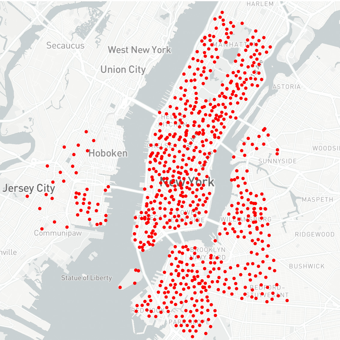
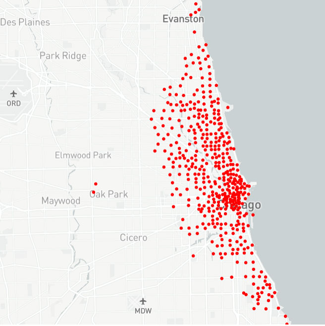
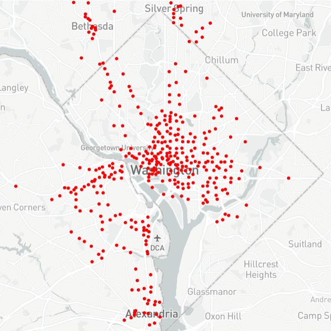
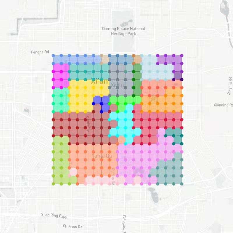
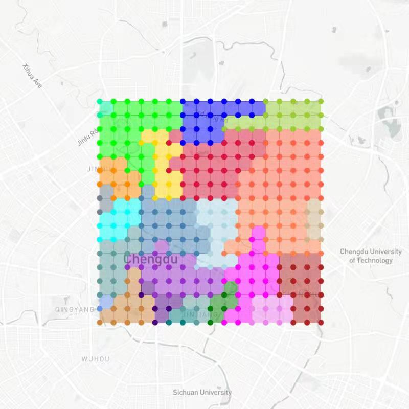
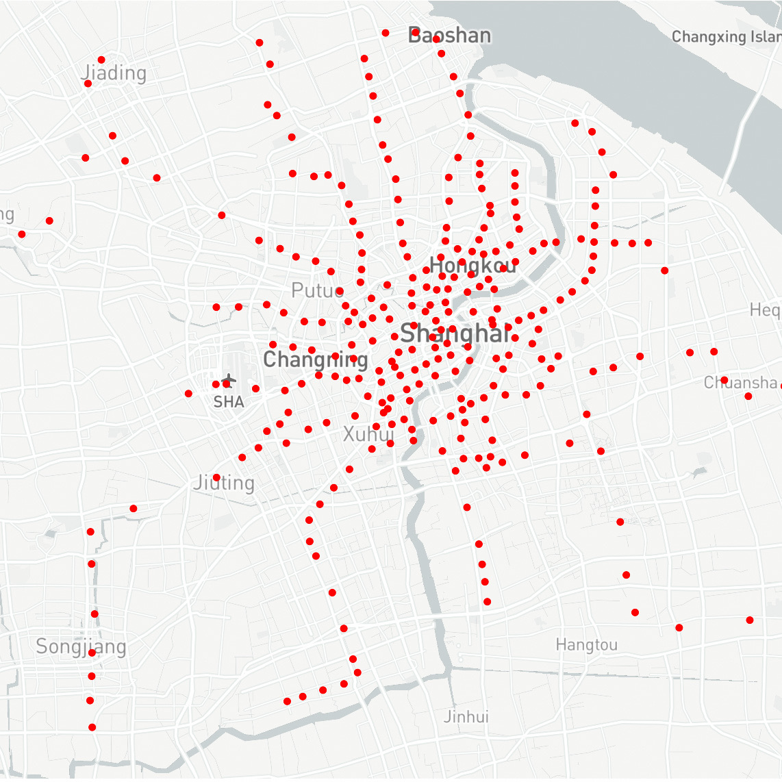
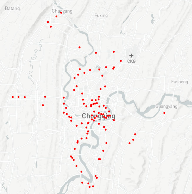
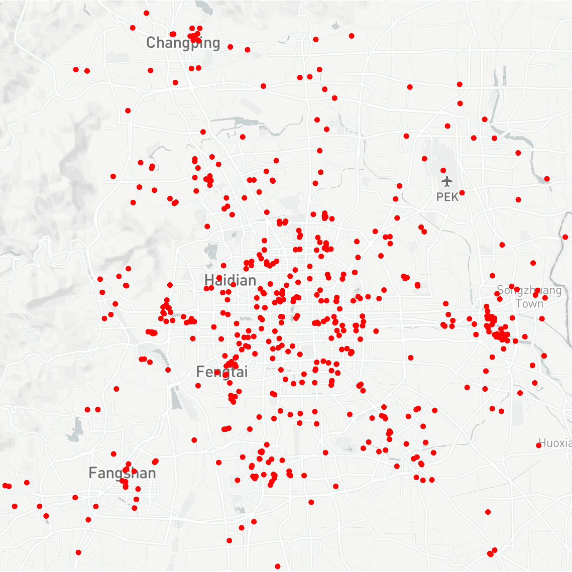
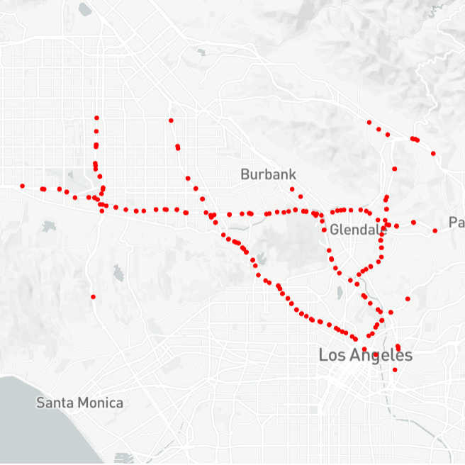
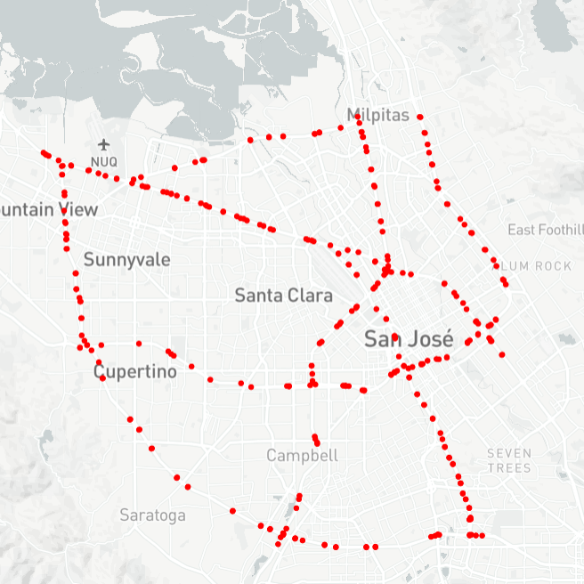
| Bikesharing | Ridesharing | ||||
| NYC | CHI | DC | XA | CD | |
| Time span | 2013.07-2017.09 | 2013.07-2017.09 | 2013.07-2017.09 | 2016.10-2016.11 | 2016.10-2016.11 |
| #Records | 49,100,694 | 13,130,969 | 13,763,675 | 5,922,961 | 8,439,537 |
| #Locations | 820 | 585 | 532 | 256 (grid), 28 (district) | 256 (grid), 25 (district) |
| Metro | EV | Speed | |||
| Shanghai | Chongqing | Beijing | LA | Bay | |
| Time span | 2016.07-2016.09 | 2016.08-2017.07 | 2018.03-2018.08 | 2012.03-2012.06 | 2017.01-2017.07 |
| #Records | 333,149,034 | 409,277,117 | 1,272,961 | 34,272 | 52,128 |
| #Locations | 288 | 113 | 629 | 207 | 325 |
3) Metro. The metro datasets are collected from Shanghai (SH) and Chongqing (CQ). For Shanghai, the time span is three months with around 333 million records; for Chongqing, the time span is one year with around 409 million records. Each metro trip record has the check-in time, check-in station, check-out time, and check-out station. We target predicting the check-in flow amount for all the metro stations.
4) Electrical Vehicle (EV). The EV charging station usage dataset is collected from Beijing (BJ) in the form of stations’ occupation at different time slots, i.e., the number of available and occupied docks. The holder of the stations is one of the largest EV charging station companies in China. The dataset time span is six months and the total number of EV charging station usage records is more than one million. We predict the number of docks in use for each station as this is a demand indicator of the EV charging stations.
5) Speed. The two traffic speed datasets are widely used in STTP research: METR-LA and PEMS-BAY from Los Angeles (LA) County and Bay Area, respectively. In METR-LA, 207 sensors record highway vehicles’ speeds for four months; In PEMS-BAY, there are 325 sensors for six months. Each sensor can be seen as a station, and we predict the traffic speed of each sensor at the next time slot.