Exponential enhancement of quantum metrology using continuous variables
Li Sun
Institute of Fundamental and Frontier Sciences, University of Electronic Science and Technology of China, Chengdu, Sichuan, 610051, China
Xi He
Institute of Fundamental and Frontier Sciences, University of Electronic Science and Technology of China, Chengdu, Sichuan, 610051, China
Chenglong You
Quantum Photonics Laboratory, Department of Physics & Astronomy, Louisiana State University, Baton Rouge, LA 70803, USA
Chufan Lyu
Institute of Fundamental and Frontier Sciences, University of Electronic Science and Technology of China, Chengdu, Sichuan, 610051, China
Bo Li
The Key Laboratory of Mathematics Mechanization, Academy of Mathematics and Systems Science, Chinese Academy of Sciences, Beijing 100190, China
Seth Lloyd
slloyd@mit.eduDepartment of Mechanical Engineering, Massachusetts
Institute of Technology, Cambridge, Massachusetts 02139, USA
Xiaoting Wang
xiaoting@uestc.edu.cnInstitute of Fundamental and Frontier Sciences, University of Electronic Science and Technology of China, Chengdu, Sichuan, 610051, China
(August 18, 2025)
Abstract
Coherence time is an important resource to generate enhancement in quantum metrology. In this work, based on continuous-variable models, we propose a new design of the signal-probe Hamiltonian which generates an exponential enhancement of measurement sensitivity. The key idea is to include into the system an ancilla that does not couple directly to the signal. An immediate benefit of such design is one can expand quantum Fisher information(QFI) into a power series in time, making it possible to achieve a higher-order time scaling in QFI. Specifically, one can design the interaction for a qubit-oscillator Ramsey interferometer to achieve a quartic time scaling, based on which, one can further design a chain of coupled harmonic oscillators to achieve an exponential time scaling in QFI. Our results show that linear scaling in both time and the number of coupling terms is sufficient to obtain exponential enhancement. Such exponential advantage is closely related to the characteristic commutation relations of quadratures.
Quantum metrology aims to study the limitation of the measurement accuracy governed by quantum mechanics and to explore how to achieve better measurement sensitivity with quantum resourcesCaves (1981); Giovannetti et al. (2006). In recent years, quantum metrology has been long pursued due to its vital importance in applied physics, such as gravitational wave detection Schnabel et al. (2010); Danilishin and Khalili (2012); Adhikari (2014), atomic clocks Derevianko and Katori (2011); Schioppo et al. (2017), quantum imaging Kolobov (1999); Dowling and Seshadreesan (2015); Magaña-Loaiza and Boyd (2019). A quantum metrology process includes three steps: preparing probes in a designed initial state; probes evolve under a parameter-dependent Hamiltonian for time ; the measurement of the final state. A well-studied example of parameter estimation is to estimate a parameter introduced in a Hamiltonian with the form of , where is a known Hamiltonian. The sensitivity of estimating this type of parameter scales as , where is the standard deviation of . There are two ways to improve measurement accuracy: either by increasing the coherent interaction time , or by maximizing the standard deviation of through preparing the probe in a special entangled state. Specifically, with quantum entanglement, one can maximize scaling as , where is the number of probes Giovannetti et al. (2006). Accordingly, the estimation sensitivity is considered as the Heisenberg limit, where can be perceived as the quantum parallel resource, and as the quantum serial resource Huelga et al. (1997); Shaji and Caves (2007).
Quantum metrology has been studied for a wide range of systems with quantum resource in parallel schemeGiovannetti et al. (2006, 2004); Boixo et al. (2007, 2008); Woolley et al. (2008); Anisimov et al. (2010); Giovannetti et al. (2011); Thomas-Peter et al. (2011); Hall and Wiseman (2012); Demkowicz-Dobrzański et al. (2012); You et al. (2019); Arvidsson-Shukur et al. (2020); You et al. (2020). For instance, with -body interactions between the probes, a sensitivity limit that scales as can be obtained Boixo et al. (2007), while an exponential scaling can be achieved by introducing an exponentially large number of coupling terms Roy and Braunstein (2008). For quantum resource in serial scheme, in terms of the coherence time ,
many questions remain open. It has been shown that the minimum sensitivity scales as with a time-independent Hamiltonian Huelga et al. (1997); Yuan and Fung (2015); Jones et al. (2020), while scaling can be realized with a time-dependent Hamiltonian Pang and Jordan (2017); Naghiloo et al. (2017). Interesting open questions include: what is the ultimate limit of such enhancement, whether one can achieve sensitivity scaling for arbitrary , or even the exponential scaling with the amount of other physical resources polynomial in ?
Here we show that exponential sensitivity can be efficiently achieved with the number of coupling terms scaling linear with time. Specifically, we study a special type of models with the Hamiltonian in the form , where is coupled with the signal and is an auxiliary Hamiltonian not coupled directly to . Such model utilizes the non-commutativity of and to expand QFI into a power series in , permitting us to obtain higher-order time scaling. In the model of a qubit-harmonic-oscillator(HO) Ramsey interferometer, sensitivity characterized by QFI with time scaling of can be achieved; in the second model with a chain of coupled harmonic resonators, the QFI can obtain an exponential improvement in the measurement accuracy. Remarkably, the second model only requires a polynomial (linear) scaling of coupling terms, which is crucial to justify the efficiency and the effectiveness of exponential enhancement. After all, it is of no surprise to realize exponential enhancement with an exponential amount of physical resource.
Time resource for quantum enhancement. — In quantum metrology, one aims to estimate a parameter encoded in the quantum dynamics from repeated quantum measurements. The variance of the estimation or the measurement sensitivity is bounded by the quantum Cramér-Rao bound (QCRB): , where the QFI corresponds to the minimum quantum measurement sensitivityBraunstein and Caves (1994); Braunstein et al. (1996). The parameter is first encoded into the Hamiltonian , and then into the final state after an evolution time under , with and . Here, is called the symmetric logarithmic derivative (SLD), defined through the relation . Alternatively, QFI can be reformulated in terms of and . Specifically, for pure initial state , we have , where Holevo (2011); Liu et al. (2015). It turns out that such reformulation of FQI is very useful to understand the scheme of quantum enhancement. For example, in the standard setting of quantum metrology where , the above formula gives . Hence, one way to improve QFI is to increase the coherent interaction time . However, due to the decoherence and dephasing effects, cannot be extended arbitrarily long to improve QFI. In comparison, achieving higher-order terms of in QFI is a more efficient and practical method to improve the estimation precision.
In order to find the relationship between and , we consider a general form of on and rewrite into the following polynomial expansion in :
(1)
where is the th-order commutator of and with Kumar (1965); Wilcox (1967); Pang and Brun (2014); Liu et al. (2015).
Thus, we can obtain the expression of QFI:
(2)
Notice that the series in could be of finite length if for some . If are local operators on different subsystems, then for a separable initial state , we have the covariance , and the QFI can be further simplified into
(3)
As shown in Eq. (3), appears in the expression of QFI together with the variance of the th-order commutator in initial state, which provides a possibility to realize higher-order time scaling in QFI.
In the following, we will design the Hamiltonian into the form such that an ancilla probe is introduced to the system and does not couple directly with the signal . We will explore the role played by the commutator in generating higher-order term in coherence time in QFI. In particular, we propose two specific models, the qubit-HO Ramsey interferometer and a chain of coupled harmonic oscillator to investigate the sensitivity enhancement.
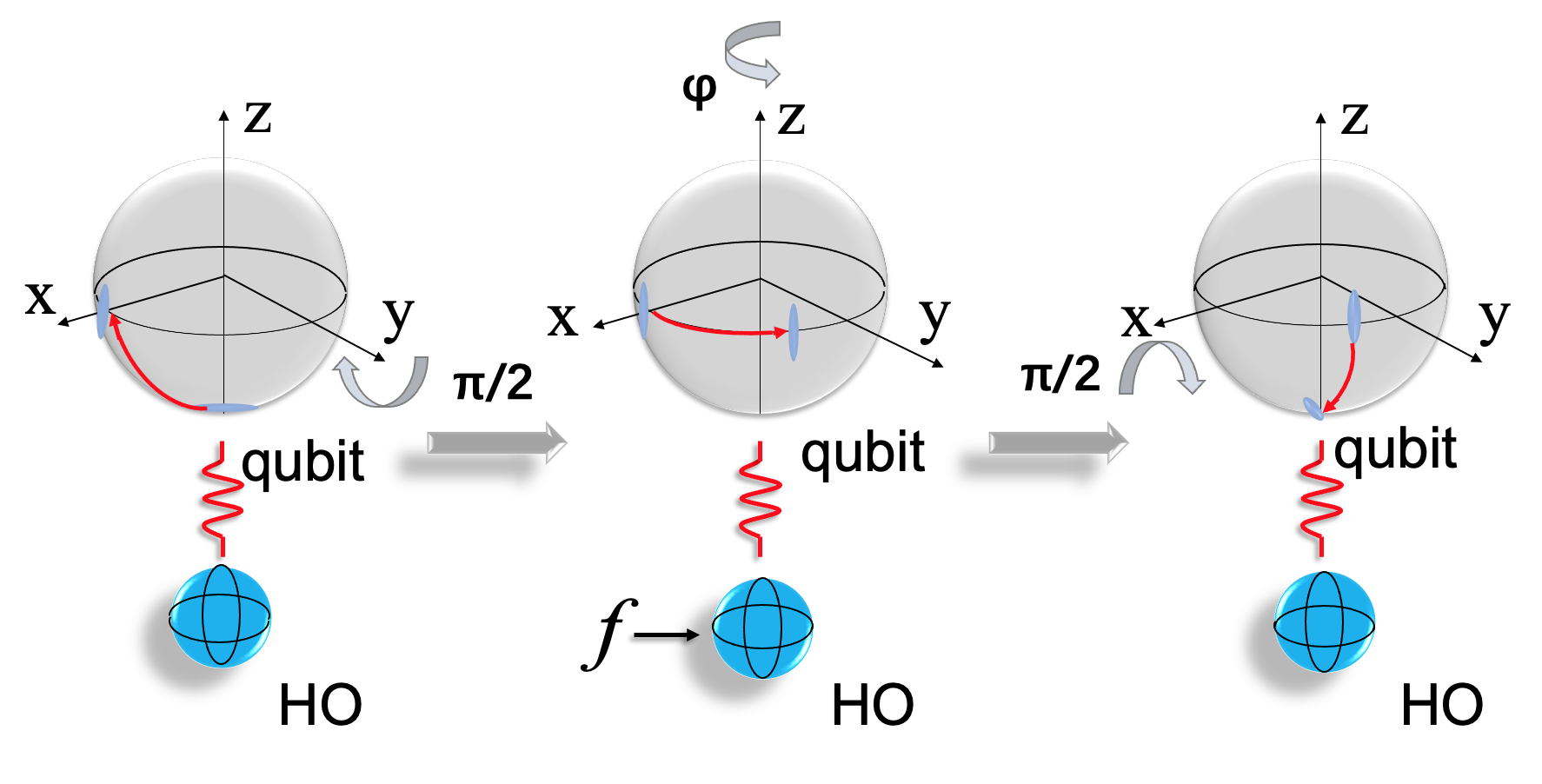
Figure 1: The qubit-HO Ramsey interferometer: the system is composed of a qubit coupled with a HO through the force acting on the HO. The qubit rotates along the -axis firstly. Then is encoded on the HO and the system evolves under , which makes the qubit rotate along the -axis. Lastly, the qubit rotates along the -axis.
Achieving quartic time scaling in QFI. —
We start our analysis with a qubit-HO Ramsey interferometry model. As shown in Fig. 1, the initial state of the qubit and the HO is prepared into a separable state , where is the initial state of HO and () is the ground (excited) state of the qubit. The qubit is subsequently subjected to a pulse along -axis, transforming it into . Afterwards, the system evolves under the Hamiltonian for time , where , , is the Pauli-Z gate, is the annihilation operator and is the qubit-HO coupling strength. Finally, another -pulse around the -axis is applied to the ancilla qubit.
In order to obtain QFI, we calculate commutators as: , and for . Since the initial state of the system is , thus . According to Eq. (3) we calculate QFI as:
(4)
for a separable . In particular, if is the vacuum state, then ; if , where is the squeeze operator and , then for sufficiently large . In both cases, a -scaling of QFI can be achieved. With a strong coupling and relatively long coherent interaction time , a enhancement of can be obtained. As shown in Eq. (4), the higher-order term originates from the non-commutativity between and . Therefore, the non-commutativity in the Hamiltonian could be a useful quantum resource to enhance estimation precision.
The QCRB only gives the optimal lower bound for . We still need to show there exits an optimal quantum measurement to saturate this bound Zhou et al. (2020). One such optimal measurement strategy is given by the measurement observable where is the parity operator on the quantum HO, satisfying . By preparing the HO in the initial state , we can calculate via the error propagation formula:
where and are the variance and the expectation value of in the final state (See details in Supplementary Materials). Thus, a enhancement of can be obtained under such measurement design.
Furthermore, the non-commutativity and entanglement can be used simultaneously to increase estimation precision. We design a system of non-interacting HOs, each of which is coupled with the global force , and an ancila qubit, under the Hamiltonian . By analogy with Eq. (4), if the qubits are in the GHZ state, we can calculate the QFI according to Eq. (2):
(5)
Hence, a quadratic improvement with respect to is obtained in QFI, multiplied by the quartic time scaling, compared with the scheme where the qubits are in a separable state.
Achieving time scaling in QFI. —
Next, we continue the exploration of the choice of the Hamiltonian in order to generate higher-order terms of in QFI, based on the intuition gained from the qubit-HO Ramsey interferometry model. The first attempt is to choose , which gives:
(6)
in Eq. (3). For odd , and for initial state , where is the vacuum state, QFI is further simplified into:
where is even in the summation. Thus we can achieve time scaling in QFI. For instance, for , we have
Nevertheless, it is difficult to experimentally implement such Hamiltonian . Alternatively, we can design to be a chain of coupled HOs with common HO-HO interactions to reach higher-order scaling in QFI.
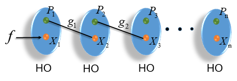
Figure 2: A model containing a chain of coupled HOs, where the signal couples to the first HO via the interaction , and each HO interacts with nearest neighbors via the interaction .
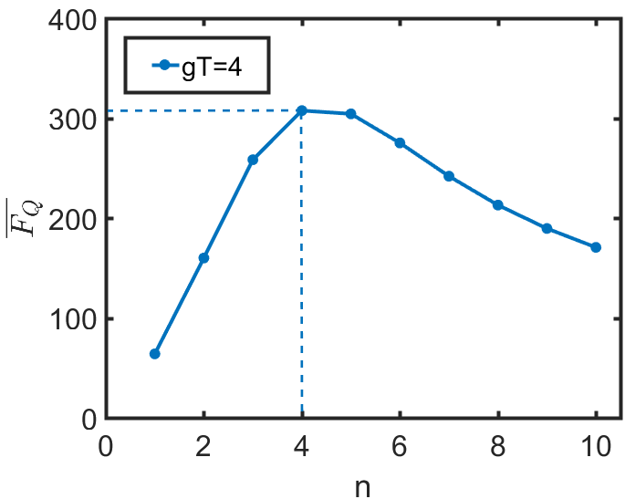
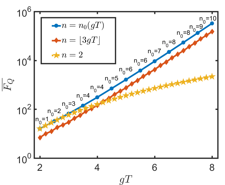
Figure 3: Optimal averaged QFI also demonstrates exponential enhancement. In (a), for , the averaged QFI versus is plotted, with the maximal value achieved at . In (b), the curves for and grow exponentially with , while the curve for grows polynomially with .
Achieving exponential enhancement of QFI. —
As shown in Fig. 2, we design a chain of coupled HOs, where the parameter is coupled with the first HO, and each HO interacts only with its adjacent neighbors, characterized by the total Hamiltonian , with as the coupling constant, and and as the quadratures of the th HO. The signal to be estimated is coupled to the first HO through , and we introduce additional HOs as an ancila for better measurement precision. This model is also known as the bosonic Kitaev-Majorana chain McDonald et al. (2018). Analogous to the previous setup, after the evolution , we can define and calculate the commutators:
(7)
which are local operators on different subsystems. Hence, if the entire system is prepared in a separable initial state, we have . In order to analyze the expression of , we further assume all HOs are prepared in the same initial state, which gives . In this case Eq. (3) is reduced to
(8)
One can further show the following inequality for and :
(9)
Detailed proof of Eq. (9) can be found in the appendix. The intuition behind the proof is, the expression of in Eq. (9) is very similar to the first terms in the Taylor expansion of . The key point is, given the value of , one needs to determine how large has to be so that can scale as up to a constant. It turns out that is sufficient to make QFI scale exponentially with respect to , as long as . Notice that such exponential enhancement of QFI only requires number of HO-HO nearest-neighbor interactions among HOs, which is crucial to justify the efficiency and the effectiveness of the proposal for exponential enhancement. In addition, we can also design an optimal measurement to saturate the QCRB for such exponential scaling of QFI. Specifically, we can choose the parity operator as the measurement observable to reach the exponential enhancement of when and grows linearly under the condition Li et al. (2021).
Achieving the optimal averaged QFI for exponential enhancement —
It turns out that is only sufficient but not necessary or efficient to obtain exponential enhancement of QFI in the previous model. In fact, we can define the averaged QFI per HO as , which is a function of both and . For a fixed , is found to first increase and then decrease as grows, as shown in Fig. 3(a); in other words, there exists an optimal value of to reach to the maximum of for fixed . One can then numerically find the value for different values of . Hence, can be plotted as a curve against in Fig. 3(b), and in the plot it seems to grow exponentially with . For comparison, we also plot and in the same figure. Analogous to the previous discussion, one can rigorously prove that for and , grows exponentially with , as demonstrated in Fig. 3(b); nevertheless, the corresponding is far from being optimal, compared to the curve for . Hence, the condition is only helpful to construct the rigorous proof for exponential enhancement, but not necessary. In practice, should be enough to achieve the exponential behavior. Moreover, keeping growing with is crucial to obtain the exponential enhancement; for a fixed value of , only grows polynomially against , as illustrated in Fig. 3(b).
Conclusion.—As a type of quantum resource, coherent interaction time plays a crucial role in quantum precise measurement. By introducing an auxiliary system which do not couple directly to the signal to be estimated, we can express QFI as a power series in coherence time. For the qubit-oscillator Ramsey interferometer model, QFI has a quartic time scaling; for a chain of coupled harmonic oscillators, with the number of coupling terms growing linearly with time, the corresponding QFI is shown to have an exponential time scaling. Our results suggest that linear scaling in both time and the number of coupling terms is sufficient to obtain exponential enhancement in continuous-variable quantum metrology.
This research was supported by the National Key RD Program of China, Grant No. 2018YFA0306703.
References
Caves (1981)C. M. Caves, Phys. Rev. D 23, 1693 (1981).
Giovannetti et al. (2006)V. Giovannetti, S. Lloyd,
and L. Maccone, Phys. Rev.
Lett. 96, 010401
(2006).
Schnabel et al. (2010)R. Schnabel, N. Mavalvala,
D. E. McClelland, and P. K. Lam, Nat. Commun. 1, 121 (2010).
Danilishin and Khalili (2012)S. L. Danilishin and F. Y. Khalili, Phys. Rev. Lett. 15, 5 (2012).
Derevianko and Katori (2011)A. Derevianko and H. Katori, Rev. Mod. Phys. 83, 331 (2011).
Schioppo et al. (2017)M. Schioppo, R. C. Brown,
W. F. McGrew, N. Hinkley, R. J. Fasano, K. Beloy, T. Yoon, G. Milani, D. Nicolodi,
J. Sherman, et al., Nat. Photon. 11, 48 (2017).
Kolobov (1999)M. I. Kolobov, Rev. Mod. Phys. 71, 1539 (1999).
Dowling and Seshadreesan (2015)J. P. Dowling and K. P. Seshadreesan, J. Lightwave Technol. 33, 2359 (2015).
Huelga et al. (1997)S. F. Huelga, C. Macchiavello, T. Pellizzari, A. K. Ekert, M. B. Plenio, and J. I. Cirac, Phys. Rev.
Lett. 79, 3865
(1997).
Shaji and Caves (2007)A. Shaji and C. M. Caves, Phys. Rev. A 76, 032111 (2007).
Giovannetti et al. (2004)V. Giovannetti, S. Lloyd,
and L. Maccone, Science 306, 1330 (2004).
Boixo et al. (2007)S. Boixo, S. T. Flammia,
C. M. Caves, and J. M. Geremia, Phys. Rev.
Lett. 98, 090401
(2007).
Boixo et al. (2008)S. Boixo, A. Datta,
M. J. Davis, S. T. Flammia, A. Shaji, and C. M. Caves, Phys. Rev. Lett. 101, 040403 (2008).
Woolley et al. (2008)M. Woolley, G. Milburn, and C. M. Caves, New J.
Phys. 10, 125018
(2008).
Anisimov et al. (2010)P. M. Anisimov, G. M. Raterman, A. Chiruvelli, W. N. Plick, S. D. Huver,
H. Lee, and J. P. Dowling, Phys. Rev. Lett. 104, 103602 (2010).
Giovannetti et al. (2011)V. Giovannetti, S. Lloyd,
and L. Maccone, Nat.
Photon. 5, 222
(2011).
Thomas-Peter et al. (2011)N. Thomas-Peter, B. J. Smith, A. Datta,
L. Zhang, U. Dorner, and I. A. Walmsley, Phys. Rev. Lett. 107, 113603 (2011).
Hall and Wiseman (2012)M. J. Hall and H. M. Wiseman, Phys.
Rev. X 2, 041006
(2012).
Demkowicz-Dobrzański et al. (2012)R. Demkowicz-Dobrzański, J. Kołodyński, and M. Guta, Nat. commun. 3, 1 (2012).
Arvidsson-Shukur et al. (2020)D. R. Arvidsson-Shukur, N. Y. Halpern, H. V. Lepage,
A. A. Lasek, C. H. Barnes, and S. Lloyd, Nat. Commun. 11, 1 (2020).
You et al. (2020)C. You, M. Hong, P. Bierhorst, A. E. Lita, S. Glancy, S. Kolthammer, E. Knill, S. W. Nam, R. P. Mirin, O. S. Magana-Loaiza, et al., arXiv preprint arXiv:2011.02454 (2020).
Li et al. (2021)Q. Li, S. Jin, L. Sun, Z.-W. Liu, X. Hou, S. Lloyd, and X. Wang, “Optimal measurement design for
exponential enhancement of quantum metrology,” (2021), upcoming paper.
Measurement design to achieve scaling in measurement uncertainty in the qubit-harmonic-oscillator model
In this work, we use the following definition of the quadratures,
satisfying .
Let’s consider a quantum harmonic oscillator(HO) system coupled with a signal , under the Hamiltonian . Our aim is to measure as accurately as possible. We introduce a probing qubit to interact with the HO through the Hamiltonian . The total Hamiltonian of this qubit-HO model is . Let the initial state of the qubit-HO system to be , its unitary evolution after time is described by:
Thus, the information about is encoded into . If we choose the initial state as a separable state , then the final state after becomes:
The corresponding QFI is:
where and , and for . In particular, if we further choose the initial state of the HO to be , an eigenstate of at position , then , , , and
Hence the minimum measurement uncertainty for such is .
Next, we show there does exist a quantum measurement that can achieve such minimum measurement accuracy. Let’s choose where is the parity operator on the quantum HO satisfying . It turns out that .
For the initial state , the final state becomes:
Hence, the error propagation formula gives:
In practice, we cannot exactly prepare the HO in the unphysical state ; instead, we can prepare the HO in a squeezed state centered as the zero position to approximate . In the case, the final state after becomes
For Fock state , in the position representation, . are real functions: . is an even-function for an even , and an odd-function for an odd . Hence, .
Hence,
The Displacement operator is given by
A few important facts:
Hence, the final state:
If we choose the initial state of HO to be the squeezed vacuum state , then the final state becomes:
For , we have:
where we have used:
Also we have:
For a given value , there exists a sufficiently large such that , , and
Thus, we have achieved the enhancement in .
Proof of the exponential enhancement
Define the following quantities:
We hope to find an appropriate dependence of on such that scales like as increases. First of all, is the Taylor expansion of , satisfying as , for any . Moreover, the larger , the larger is needed for to approximate . One interesting question is, how large should be so that can can approximate reasonably well, i.e., the difference between and can be made arbitrarily small?
By Stirling’s formula and Cauchy–Schwarz inequality, it is easy to show that, for , is sufficient to make sufficiently small and . The next question is whether we can further reduce such quadratic dependence of on to a linear dependence. The answer is yes, as we have the following lemma:
Lemma 1.
For , if is an integer, we have
(1) ;
(2) .
Proof.
For , and , we have
Then, if we choose , and for , we have
According to Stirling’s Formula
we have
Thus, we obtain
implying that for sufficiently large , the difference between and can be made arbitrarily small. Furthermore, it is easy to show that, for ,
From Cauchy–Schwarz inequality, we have:
which gives
On the other hand, for ,
which completes the proof.
∎
Thus, we have shown that, for to be an integer and ,
When is not an integer, we have:
Hence, no matter is an integer or not, we have:
Theorem 1.
For ,
Proof.
For , since , we have
∎
From Eq. (11), we have
Substituting into the expression of and for , we find:
Hence, for and , we have
Moreover, for to be an integer and , analogous to the above discussion, we can prove: