Exponential Kernels with Latency in Hawkes Processes: Applications in Finance
Abstract
The Tick library [tick] allows researchers in market microstructure to simulate and learn Hawkes process in high-frequency data, with optimized parametric and non-parametric learners. But one challenge is to take into account the correct causality of order book events considering latency: the only way one order book event can influence another is if the time difference between them (by the central order book timestamps) is greater than the minimum amount of time for an event to be (i) published in the order book, (ii) reach the trader responsible for the second event, (iii) influence the decision (processing time at the trader) and (iv) the 2nd event reach the order book and be processed. For this we can use exponential kernels shifted to the right by the latency amount. We derive the expression for the log-likelihood to be minimized for the 1-D and the multidimensional cases, and test this method with simulated data and real data. On real data we find that, although not all decays are the same, the latency itself will determine most of the decays. We also show how the decays are related to the latency. Code is available on GitHub at https://github.com/MarcosCarreira/Hawkes-With-Latency.
Keywords: Hawkes processes; Kernel estimations; High-frequency; Order book dynamics; Market microstructure; Python
1 Introduction
It is well known that markets function in response both to external (or exogenous) information - e.g. news - and internal (endogenous) information, like the behavior of market participants and the patterns of price movements. The systematization of markets (synthesized by the Central Limit Order Book) led to two important developments on these responses: order book information is now available in an organized and timely form (which enables the study of intraday patterns in historical data) and algorithms can be deployed to process all kinds of information fast enough to trade (even before the information is received or processed by all the market participants).
That combination increases the importance of understanding how endogenous trading interacts with itself: activity in the order book leads to activity from fast traders which leads to more activity and so on. While the arrival of orders in an order book due to exogenous information can be described as a Poisson process, the interaction of the agents correspond to a self-excitatory process, which can be described by Hawkes processes. The importance of Hawkes processes in finance has been described quite well in [Bacry at al 2015], and recent work by [Euch et al 2016] has established the connection between Hawkes processes, stylized market microstructure facts and rough volatility. More recently, [Bacry et al 2019] improve the Queue-Reactive model by [Huang et al 2015] by adding Hawkes components to the arrival rates.
We start focusing on [Bacry at al 2015], which apply Hawkes processes learners as implemented in the Tick library [tick] to futures. There are two limitations in these applications: for parametric learners the decay(s) must be given and be the same for all kernels, and influences are assumed to be instantaneous. In this short paper we show how to code a parametric learner for an exponential kernel (or kernels in the multivariate case) in which we learn the decay and consider a latency (given). We won’t revisit the mathematical details for the known results; for this, we refer the reader to [Toke 2011] and [Abergel et al 2016]. One of the goals is to show a working Python script optimized at the most by [Numba]; this can be optimized for improved performance. The other goal is to understand what the learned parameters of the kernels mean given the trading dynamics of the BUND futures.
2 One-dimensional Hawkes processes
2.1 Definition
As explained in [Toke 2011], a Hawkes process with an exponential kernel has its intensity described by:
| (1) |
For and :
| (2) |
With stationarity condition:
| (3) |
And unconditional expected value of intensity:
| (4) |
2.2 Maximum-likelihood estimation
Following [Toke 2011]:
| (5) |
Which is computed as:
| (6) |
Defining the function:
| (7) |
The recursion observed by [Ogata et al 1981] is:
| (8) |
And therefore the log-likelihood is:
| (9) |
For and :
| (10) |
And:
| (11) |
2.3 Simulation and learning
Using tick we simulate 100 paths for different end times (100, 1000, 10000) for both the builtin ExpKernel and for a user-defined Time Function that mirrors an ExpKernel:
-
Initialize
Define the kernel function
Define the support
Build the TimeFunction with:
-
n + 1 steps for the time interval
n + 1 evaluations of f for these points
an interpolation mode (e.g. TimeFunction.InterConstRight)
Build a Kernel with HawkesKernelTimeFunc
Define the builtin HawkesKernelExp with parameters
Define the number of simulations
Define the end time
Build the SimuHawkes object with , a kernel and
Build the SimuHawkesMulti object with SimuHawkes and
Simulate SimuHawkesMulti
-
We use minimize from [scipy] with method ’SLSQP’; as pointed out in [Kisel 2017], it can handle both bounds (ensuring positivity of parameters) and constraints (ensuring the stationarity condition). The differences should be calculated at the start of the optimization process and passed to the likelihood function instead of being calculated inside the likelihood function.
-
def :
-
parameters are defined as one argument for the optimization
is one of the SimuHawkesMulti.timestamps
is
is
Define as an array of zeros with the same size as
Keep its first element
Calculate recursively for
Return:
----------------------------------------------------------------------------
Minimize with:
-
bounds on (all must be positive) and
constraint
-
2.4 Kernels with latency
For and , with latency τ:
| (12) |
We can use the same (exponential) function and shift it to the right by the latency:
-
Initialize
Define the kernel function
Define the support
Build the TimeFunction with:
-
n + 1 steps for the time interval
n + 1 evaluations of f for these points
an interpolation mode (e.g. TimeFunction.InterConstRight)
If latency :
-
shift and to the right by
add zeros to the interval
-
Build a Kernel with HawkesKernelTimeFunc
Define the number of simulations
Define the end time
Build the SimuHawkes object with , the kernel and
Build the SimuHawkesMulti object with SimuHawkes and
Simulate SimuHawkesMulti
-
The new likelihoods are defined (for and ) as:
| (13) | ||||
| (14) |
With , and:
| (15) |
Even with the latency , for each we pass . But this enough to slow down the optimization, as observed while testing that the algorithm returns the same results as the previous one for latency zero and seen in Table 1.
-
def :
-
parameters are defined as one argument for the optimization
is one of the SimuHawkesMulti.timestamps
is the series (excluding )
is the series
is the series of arrays for all such that
Define as an array of zeros with the same size as
Keep its first element
Calculate recursively for
Return:
----------------------------------------------------------------------------
Minimize with:
-
bounds on (all must be positive) and
constraint
-
We obtain the following results for 100 paths (parameters , and ) with the total running times in seconds (on a MacBook Pro 16-inch 2019, 2.4 GHz 8-core Intel Core i9, 64 GB 2667 MHz DDR4 RAM):
| End Time | Kernel | Algorithm | runtime (s) | |||||||
|---|---|---|---|---|---|---|---|---|---|---|
| 100 | Builtin | ll | 0. | 535 | 1. | 40 | 0. | 59 | 0. | 87 |
| 100 | Builtin | lllat | 1. | 49 | 1. | 40 | 0. | 59 | 0. | 87 |
| 100 | Custom | ll | 0. | 521 | 1. | 41 | 0. | 63 | 0. | 88 |
| 100 | Custom | lllat | 1. | 6 | 1. | 41 | 0. | 63 | 0. | 88 |
| 1000 | Builtin | ll | 0. | 992 | 1. | 22 | 0. | 60 | 0. | 80 |
| 1000 | Builtin | lllat | 11. | 3 | 1. | 22 | 0. | 60 | 0. | 80 |
| 1000 | Custom | ll | 1. | 13 | 1. | 23 | 0. | 63 | 0. | 81 |
| 1000 | Custom | lllat | 12. | 8 | 1. | 23 | 0. | 63 | 0. | 81 |
| 10000 | Builtin | ll | 6. | 02 | 1. | 20 | 0. | 60 | 0. | 80 |
| 10000 | Builtin | lllat | 143. | 1. | 20 | 0. | 60 | 0. | 80 | |
| 10000 | Custom | ll | 7. | 29 | 1. | 20 | 0. | 62 | 0. | 80 |
| 10000 | Custom | lllat | 181. | 1. | 20 | 0. | 62 | 0. | 80 | |
With latency , we find that we can still recover the parameters of the kernel quite well (still 100 paths):
| End Time | runtime | |||||||
|---|---|---|---|---|---|---|---|---|
| 100 | 1. | 76 | 1. | 41 | 0. | 59 | 0. | 81 |
| 1000 | 15. | 6 | 1. | 26 | 0. | 62 | 0. | 80 |
| 10000 | 223. | 1. | 21 | 0. | 61 | 0. | 79 | |
3 Multidimensional Hawkes
3.1 No latency
For and :
| (16) |
With the recursion now:
| (17) |
And log-likelihood for each node m:
| (18) |
3.2 Latency
For and :
| (19) |
With the recursion now:
| (20) |
And log-likelihood for each node m:
| (21) |
Now there is a choice on how to efficiently select on the recursion: either find the corresponding arrays (which could be empty) for each pair with numpy.extract or find the appropriate for each using numpy.searchsorted and building a dictionary; we chose the latter.
To optimize it further all the arrays are padded so all accesses are on numpy.ndarrays (more details on the code - also see [numpy]).
-
def :
-
parameters are defined as one argument for the optimization
is the index of the time series in the timestamps object
is the array of lengths of all the time series of
-
the timestamps object
is the last timestamp in all of the time series of
-
the timestamps object
is the collection of series for all including
is the collection of collections of series
-
for all and
is the collection of collections of series of arrays
-
for all such that for all and
For each n:
-
Define as an array of zeros with the same size as
Keep its first element
Calculate
-
recursively for
-
Return:
-
----------------------------------------------------------------------------
Minimize with:
-
bounds on (all must be positive)
no constraints for just m
-
A slower optimization can be done for more than one time series in parallel, with the advantage of enforcing symmetries on coefficients by re-defining the input with the same decays for blocks (e.g. on [Bacry et al 2016] instead of 16 different decays we can use 4 decays, as described further down the paper); the algorithm below shows the case where we optimize it for all the time series, but we can modify it to run on bid-ask pairs of time series.
-
def :
-
parameters are defined as one argument for the optimization
is the index of the time series in the timestamps object
is the array of lengths of all the time series of
-
the timestamps object
is the last timestamp in all of the time series of
-
the timestamps object
is the collection of series for all including
is the collection of collections of series
-
for all and
is the collection of collections of series of arrays
-
for all such that for all and
For each m:
-
For each n:
-
Define as an array of zeros with the same size as
Keep its first element
Calculate
-
recursively for
-
Return:
-
Return
-
----------------------------------------------------------------------------
Minimize with:
-
bounds on (all must be positive)
inequality constraints: stationarity condition
equality constraints: symmetries on coefficients
-
3.3 Simulations and learning
With latency and two kernels we get good results (100 paths, method ’SLSQP’):
| End Time | runtime(s) | |||||||||||||||||||||
|---|---|---|---|---|---|---|---|---|---|---|---|---|---|---|---|---|---|---|---|---|---|---|
| Simulated | 0. | 6 | 0. | 2 | 0. | 5 | 0. | 7 | 0. | 9 | 0. | 3 | 1. | 4 | 1. | 8 | 2. | 2 | 1. | 0 | ||
| 100 | 7. | 1 | 0. | 68 | 0. | 28 | 0. | 55 | 0. | 73 | 1. | 03 | 0. | 37 | 1. | 87 | 1. | 93 | 2. | 44 | 2. | 65 |
| 1000 | 67. | 0. | 63 | 0. | 21 | 0. | 52 | 0. | 75 | 0. | 98 | 0. | 31 | 1. | 44 | 1. | 78 | 2. | 18 | 1. | 05 | |
| 10000 | 804. | 0. | 60 | 0. | 20 | 0. | 52 | 0. | 75 | 0. | 97 | 0. | 31 | 1. | 37 | 1. | 76 | 2. | 12 | 1. | 00 | |
4 Results on real data
4.1 Estimation of Slowly Decreasing Hawkes Kernels: Application to High Frequency Order Book Dynamics
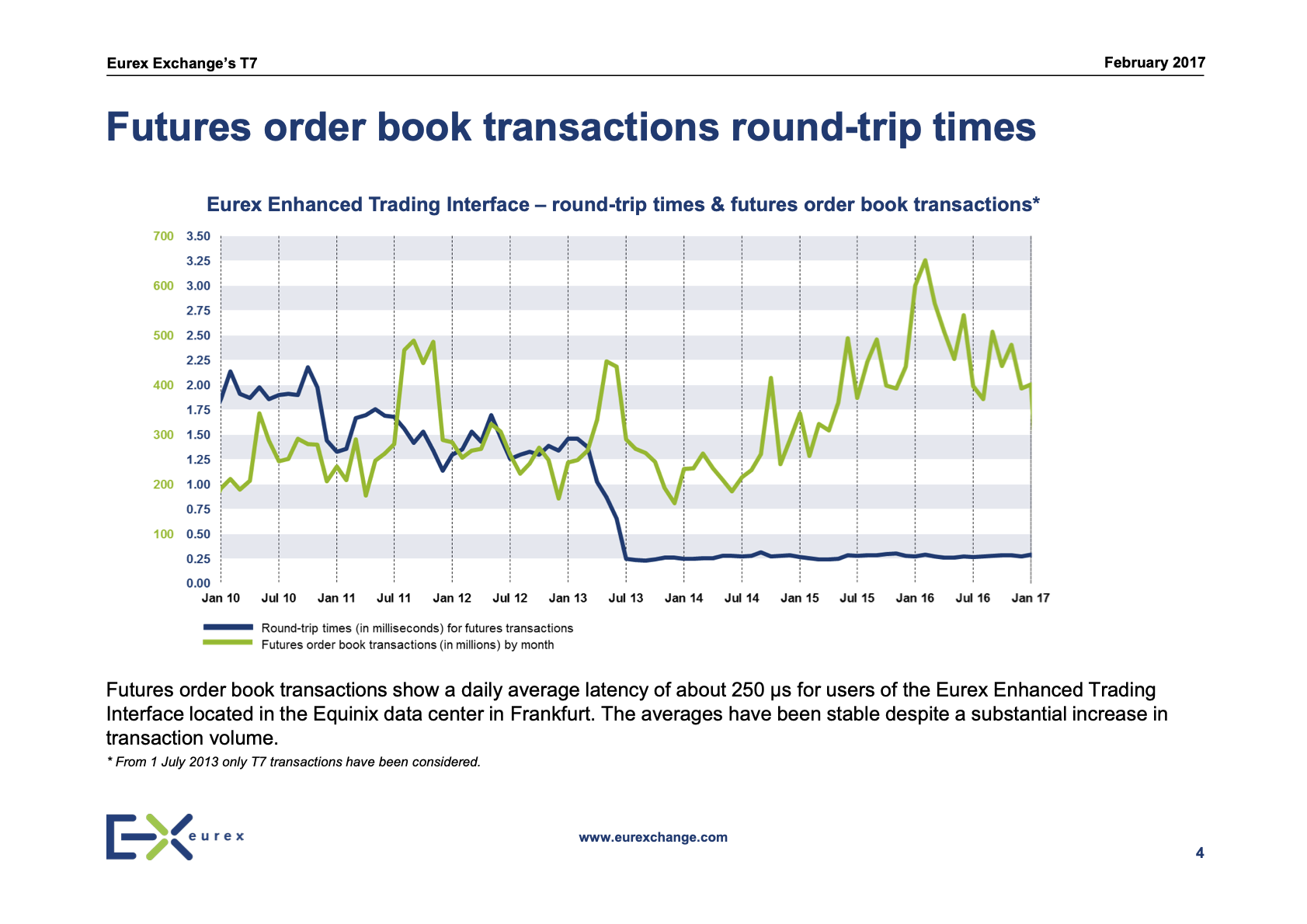
Here one must consider the latency of (as informed in [Eurex 2017]):
We have available data for 20 days (Apr-2014) on events P and T, from 8h to 22h (14 hours on each day), as described in https://github.com/X-DataInitiative/tick-datasets/tree/master/hawkes/bund. Because in some days we have late starts, and because liquidity late at night is not better, we consider events only from 10h to 18h, which represent more than 75% of all events (daily counts available on GitHub).
To get a better idea of the time scales involved, we calculate the descriptive statistics of each time series:
| (events) | 4569 | 4558 | 11027 | 12811 |
| (μs) | 196 | 196 | 147 | 229 |
| (μs) | 241 | 242 | 317 | 471 |
| (μs) | 342 | 340 | 1890 | 11756 |
| (ms) | 14.1 | 13.0 | 159.7 | 183.2 |
| (s) | 2.5 | 2.4 | 1.9 | 1.5 |
| (s) | 16.9 | 17.1 | 7.5 | 6.3 |
| (s) | 6.3 | 6.3 | 2.6 | 2.2 |
And we can see that between 10% and 15% of events within each time series happen less than after the previous event, and therefore should not be considered as being caused by that previous event. We can also see that the average time interval is considerably higher than the median time interval, which means that this distribution is more fat-tailed than an exponential distribution.
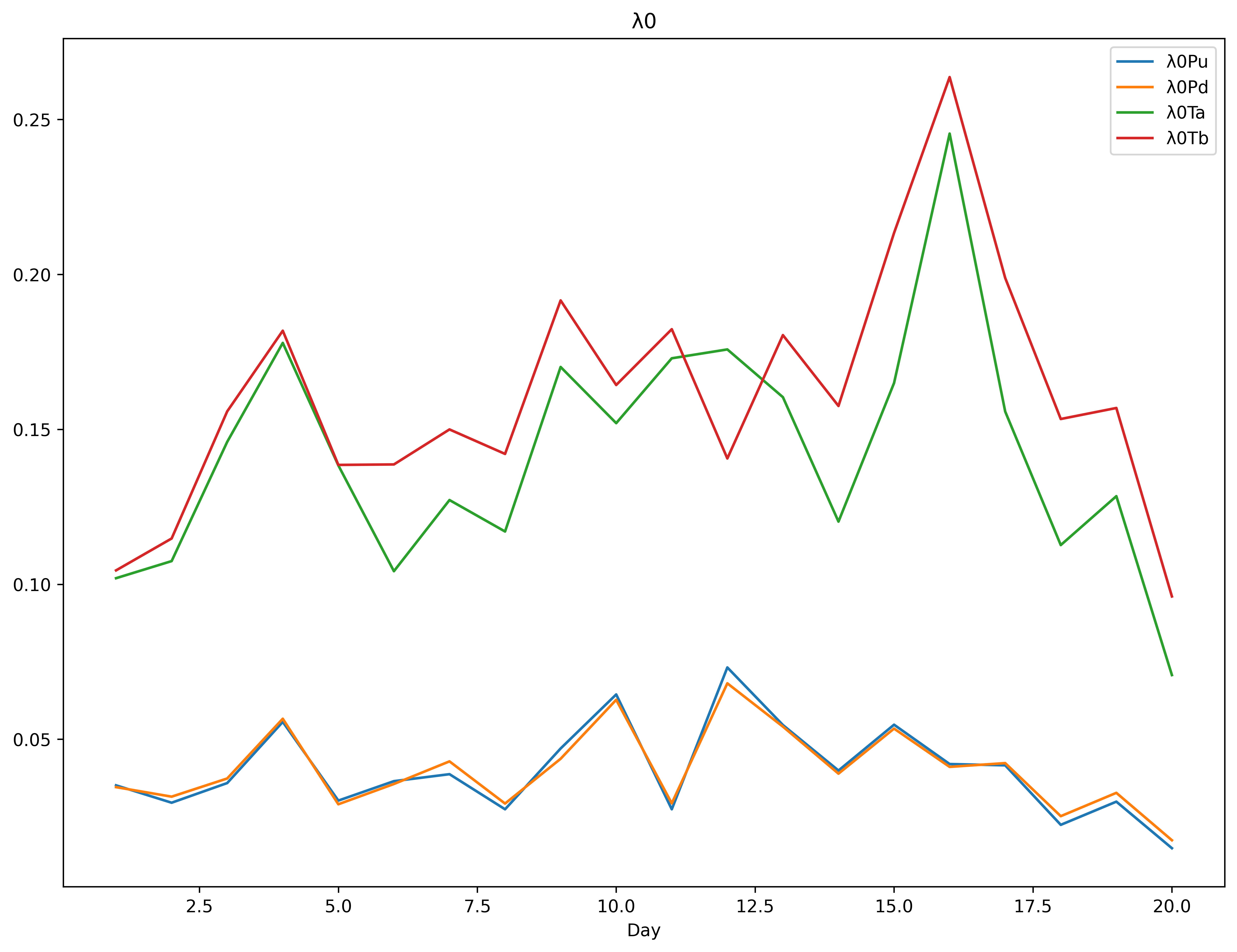
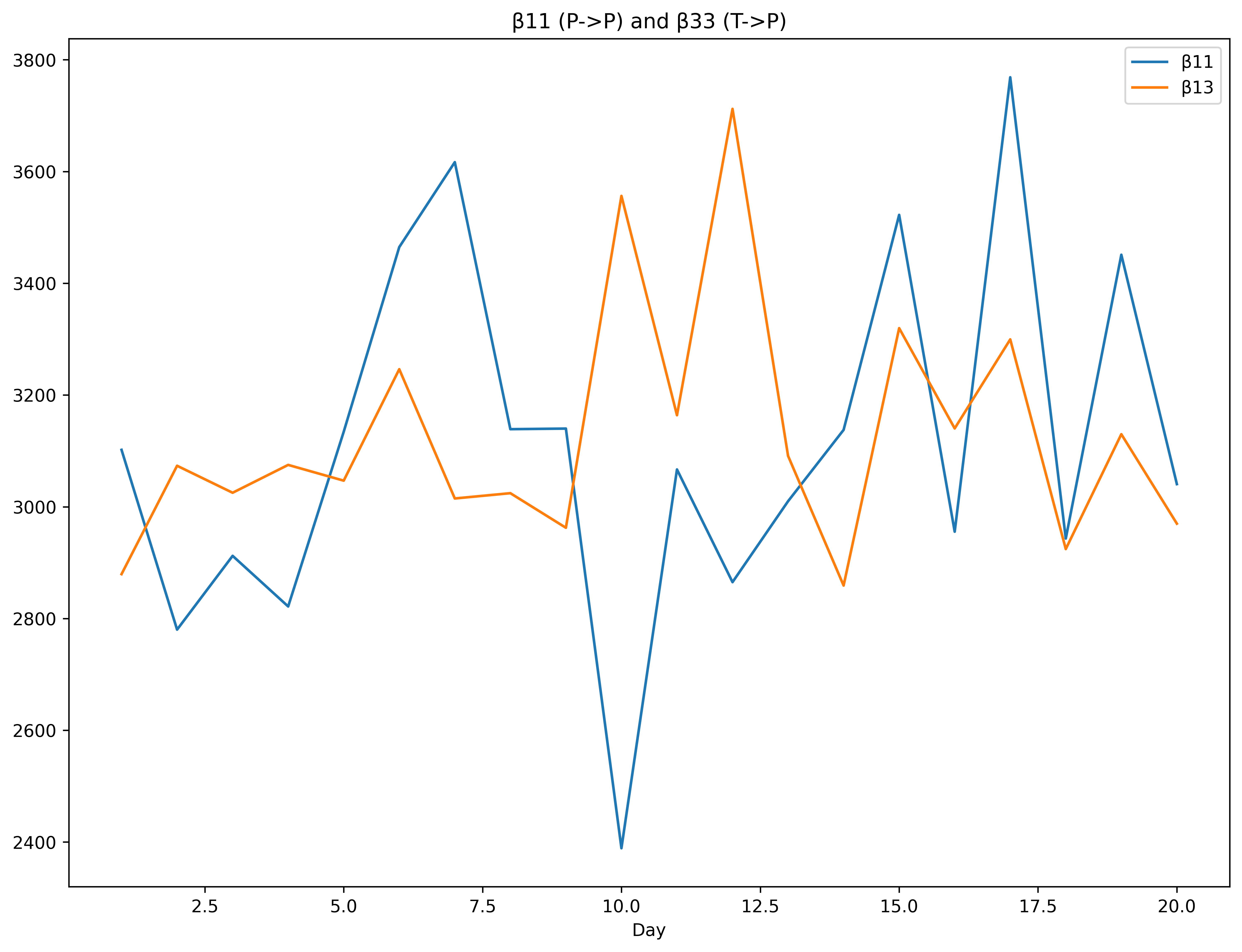
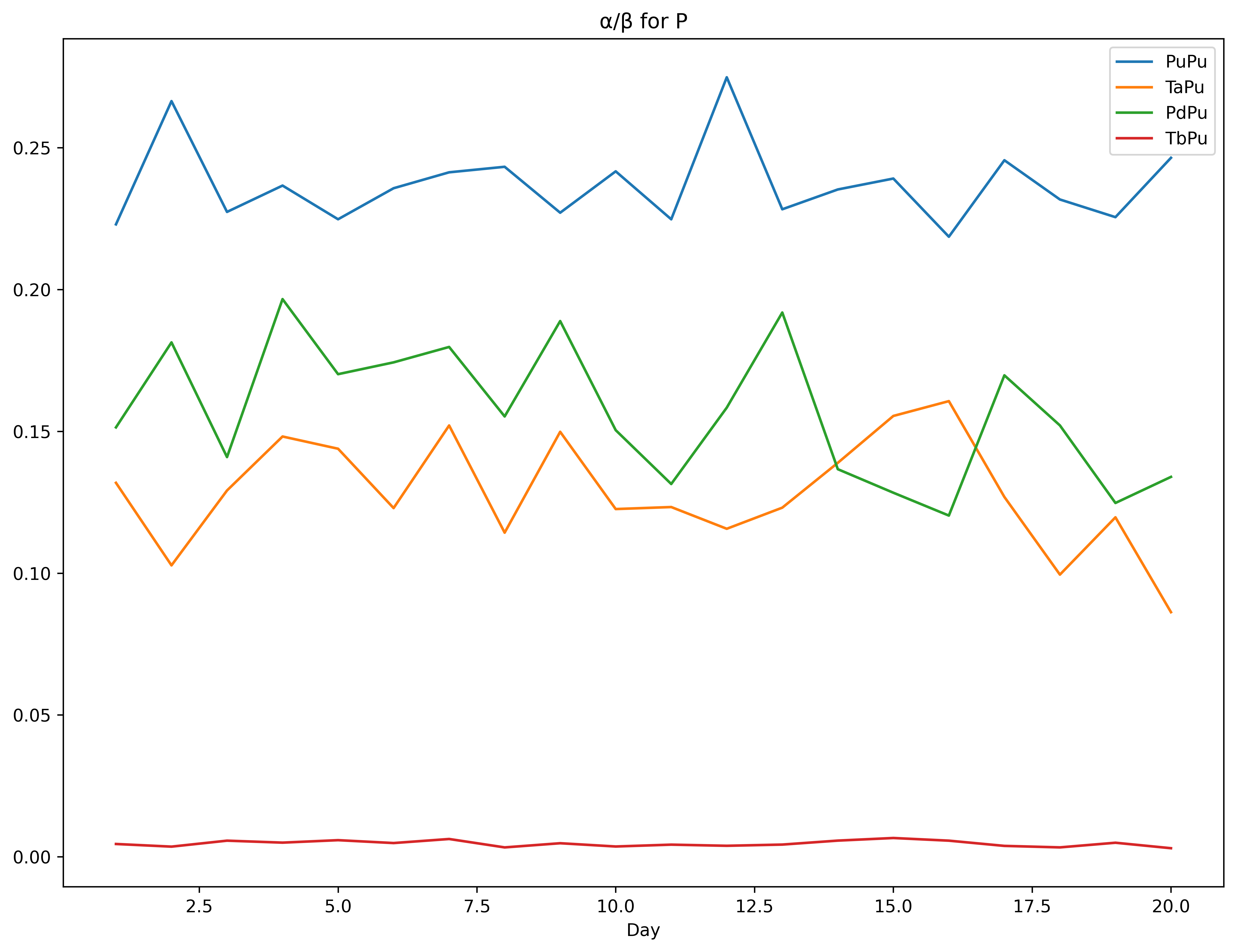
We run optimizations for the sum of (Bid+Ask) log-likelihoods where the kernel intensities are the same within diagonals: and and the kernel decays are the same within blocks ; so the total LL is optimized individually as . We also run exploratory optimizations with completely independent intensities and decays, and tested different optimizer algorithms, in order to reduce the bounds for the parameters. The code (including initial values and bounds) is at the GitHub page, together with the spreadsheet with the results of the optimization (using the Differential Evolution, Powell and L-BFGS-B methods from [scipy]; Powell was the best-performing method). The parameters for were the most unstable (charts in the Appendix).
| 4.0% | 4.0% | 14.3% | 16.1% | |
| R | 25% | 25% | 38% | 37% |
737 488 401 14.5 3113 3125 23.7% 15.7% 12.8% 0.46%
23.6 316 3.8 (median) 0.27 (median) 1122 7.8 (median) 2.1% 28.3% 48.0% 3.1%
We calculate the exogeneity ratio R between the number of exogenous events and the total number of events n for each event type i and day d as:
| (22) |
And these ratios are much higher than those found in [Bacry et al 2016], which can be explained as the reassignment of the events within the latency. Even then we find that it is reasonable to expect that a good part of the trades are exogenous (ie caused by reasons other than short-term dynamics of the order book). Most interestingly, events that change the mid-price (trades, cancels and replenishments) are (i) faster and (ii) more endogenous than trades that do not change the mid-price. Please note how the first chart of Figure 2 is similar to the first chart of Figure 7 in [Bacry et al 2016] after approximately .
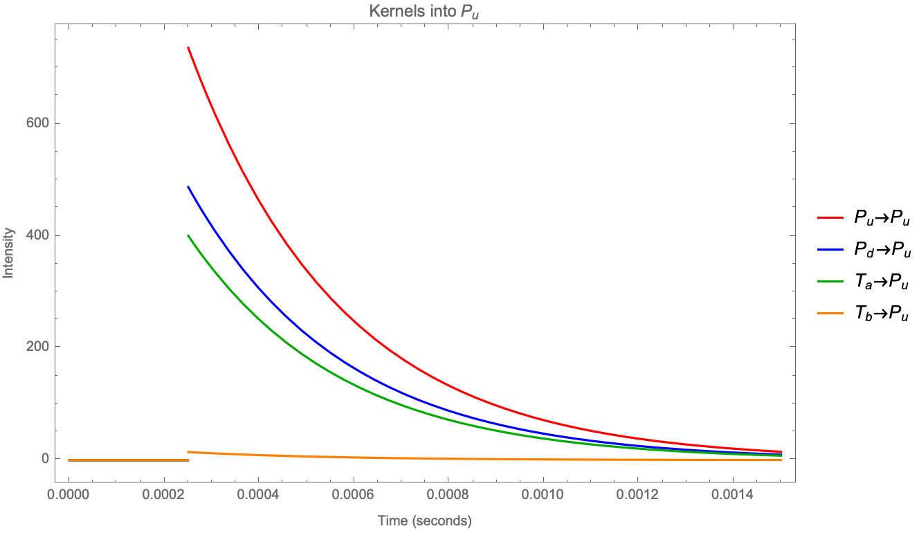
It’s not by chance that the decay on and kernels is about 3000; we can plot the first chart again but changing the x-axis to units of latency:
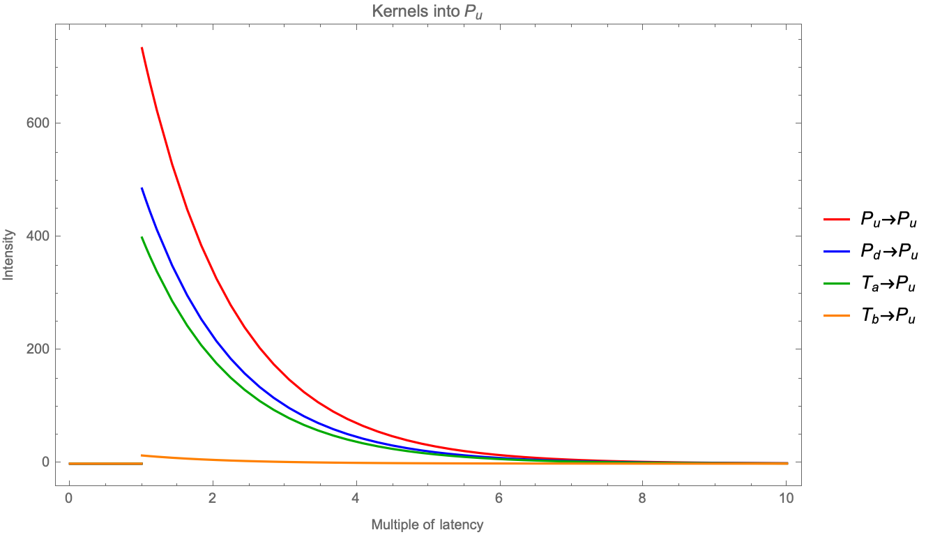
It’s expected that fast participants will act quickly on: (i) sharp imbalances by either canceling or consuming the remaining queue (ii) filling in recent gaps and that they will be able to react to the reactions as quickly as before, so the influence of the first event decays fast. We expect that Figure 3 will be found in different markets and different years (e.g. BUND futures in 2012, which had a latency of instead of ).
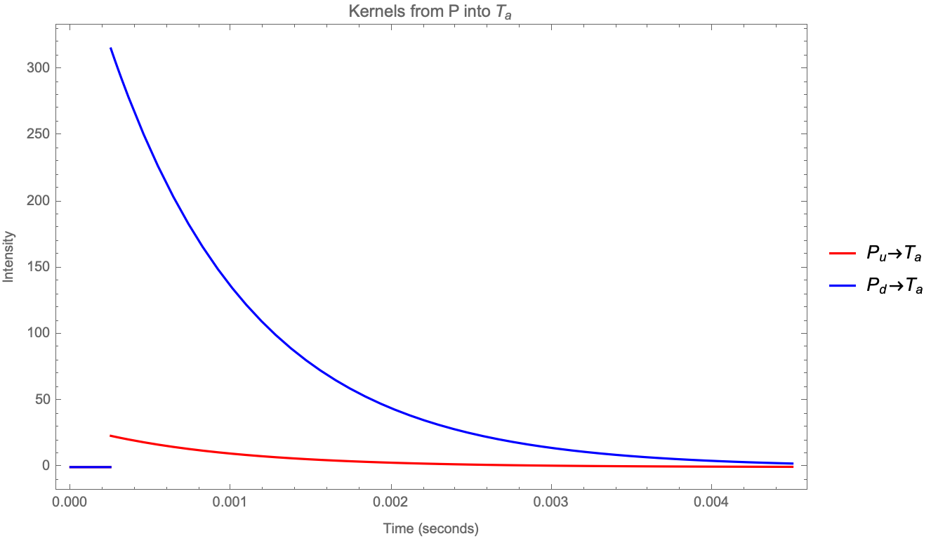
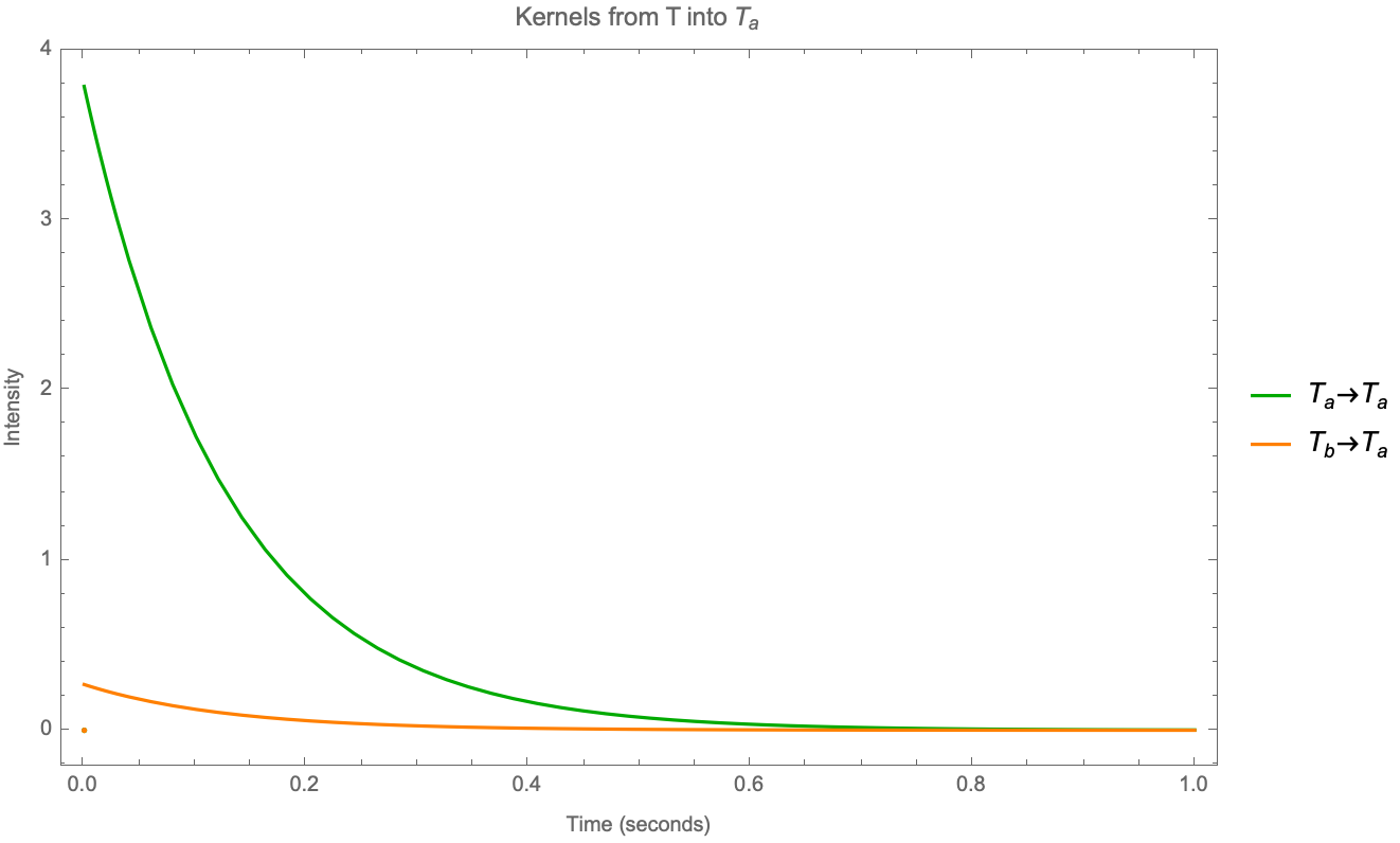
The main differences found with [Bacry et al 2016] are on the anti-diagonals. For we find that diagonals are stronger than anti-diagonals (even on a large tick asset such as the BUND future); to investigate this further a better breakdown of P into Cancels and Trades would help. For our method is not able to learn negative intensities because of the log-likelihood, but none of the values reached the lower bound; average intensity was about 2%; although a change in mid-price will make limit orders with the same sign miss the fill and become diagonals in the sub-matrix market orders would not be affected; but more importantly the speed and intensity of the kernels ensure that gaps close quickly; we think that the introduction of the latency is enough to simplify the model such that negative intensities would not be necessary.
We have not tested a Sum of Exponentials model, but it might be interesting to fix the decays for the first exponential kernel at “known” values and see what we can find.
5 Conclusions
We show (with formulas and code) how to simulate and estimate exponential kernels of Hawkes processes with a latency, and interpreted the results of applying this method to a (limited) set of BUND futures data. We show how some features of this model (the kernels and parameter symmetries) might be quite universal in markets. We can also extend this approach to two related securities that trade in different markets by using different latencies on the cross-market kernels without changing the model.
We would like to thank Mathieu Rosenbaum (CMAP) for the guidance and Sebastian Neusuess (Eurex) for the latency data.
References
- [tick] Bacry, E., Bompaire, M., Gaïffas, S. and Poulsen, S., (2017), “tick: a Python library for statistical learning, with a particular emphasis on time-dependent modeling”, available at https://arxiv.org/abs/1707.03003
- [numpy] Harris, C. P. et al (2020) “Array programming with NumPy”, Nature, 585, 357–362
- [scipy] Virtanen, P. et al (2020) “SciPy 1.0: Fundamental Algorithms for Scientific Computing in Python”, Nature Methods, 17(3), 261-272
- [Numba] Lam, S. K., Pitrou, A. and Seibert, S. (2015) “Numba: a LLVM-based Python JIT compiler”, LLVM ’15: Proceedings of the Second Workshop on the LLVM Compiler Infrastructure in HPC, Article No.: 7 Pages 1–6
- [Eurex 2017] Eurex, “Insights into trading system dynamics”, presentation
- [Abergel et al 2016] Abergel, F., Anane, M., Chakraborti, A., Jedidi, A. and Toke, I. M. (2016) “Limit Order Books”, Cambridge University Press, ISBN 978-1-107-16398-0
- [Bacry at al 2015] Bacry, E., Mastromatteo, I. and Muzy, J-F., (2015), “Hawkes processes in finance”, Market Microstructure and Liquidity 1(1)
- [Bacry et al 2016] Bacry, E., Jaisson, T. and Muzy, J. F., (2016), “Estimation of Slowly Decreasing Hawkes Kernels: Application to High Frequency Order Book Dynamics”, Quantitative Finance 16(8), 1179-1201
- [Bacry et al 2019] Bacry, E., Rambldi, M., Muzy, J. F. and Wu, P. (2019), “Queue-reactive Hawkes models for the order flow”, Working Papers hal-02409073, HAL, available at https://arxiv.org/abs/1901.08938
- [Euch et al 2016] Euch, O. E., Fukasawa, M. and Rosenbaum, M., (2018) “The microstructural foundations of leverage effect and rough volatility”, Finance and Stochastics 22, 241-280
- [Huang et al 2015] Huang, W., Lehalle, C.A. and Rosenbaum, M. (2015) “Simulating and Analyzing Order Book Data: The Queue-Reactive Model”, Journal of the American Statistical Association, 110(509):107–122
- [Kisel 2017] Kisel, R. (2017): “Quoting behavior of a market-maker under different exchange fee structures”, Master’s thesis
- [Ogata et al 1981] Ogata, Y., (1981) “On Lewis’ simulation method for point processes”, IEEE Transactions on Information Theory 27(1), 23-31
- [Toke 2011] Toke, I. M., (2011), “An Introduction to Hawkes Processes with Applications to Finance”, BNP Paribas Chair Meeting, available at http://lamp.ecp.fr/MAS/fiQuant/ioane_files/HawkesCourseSlides.pdf
Appendix
Appendix A Appendix
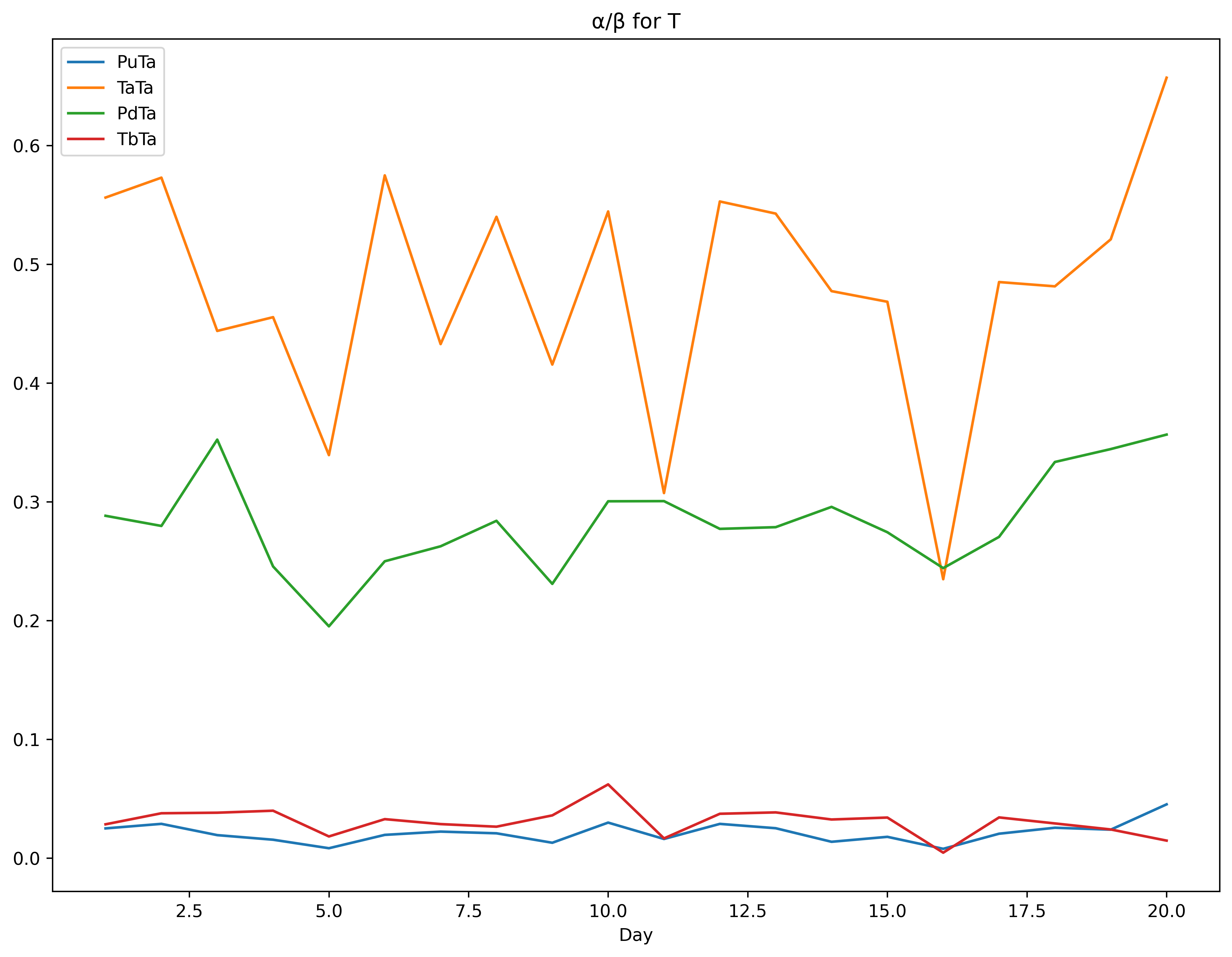
The charts and tables for the daily estimates are below. The only real worry is the instability of the parameters of the kernels, although the intensities are stable. The upper bound for was hit on day 16.
| Day | |||
|---|---|---|---|
| 1 | 2.73 | 0.14 | 4.91 |
| 2 | 2.80 | 0.18 | 4.88 |
| 3 | 3.81 | 0.33 | 8.57 |
| 4 | 7.12 | 0.62 | 15.64 |
| 5 | 36.12 | 1.94 | 106.44 |
| 6 | 2.96 | 0.17 | 5.15 |
| 7 | 4.68 | 0.31 | 10.81 |
| 8 | 4.19 | 0.21 | 7.75 |
| 9 | 7.78 | 0.67 | 18.73 |
| 10 | 2.55 | 0.29 | 4.68 |
| 11 | 22.68 | 1.22 | 73.79 |
| 12 | 2.28 | 0.15 | 4.13 |
| 13 | 3.33 | 0.24 | 6.14 |
| 14 | 4.04 | 0.27 | 8.46 |
| 15 | 4.75 | 0.35 | 10.15 |
| 16 | 117.41 | 2.28 | 500.00 |
| 17 | 3.85 | 0.27 | 7.93 |
| 18 | 3.63 | 0.22 | 7.54 |
| 19 | 3.24 | 0.15 | 6.22 |
| 20 | 1.76 | 0.04 | 2.68 |