Exponential quadrature rules without order reduction
Abstract
In this paper a technique is suggested to integrate linear initial boundary value problems with exponential quadrature rules in such a way that the order in time is as high as possible. A thorough error analysis is given for both the classical approach of integrating the problem firstly in space and then in time and of doing it in the reverse order in a suitable manner. Time-dependent boundary conditions are considered with both approaches and full discretization formulas are given to implement the methods once the quadrature nodes have been chosen for the time integration and a particular (although very general) scheme is selected for the space discretization. Numerical experiments are shown which corroborate that, for example, with the suggested technique, order is obtained when choosing the nodes of Gaussian quadrature rule.
1 Introduction
Due to the recent development and improvement of Krylov methods [7, 11], exponential quadrature rules have become a valuable tool to integrate linear initial value partial differential problems [9]. This is because of the fact that the linear and stiff part of the problem can be ‘exactly’ integrated in an efficient way through exponential operators. Moreover, when the source term is nontrivial, a variations-of-constants formula and the interpolation of that source term in several nodes leads to the appearance of some -operators, to which Krylov techniques can also be applied.
However, in the literature [9], these methods have always been applied and analysed either on the initial value problem or on the initial boundary value one with vanishing or periodic boundary conditions. More precisely, when the linear and stiff operator is the infinitesimal generator of a strongly continuous semigroup in a certain Banach space. In such a case, it has been proved [9] that the exponential quadrature rule converges with global order if is the number of nodes being used for the interpolation of the source term.
There are no results concerning specifically how to deal with these methods when integrating the most common non-vanishing and time-dependent boundary conditions case. The only related reference is that of Lawson quadrature rules [3, 4, 10] which differ from these methods in the fact that, not only the source term is interpolated, but all the integrand which turns up in the variations-of-constants formula. In such a way, with the latter methods, -operators (with ) do not turn up. Only exponential functions (those corresponding to ) are present. In [3] a thorough error analysis is given which studies the strong order reduction which turns up with Lawson methods even in the vanishing boundary conditions case unless some even more artificial additional vanishing boundary conditions are satisfied. Nevertheless, in [4], a technique is suggested to avoid that order reduction under homogeneous boundary conditions and to even tackle the time-dependent boundary case without order reduction. Moreover, the analysis there also includes the error coming from the space discretization.
The aim of this paper is to generalize that technique to the most common quadrature rules which are used in the literature and which also use -operators. Besides, we also include the error coming from the space discretization not only when avoiding order reduction but also with the classical approach. We will see that, with the technique which is suggested in this paper, we manage to get the order of the classical quadrature interpolatory rule, which implies that, by choosing the nodes carefully, we can manage to get even order in time.
The paper is structured as follows. Section 2 gives some preliminaries on the abstract framework in Banach spaces which is used for the time integration of the problem, on the definition of the exponential quadrature rules and on the general hypotheses which are used for the abstract space discretization. Then, Section 3 describes and makes a thorough error analysis of the classical method of lines, which integrates the problem firstly in space and then in time. Both vanishing and nonvanishing boundary conditions are considered there and several different results are obtained depending on the specific accuracy of the quadrature rule and on whether a parabolic assumption is satisfied. After that, the technique which is suggested in the paper to improve the order of accuracy in time is well described in Section 4. It consists of discretizing firstly in time with suitable boundary conditions and then in space. Therefore, the analysis is firstly performed on the local error of the time semidiscretization and then on the local and global error of the full scheme (27),(32),(33). Finally, Section 5 shows some numerical results which corroborate the theoretical results of the previous sections.
2 Preliminaries
As in [4], we consider the linear abstract initial boundary value problem in the complex Banach space
| (4) |
where is a dense subspace of and the linear operators and satisfy the following assumptions:
-
(A1)
The boundary operator is onto, where is another Banach space.
-
(A2)
Ker() is dense in and , the restriction of to Ker(), is the infinitesimal generator of a - semigroup in , which type is denoted by , and we assume that it is negative.
-
(A3)
If satisfies and , then the steady state problem
possesses a unique solution denoted by . Moreover, the linear operator satisfies
where the constant holds for any such that .
As precisely stated in [4, 12], with these assumptions, problem (4) is well-posed in sense. Moreover, as is negative, the semigroup decays exponentially when and the operator is invertible.
We also remind that, because of hypothesis (A2), are bounded operators for , where are the standard functions which are used in exponential methods [9]:
| (5) |
It is well-known that they can be calculated in a recursive way through the formula
| (6) |
and that these functions are bounded on the complex plane when .
We also assume that the solution of (4) satisfies that, for a natural number ,
| (7) |
When is a differential space operator, this assumption implies that the time derivatives of the solution are regular in space, but without imposing any restriction on the boundary. Because of Theorem 3.1 in [1], this assumption is satisfied when the data , and are regular and satisfy certain natural compatibility conditions at the boundary. Moreover, as from (4),
| (8) |
the following crucial boundary values
can be calculated from the given data in problem (4).
We will center on exponential quadrature rules [9] to time integrate (4). When applied to a finite-dimensional linear problem like
| (9) |
where is a matrix, these rules correspond to interpolating in nodes in the integral in the equality
| (10) |
which is satisfied by the solutions of (9) when . This yields
with weights
where are the Lagrange interpolation polynomials corresponding to the nodes . We will define the values in such a way that
| (11) |
From this,
for the functions in (5), and the final formula for the integration of (9) is
| (12) |
We will consider an abstract spatial discretization which satisfies the same hypotheses as in [4] (Section 4.1) and which includes a big range of techniques. In such a way, for each parameter in a sequence such that , is a finite dimensional space which approximates when and the elements in are approximated in a subspace . The norm in is denoted by . The operator is then approximated by , by and the solution of the elliptic problem
is approximated by , where is called the elliptic projection, discretizes the boundary values and the following is satisfied:
| (13) |
for a projection operator . We will also use and we remind part of hypothesis (H3) in [4], which states that, for a subspace of with norm , whenever ,
| (14) |
for decreasing with and, therefore, this gives a bound for the error in the space discretization of operator .
Moreover, we will assume that this additional hypothesis is satisfied:
-
(HS)
is bounded independently of for small enough . Considering (13), this in fact corresponds to a discrete maximum principle, which would be simulating the continuous maximum principle which is satisfied because of (A3) when .
3 Classical approach: Discretizing firstly in space and then in time
When considering vanishing boundary conditions in (4) (which has been classically done in the literature with exponential methods [9]), discretizing first in space and then in time leads to the following semidiscrete problem in :
When integrating this problem with an exponential quadrature rule which is based on nodes (12), the following scheme arises:
| (15) |
Denoting by to where is the result of applying (15) from instead of ; and to the following result follows:
Theorem 1.
Whenever in (4), and ,
-
(i)
,
-
(ii)
,
-
(iii)
.
where the constants in Landau notation are independent of and .
Proof.
(i) comes from the fact that the difference between and its interpolant in those nodes is . More explicitly, by using (10) and the definition of ,
| (16) |
Now, taking into account hypotheses (H1)-(H2) in [4], and are bounded with , and the result follows.
Then, (ii) is deduced from the classical argument for the global error once the local error is bounded. Finally, (iii) comes from (ii) and the decomposition
by noticing that, for the first term, as , it happens that
Then, because of (14),
We also have this finer result, which implies global order under more restrictive hypotheses.
Theorem 2.
Let us assume that in (4), belongs to , to , the interpolatory quadrature rule which is based on integrates exactly polynomials of degree less than or equal to and this bound holds
| (17) |
Then,
-
(i)
,
-
(ii)
,
-
(iii)
.
where the constants in Landau notation are independent of and .
Proof.
To prove (i), it suffices to consider the following formula for the interpolation error which is valid when :
Then, substituting in (16) and multiplying by ,
where we have used (6), (H1)-(H2) in [4] and the fact that the integral in brackets vanishes because the interpolatory quadrature rule is exact for polynomials of degree .
Remark 3.
Notice that, when is symmetric with negative eigenvalues and is the discrete -norm, coincides with its spectral radius. As, for each eigenvalue ,
and this is bounded in the negative real axis, (17) follows. In fact, this bound has been proved in [8] for analytic semigroups covering the case in which (4) corresponds to parabolic problems. Therefore it seems natural that it is also satisfied by a suitable space discretization.
On the other hand, when in (4), the semidiscretized problem which arises is
| (20) |
In a similar way as before, the local error would be given by
| (21) | |||||
Again, when and , the error of interpolation will be . However, although and are bounded [4], is not bounded any more. That is why we state the following result which bounds in fact by using (HS) and which proof for the global error is the same as in Theorem 2.
Theorem 4.
Remark 5.
In any case, we want to remark in this section that accuracy has been lost with respect to the vanishing boundary conditions case since order reduction turns up at least for the local error and, in many cases, also for the global error.
4 Suggested approach: Discretizing firstly in time and then in space
In this section, we directly tackle the nonvanishing boundary conditions case by discretizing in a suitable way firstly in time and then in space. We will see that we manage to get at least the same order as with the classical approach when vanishing boundary conditions are present, but even a much higher order some times.
Let us suggest how to apply the exponential quadrature rule (12) directly to (4). When , in (12) is directly substituted by and there is no problem because and have perfect sense over . However, it has no sense to do that when because is not any more. For Lawson methods, for which just exponential functions appear, instead of , it was suggested in [4] to consider as the solution of
| (22) |
whenever . In such a way, if ,
| (23) |
which resembles the formal analytic expansion of the exponential of applied over . In this manuscript then, whenever , for , instead of , we suggest to consider the following functions :
| (24) |
This resembles the formal analytic expansion of when evaluated at and applied over . (Notice that, for , this would correspond to (23) changing by . As the functions are multiplied by in (12), we need one less term in this expansion.)
Therefore, imitating (12), we suggest to consider as continuous numerical approximation from the previous ,
| (25) | |||||
It is not practical to discretize directly this formula in space since numerical differentiation is a badly-posed problem. However, if we seek a differential equation which the functions (24) satisfy and apply a numerical integrator to it, there should be no problems. For that, let us first consider the following lemma.
Lemma 6.
For ,
Proof.
It suffices to differentiate considering (5),
From here, the next result follows:
Lemma 7.
The function in (24) satisfies the following initial boundary value problem:
| (26) |
Proof.
Notice that, using Lemma 6,
On the other hand,
where the change has been used in the second line for the first sum. Therefore, the lemma is proved taking also into account that .
With Lawson methods [4], starting from a previous approximation to and discretizing (22) in space with in led to a term like
| (27) | |||||
which is the approximation which corresponds to the first term in (12).
For the rest of the terms in (12), we suggest to discretize (26) in space with . In such a way, the following system turns up:
where
This can be rewritten as
| (28) |
With the same arguments as in Lemma 6, is the solution of
Therefore, in order to solve (28), we are interested in finding
| (29) |
which is the solution of
| (30) |
Now, using the first line of (26) for the boundary with ,
the fact that
and that the boundary of the second term vanishes, it follows that
Using this in (30),
| (31) | |||||
Therefore, using (29),
| (32) | |||||
and the overall exponential quadrature rule would be given by
| (33) |
4.1 Time semidiscretization error
Let us first study just the error after time discretization. The local truncation error is well-known to be given by , where is given by expression (25) substituting by .
Let us first consider the following general result, which will allow to conclude more particular results depending on the choice of the values .
Lemma 8.
Under the assumptions of regularity (7), the local truncation error satisfies
Proof.
Notice that can be written as
where the Taylor expansion of has been used as well as changes of subindexes.
Proof.
Theorem 10.
Proof.
With the same argument as in the previous lemma, all the terms in brackets in the expression of in Lemma 8 vanish for . Then, for , the term in parenthesis vanishes for the same reason when . It just suffices to see what happens when and . But, as the quadrature rule which is based on is assumed to be exact for the polynomial ,
From this, the result also directly follows.
We now state the following much more general result:
Theorem 11.
Proof.
It suffices to notice that, for , with , due to the hypothesis,
Now, the left-hand side term above can inductively be proved to be
and the right-hand side can be written as
Then, using Lemma 8, the result directly follows.
From this, the following interesting results are achieved:
Corollary 12.
Remark 13.
Due to the fact that the last node of one step is the first of the following, the nodes corresponding to the Gaussian-Lobatto quadrature rule have the advantage that just (instead of ) terms of the form must be calculated in (33).
4.2 Full discretization error
4.2.1 Local error
To define the local error after full discretization, we consider
where
-
(i)
is the solution of
with .
-
(ii)
is the solution of (28) substituting by . More precisely,
(34)
Then, we define and the following is satisfied.
Theorem 14.
Proof.
Because of definition,
| (36) | |||||
where and are those defined in Section 4.1. The fact that (35) is satisfied implies that belongs to and therefore . Moreover, and, using the same proof as that of Theorem 11 in [4],
| (37) |
On the other hand,
| (38) |
where corresponds to (23) with and corresponds to (24) with . In the same way as in the proof of Theorem 4.4 in [4],
| (39) |
Moreover, using Lemma 7,
and making the difference with (34), it follows that
where we have used that
because of Lemma 7. Now, due to the same lemma and (34), , and therefore
| (40) | |||||
Here we have used that because of (35) and Lemma 3.3 in [4]. Finally, gathering (36)–(40), the result follows.
4.2.2 Global error
We now study the global error, which we define as .
Theorem 15.
Proof.
As in the proof of Theorem 4.5 in [4],
| (41) | |||||
The difference is that now, using (33),
As in [4],
As for , making the difference between (34) and (28),
Considering then an analogue of Lemma 6 substituting by and taking into account that (6),
Therefore,
This implies that
which, together with the first line of (33), (14), (41) and Theorem 14, implies the result.
5 Numerical experiments
In this section we will show some numerical experiments which corroborate the previous results. For that, we have considered parabolic problems with homogeneous and non-homogeneous Dirichlet boundary conditions for which for a certain spatial domain and . The fact that these problems can be well fitted under the theory of abstract IBVPs is well justified in [4, 13]. Moreover, other types of boundary conditions can also be considered although we restrict here to Dirichlet boundary conditions just for the sake of brevity.
As for the space discretization, we have considered here both the standard symmetric 2nd-order finite differences and collocation spectral methods in dimension. For the former, it was already well justified in [4] that the hypotheses which are required on the space discretization are satisfied, at least for the discrete -norm, and . Besides, a discrete maximum principle (hypothesis (HS)) is well-known to apply [14]. With the collocation spectral methods, those hypotheses are also valid with the discrete -norm associated to the corresponding Gaussian-Lobatto quadrature rule (), and [2, 6], where is the number of collocation nodes, which is clearly inversely proportional to the diameter space grid . In such a way, the more regular the functions are, the quicker the numerical solution of the elliptic problems converges to the exact solution.
Besides, although in the collocation case the matrix is not symmetric any more, Remarks 3 and 5 still apply. Notice that, for every matrix of dimension ,
| (42) |
where denotes the diagonal matrix which contains the square root of the coefficients of the quadrature rule corresponding to the interior Gauss-Lobatto nodes . (We will denote them by .) Because of this, when is symmetric, . The fact that is symmetric comes from the following: Notice that where are the Lagrange polynomials associated to the interior Gauss-Lobatto nodes and those at the boundary. As vanish at the boundary, integrating by parts, for every ,
As the integrand in the left-hand side is a polynomial of degree , the corresponding Gaussian-Lobatto quadrature rule integrates it exactly. Therefore,
where, for the last equality, the role of and has been interchanged. From this, and using (42) again,
As is symmetric, the matrix inside is also symmetric and therefore
Secondly, the eigenvalues of are negative. This is due to the following: For every polynomial which vanishes at the boundary such that ,
Considering and using the Gauss-Lobatto quadrature rule and the definition of Lagrange polynomials,
This can be rewritten as for every vector , or equivalently, , which implies that has negative eigenvalues and so has .
For both types of discretizations which have been considered here, and therefore formulas (27) and (32) simplify a little bit. However, other possible discretizations (as those considered in [4]) are also possible, for which that simplification cannot be made.
In all cases, we have considered the one-dimensional problem
| (43) |
with the corresponding functions , , and which make that or are solutions of the problem. These functions satisfy regularity hypotheses (7) and (35) for any natural number .
5.1 Trapezoidal rule
We begin by considering the trapezoidal rule in time and the second-order finite differences in space. We have considered so that the error in space is negligible. The trapezoidal rule corresponds to but is just exact for polynomials of degree . Therefore, one of the hypothesis of Theorem 2 is not satisfied and we can just apply Theorem 1 when discretizating firstly in space and then in time with the solution which satisfies . That theorem states that, with respect to the time stepsize , the local and global error should show orders and respectively and we can check that really happens in Table 1. For the same problem, but applying the technique which is suggested in this paper (33) with , Theorems 9, 14 and 15 state that also the local and global error should show orders and respectively and that is what we can in fact observe in the same table. We can see that, although the local order is a bit more clear with the suggested technique, the size of the errors is slightly bigger with the suggested approach. Therefore, it seems that, in this particular problem, the error constants are bigger with the suggested technique and it is not worth the additional cost of calculating terms which contain and .
The comparison is more advantageous for the suggested technique when the solution is such that it does not vanish at the boundary. Then, Theorem 4 and Remark 5 state that the local and global error should show order with the classical approach and that can be checked in Table 2. However, with the suggested strategy, as with the vanishing boundary conditions case, the theorems in this paper prove local order and global order , which can again be checked in the same table. The fact that we manage to increase the order in the local error makes that the global errors, although always of order , are smaller with the suggested technique than with the classical approach. Nevertheless, the comparison between both techniques will be more beneficial for the technique which is suggested in the paper when the classical (non-exponential) order of the quadrature rule increases.
| Classical approach | Suggested approach | |||||||
| k | Loc. err. | ord. | Glob. err. | ord. | Loc. err. | ord. | Glob. err. | ord. |
| 1/10 | 8.0170e-5 | 5.5395e-5 | 1.5334e-4 | 9.8091e-5 | ||||
| 1/20 | 1.2961e-5 | 2.6 | 1.3953e-5 | 2.0 | 1.9139e-5 | 3.0 | 1.8575e-5 | 2.4 |
| 1/40 | 1.8644e-6 | 2.8 | 3.4952e-6 | 2.0 | 2.3902e-6 | 3.0 | 4.0262e-6 | 2.2 |
| 1/80 | 2.5316e-7 | 2.9 | 8.7426e-7 | 2.0 | 2.9862e-7 | 3.0 | 9.3773e-7 | 2.1 |
| 1/160 | 3.3354e-8 | 2.9 | 2.1860e-7 | 2.0 | 3.7318e-8 | 3.0 | 2.2635e-7 | 2.0 |
| 1/320 | 4.3171e-9 | 3.0 | 5.4651e-8 | 2.0 | 4.6641e-9 | 3.0 | 5.5610e-8 | 2.0 |
| Classical approach | Suggested approach | |||||||
| k | Loc. err. | ord. | Glob. err. | ord. | Loc. err. | ord. | Glob. err. | ord. |
| 1/10 | 7.4531e-4 | 4.8108e-4 | 2.0144e-4 | 1.3742e-4 | ||||
| 1/20 | 1.5446e-4 | 2.3 | 1.2476e-4 | 2.0 | 2.8775e-5 | 2.8 | 3.0165e-5 | 2.2 |
| 1/40 | 3.3863e-5 | 2.2 | 3.2074e-5 | 2.0 | 3.9084e-6 | 2.9 | 7.0453e-6 | 2.1 |
| 1/80 | 7.3906e-6 | 2.2 | 8.1809e-6 | 2.0 | 5.1475e-7 | 2.9 | 1.6979e-6 | 2.0 |
| 1/160 | 1.5848e-6 | 2.2 | 2.0770e-6 | 2.0 | 6.6122e-8 | 3.0 | 4.1324e-7 | 2.0 |
| 1/320 | 3.3666e-7 | 2.2 | 5.2777e-7 | 2.0 | 8.1531e-9 | 3.0 | 9.8459e-8 | 2.1 |
5.2 Simpson rule
In this subsection we consider Simpson rule in time and a collocation spectral method in space with nodes so that the error in space is negligible. As Simpson rule corresponds to and the interpolatory quadrature rule which is based in those nodes is exact for polynomials of degree , we can take in Theorem 10 and achieve orders and for the local and global error respectively with the technique suggested here. However, with the classical approach, at least in the common case that , Theorem 4 and Remark 5 give just order for the local and global error. These results can be checked in Table 3. Moreover, the size of the global error, even for the bigger timestepsizes is smaller with the suggested technique.
We also want to remark here that the trapezoidal and Simpson rules correspond to Gauss-Lobatto quadrature rules with and respectively and therefore Corollary 12 (ii) and Remark 13 apply.
| Classical approach | Suggested approach | |||||||
| k | Loc. err. | ord. | Glob. err. | ord. | Loc. err. | ord. | Glob. err. | ord. |
| 1/2 | 8.0718e-4 | 4.9507e-4 | 2.7496e-4 | 1.6821e-4 | ||||
| 1/4 | 8.3265e-5 | 3.3 | 4.2862e-5 | 3.5 | 8.5778e-6 | 5.0 | 4.4156e-6 | 5.2 |
| 1/8 | 8.6214e-6 | 3.3 | 4.0561e-6 | 3.4 | 2.6785e-7 | 5.0 | 1.5345e-7 | 4.8 |
| 1/16 | 1.0500e-6 | 3.0 | 4.4103e-7 | 3.2 | 8.3681e-9 | 5.0 | 6.7803e-9 | 4.5 |
| 1/32 | 1.1622e-7 | 3.2 | 4.6864e-8 | 3.2 | 2.6148e-10 | 5.0 | 3.5342e-10 | 4.3 |
| 1/64 | 1.2378e-8 | 3.2 | 4.9423e-9 | 3.2 | 8.1711e-12 | 5.0 | 2.0189e-11 | 4.1 |
5.3 Gaussian rules
In order to achieve the highest accuracy given a certain number of nodes, we consider in this subsection Gaussian quadrature rules. More precisely, those corresponding to . As space discretization, we have considered again the same spectral collocation method of the previous subsection. Following Corollary 12 (i) and Theorem 14, even for non-vanishing boundary conditions, taking in (27) and (32) the local error in time should show order and the global error, using Theorem 15, order . This should be compared with the order which is proved for the classical approach when in Theorem 2 and the order for the local and global error when , which comes from Theorem 4 and Remark 5. In Tables 4 and 5 we see the results which correspond to and respectively for the vanishing boundary conditions case. Although for there is not an improvement on the global order for the suggested technique, the errors are a bit smaller. Of course the benefits are more evident with . For the non-vanishing boundary conditions case, Tables 6,7,8 and 9 show the results which correspond to and respectively. When avoiding order reduction, the results are much better than with the classical approach. Not only the order is bigger but also the size of the errors is smaller from the very beginning. We notice that the global order is even a bit better than expected for the first values of .
| Classical approach | Suggested approach | |||||||
| k | Loc. err. | ord. | Glob. err. | ord. | Loc. err. | ord. | Glob. err. | ord. |
| 1/4 | 8.2639e-3 | 4.3743e-3 | 4.9483e-3 | 2.5685e-3 | ||||
| 1/8 | 1.8874e-3 | 2.1 | 1.1548e-3 | 1.9 | 6.4427e-4 | 2.9 | 3.7820e-4 | 2.8 |
| 1/16 | 3.6716e-4 | 2.4 | 2.9791e-4 | 2.0 | 8.2199e-5 | 3.0 | 6.9202e-5 | 2.4 |
| 1/32 | 7.6916e-5 | 2.2 | 7.6389e-5 | 2.0 | 1.0381e-5 | 3.0 | 1.4677e-5 | 2.2 |
| 1/64 | 1.6803e-5 | 2.2 | 1.9445e-5 | 2.0 | 1.3043e-6 | 3.0 | 3.3796e-6 | 2.1 |
| 1/128 | 3.6111e-6 | 2.2 | 4.9232e-6 | 2.0 | 1.6345e-7 | 3.0 | 8.1115e-7 | 2.1 |
| Classical approach | Suggested approach | |||||||
| k | Loc. err. | ord. | Glob. err. | ord. | Loc. err. | ord. | Glob. err. | ord. |
| 1/2 | 8.9292e-4 | 5.4788e-4 | 8.2591e-5 | 5.0573e-5 | ||||
| 1/4 | 8.6746e-5 | 3.4 | 4.5296e-5 | 3.6 | 2.8465e-6 | 4.9 | 1.4782e-6 | 5.1 |
| 1/8 | 8.1186e-6 | 3.4 | 3.9933e-6 | 3.5 | 9.3457e-8 | 4.9 | 5.4928e-8 | 4.7 |
| 1/16 | 1.0237e-6 | 3.0 | 4.3449e-7 | 3.2 | 2.9938e-9 | 5.0 | 2.5254e-9 | 4.4 |
| 1/32 | 1.1415e-7 | 3.2 | 4.6048e-8 | 3.2 | 9.4726e-11 | 5.0 | 1.3424e-10 | 4.2 |
| 1/64 | 1.2112e-8 | 3.2 | 4.8418e-9 | 3.2 | 2.9786e-12 | 5.0 | 7.7190e-12 | 4.1 |
| Classical approach | Suggested approach | |||||||
| k | Loc. err. | ord. | Glob. err. | ord. | Loc. err. | ord. | Glob. err. | ord. |
| 1/8 | 6.6985e-2 | 2.8814e-2 | 1.5650e-3 | 8.6254e-4 | ||||
| 1/16 | 3.0444e-2 | 1.1 | 1.2167e-2 | 1.2 | 1.8673e-4 | 3.1 | 1.4048e-4 | 2.6 |
| 1/32 | 1.3218e-2 | 1.2 | 5.1128e-3 | 1.2 | 2.2356e-5 | 3.1 | 2.7661e-5 | 2.3 |
| 1/64 | 5.6269e-3 | 1.2 | 2.1472e-3 | 1.2 | 2.6947e-6 | 3.1 | 6.1319e-6 | 2.2 |
| 1/128 | 2.3791e-3 | 1.2 | 9.0138e-4 | 1.2 | 3.2718e-7 | 3.0 | 1.4450e-6 | 2.1 |
| 1/256 | 1.0015e-3 | 1.2 | 3.7813e-4 | 1.2 | 3.9993e-8 | 3.0 | 3.5085e-7 | 2.0 |
| Classical approach | Suggested approach | |||||||
| k | Loc. err. | ord. | Glob. err. | ord. | Loc. err. | ord. | Glob. err. | ord. |
| 1/2 | 1.9328e-2 | 1.1743e-2 | 7.9408e-4 | 4.8503e-4 | ||||
| 1/4 | 4.8715e-3 | 2.0 | 2.3068e-3 | 2.3 | 2.2565e-5 | 5.1 | 1.1356e-5 | 5.4 |
| 1/8 | 1.1460e-3 | 2.1 | 4.7811e-4 | 2.3 | 6.3799e-7 | 5.1 | 3.3399e-7 | 5.1 |
| 1/16 | 2.5199e-4 | 2.2 | 9.8750e-5 | 2.3 | 1.8167e-8 | 5.1 | 1.2423ee-8 | 4.7 |
| 1/32 | 5.4061e-5 | 2.2 | 2.0543e-5 | 2.3 | 5.2222e-10 | 5.1 | 5.7608e-10 | 4.4 |
| 1/64 | 1.1476e-5 | 2.2 | 4.2930e-6 | 2.3 | 1.4918e-11 | 5.1 | 2.9580e-11 | 4.3 |
| Classical approach | Suggested approach | |||||||
| k | Loc. err. | ord. | Glob. err. | ord. | Loc. err. | ord. | Glob. err. | ord. |
| 1/2 | 8.4732e-4 | 5.1405e-4 | 3.0107e-6 | 1.8363e-6 | ||||
| 1/4 | 1.0734e-4 | 3.0 | 5.0710e-5 | 3.3 | 2.0423e-8 | 7.2 | 1.0082e-8 | 7.5 |
| 1/8 | 1.2260 e-5 | 3.1 | 5.1107e-6 | 3.3 | 1.3840e-10 | 7.2 | 6.6752e-11 | 7.2 |
| 1/16 | 1.3379e-6 | 3.2 | 5.2398e-7 | 3.3 | 9.4087e-13 | 7.2 | 5.3198e-13 | 7.0 |
| 1/32 | 1.4335e-7 | 3.2 | 5.4413e-8 | 3.3 | 6.4275e-15 | 7.2 | 5.3534e-15 | 6.6 |
| 1/64 | 1.5182e-8 | 3.2 | 5.6735e-9 | 3.3 | 4.4259e-17 | 7.2 | 6.6517e-17 | 6.3 |
| Classical approach | Suggested approach | |||||||
| k | Loc. err. | ord. | Glob. err. | ord. | Loc. err. | ord. | Glob. err. | ord. |
| 1/2 | 2.7746e-5 | 1.6829e-5 | 8.1253e-9 | 4.9495e-9 | ||||
| 1/4 | 1.7137e-6 | 4.0 | 8.0951e-7 | 4.4 | 1.3502e-11 | 9.2 | 6.5604e-12 | 9.6 |
| 1/8 | 9.6826e-8 | 4.1 | 4.0363e-8 | 4.3 | 2.2443e-14 | 9.2 | 1.0107e-14 | 9.3 |
| 1/16 | 5.2833e-9 | 4.2 | 2.0690e-9 | 4.3 | 3.7267e-17 | 9.2 | 1.7380e-17 | 9.2 |
| 1/32 | 2.8240e-10 | 4.2 | 1.0719e-10 | 4.3 | 6.2266e-20 | 9.2 | 3.5644e-20 | 8.9 |
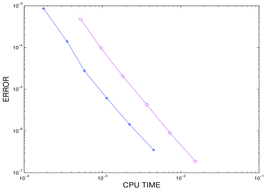
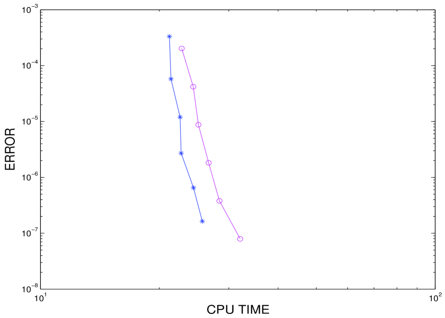
Finally, although it is not an aim of this paper, in order to compare roughly the results in terms of computational cost, let us concentrate on Gaussian quadrature rules of the same order when integrating a non-vanishing boundary value problem. When considering nodes with the classical approach, evaluations of the source term must be made at each step and the operators are needed, which will be multiplied by vectors with all its components varying in principle at each step. However, with the suggested technique and nodes, just evaluations of the source term must be made although operators are needed. Nevertheless, from these , just the first of them are multiplied by vectors which change independently in all their components at each step. The other are multiplied by vectors which just contain information on the boundary. Therefore, with finite differences many components vanish and, with Gauss-Lobatto spectral methods, those vectors are just a time-dependent linear combination of two vectors which do not change with time. With Gauss-Lobatto methods, as is not sparse but its size its moderate, we have calculated once and for all at the very beginning , , and the two necessary vectors derived from , . Then, in (33) the terms containing the former at each step require operations while the terms containing the latter just require operations. With finite differences, as the matrix is sparse and usually bigger, we have applied general Krylov subroutines [11] to calculate all the required terms at each step.
We offer a particular comparison for order with Gauss-Lobatto spectral space discretization on the one hand and 2nd-order finite differences on the other, and considering the implementation described above in each case. In Figure 1 we can see that, for the former, the suggested technique is more than twice cheaper than the classical one and, with the latter in Figure 2, the comparison is not so advantageous for the suggested technique but it is still cheaper than the classical approach. We also remark that, in any case, the more expensive the source function is to evaluate, the more advantageous the suggested technique with nodes will be against the classical approach with nodes.
References
- [1] I. Alonso–Mallo, Rational methods with optimal order of convergence for partial differential equations, Appl. Num. Math. 35 (1999), 117–131.
- [2] I. Alonso–Mallo, B. Cano and J. C. Jorge, Spectral-Fractional Step Runge-Kutta Discretizations for Initial Boundary Value Problems with Time-Dependent Boundary Conditions, Math. Comput. 73 (2004), pp. 1801-1825.
- [3] I. Alonso–Mallo, B. Cano and N. Reguera, Analysis of order reduction when integrating linear initial boundary value problems with Lawson methods, Applied Numerical Mathematics, 118 (2017) 64-74.
- [4] I. Alonso–Mallo, B. Cano and N. Reguera, Avoiding order reduction when integrating linear initial boundary value problems with Lawson methods, IMA J. Num. Anal., doi: 10.1093/imanum/drw052.
- [5] I. Alonso–Mallo, B. Cano and N. Reguera, Avoiding order reduction when integrating reaction-diffusion boundary value problems with exponential splitting methods, arXiv:submit/1679590.
- [6] C. Bernardy and Y. Maday, Approximations spectrales de problemes aux limites elliptiques, Springer-Verlag France, Paris, 1992. MR 94f:65112.
- [7] T. Gockler and V. Grimm, Convergence analysis of an extended Krylov subspace method for the approximation of operator functions in exponential integrators, SIAM J. Numer. Anal. 51 (4) (2013), 2189–2213.
- [8] M. Hochbruck and A. Ostermann, Exponential Runge-Kutta methods for parabolic problems, Appl. Numer. Math. 53 (2005), no. 2-4, 323–339.
- [9] M. Hochbruck and A. Ostermann, Exponential integrators, Acta Numerica (2010) 209–286.
- [10] J. D. Lawson, Generalized Runge-Kutta processes for stable systems with large Lipschitz constants, SIAM J. Numer. Anal. 4 (1967) 372–380.
- [11] J. Niesen, and W. M. Wright, Algorithm 919: a Krylov subspace algorithm for evaluating the -functions appearing in exponential integrators, ACM Trans. Math. Software 38, no. 3, Art. 22 (2012).
- [12] C. Palencia and I. Alonso–Mallo, Abstract initial boundary value problems, Proc. Royal Soc. Edinburgh 124A (1994), 879–908.
- [13] A. Quarteroni and A. Valli, Numerical Approximation of Partial Differential Equations, (Springer-verlag, Berlin, 1994)
- [14] J. C. Strikwerda, Finite Difference Schemes and Partial Differential Equations, (Wadsworth & Brooks, United States of America, 1989).