Extended degenerate perturbation theory for the Floquet–Hilbert space
Abstract
We consider construction of effective Hamiltonians for periodically driven interacting systems in the case of resonant driving. The standard high-frequency expansion is not expected to converge due to the resonant creation of collective excitations, and one option is to resort to the application of degenerate perturbation theory (DPT) in the Floquet–Hilbert space. We propose an extension of DPT whereby the degenerate subspace includes not only the degenerate levels of interest but rather all levels in a Floquet zone. The resulting approach, which we call extended DPT (EDPT), is shown to resemble a high-frequency expansion, provided the quasienergy matrix is constructed such that each th diagonal block contains energies reduced to the th Floquet zone. The proposed theory is applied to a driven Bose–Hubbard model and is shown to yield more accurate quasienergy spectra than the conventional DPT. The computational complexity of EDPT is intermediate between DPT and the numerically exact approach, thus providing a practical compromise between accuracy and efficiency.
I Introduction
Intriguing dynamical quantum many-body effects such as prethermalization [1, 2, 3, 4, 5, 6], localization [7, 8, 9, 10], as well as emergence of topological states [11, 12, 13, 14, 15] and discrete time crystals [16, 17, 18, 19, 20, 21] have been predicted and realized experimentally in periodically driven quantum systems. From a theoretical point of view, periodicity of the drive allows one to employ the Floquet theory [22, 23] and construct an effective time-independent Hamiltonian that stroboscopically characterizes dynamics of the system [24, 25, 26]. In practice, calculation of effective Hamiltonians has to be carried out perturbatively. Various high-frequency expansions have been devised to that end [27, 28, 25, 29, 14, 30], whereby is constructed as an expansion in powers of , with the driving frequency; the low-frequency limit has also been investigated [30]. The present work is devoted to the case of resonant driving. Let us introduce the relevant formalism to set the stage for the presentation of the problem.
Construction of effective Hamiltonians may be conveniently approached in the extended Floquet–Hilbert space, where time-dependent operators become infinite matrices that possess a block-banded structure. By Floquet theorem, the Schrödinger equation with time-periodic Hamiltonian has solutions of the form , where are quasienergies, while are periodic functions called Floquet modes (we set ). The evolution equation for these functions takes the form , where is the quasienergy operator. The Floquet modes of the Hilbert space can be regarded as the elements of the composite Floquet–Hilbert space defined as the direct product of the Hilbert space and the space of time-periodic functions. We adopt the notation for the elements of , where the inner product is defined as [22, 23, 28, 30]. The basis spanning is given by , with ’s forming a basis in the Hilbert space. The quasienergy operator then assumes a block-banded form:
| (1) |
with the blocks containing the Fourier images . Hereafter we indicate the operators acting in by bars. The above equation can be illustrated by the following matrix:
| (2) |
where is the identity operator of the Hilbert space.
Finding a frame where the Hamiltonian is time-independent is equivalent to block-diagonalizing since off-diagonal blocks account for the time dependence. The perturbative expansion of the transformed quasienergy operator is given by
| (3) |
Here, is the unperturbed part of , while indices “D” and “X” refer to the block-diagonal and block-off-diagonal parts of the given operator, respectively:
| (4) |
The goal is to find the unitary operator that sets the off-diagonal parts to zero, up to a given order. The remaining block-diagonal operator will have the structure , where is the effective Hamiltonian.
Calculation of in the high-frequency limit relies on the assumption that the energy spectrum of the unperturbed Hamiltonian is bounded and that its width is much less than the driving frequency . In that case, the unperturbed quasienergy operator can be split as with and . By assumption, the elements of are small compared to , therefore, can be treated perturbatively. The expansion (3) then becomes an expansion in powers of . However, if transitions resonant with are possible, then one is required to include the diagonal elements of in the unperturbed part of the problem, but this introduces degeneracies. Specifically, if the difference between two diagonal elements of is equal (or is close to) , where is integer, then the degeneracy makes the perturbation theory divergent. In that case, one can apply the standard degenerate perturbation theory (see e.g. Ref. [31]), whereby is constructed by including the couplings between the degenerate states exactly, and taking into account all the remaining couplings perturbatively [32, 33].
Our present aim is to extend the degenerate perturbation theory in the Floquet–Hilbert space to obtain expressions for that ensure higher accuracy of the resulting quasienergy spectrum both exactly on resonance and in its vicinity. This will be achieved by including in the degenerate subspace not only the degenerate levels of interest but rather all the states of the system. The resulting approach, called EDPT, parallels the van Vleck high-frequency expansion [28] provided the elements of are reordered so that each th diagonal block corresponds to the th Floquet zone. To demonstrate the validity of the obtained expressions, we apply them to the calculation of quasienergy spectra of the driven Bose–Hubbard model for a number of parameter sets. Comparison with numerically exact results shows that EDPT surpasses the conventional degenerate perturbation theory in terms of accuracy while requiring less computational effort than the exact approach.
II Degenerate perturbation theories in the extended space
The starting point of the proposed theory is the natural concept of reduced energies
| (5) |
which are the diagonal elements of reduced to the chosen Floquet zone (FZ), whose width necessarily equals . Note that is just the unperturbed Hamiltonian with, possibly, the secular contribution of the driving included. This way, an integer is uniquely assigned to each state ; generally, multiple states will share the same value of . We reserve the symbols , , , and to indicate the “reduction numbers” of states , , , and , respectively. Next, we reorder the elements of the quasienergy operator so that its th diagonal blocks contains energies reduced to the th FZ. The diagonal elements of the resulting quasienergy operator then read
| (6) |
and an arbitrary element of is expressed as
| (7) |
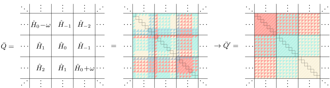
The quasienergy matrix retains its block structure, which can be visualized as follows:
| (8) | |||
Here, the matrices and are shown for the case of a three-level system for brevity, and . The central block describes the states of the central () FZ and their mutual couplings, which will be accounted for exactly. The off-diagonal blocks describe couplings between different Floquet zones; these couplings will be taken into account perturbatively. The connection between in Eq. (2) and in Eq. (8) is shown schematically in Fig. (1). The diagonal blocks no longer share common elements, with one possible exception in case there are states with reduced energies near both boundaries of the Floquet zones. For example, for the FZ choice , this will be the case if . The element of the th diagonal block will then coincide with the element of the st diagonal block. This issue will be discussed further in Section II.3. Abstracting from it, we proceed to derive the expressions for the effective Hamiltonian.
II.1 Extended degenerate perturbation theory
In the first step, we separate into the unperturbed part and the perturbation, the latter having a block-diagonal part and a block-off-diagonal one:
| (9) |
where
| (10) |
The dimensionless parameter has been introduced to track the order of the expansion. Inserting into Eq. (3) and assuming , one can collect the terms of the same order. In the first order, this yields
| (11) |
We require be block-off-diagonal, so that is block-off-diagonal as well. The remaining block-diagonal terms immediately yield the first-order term of the effective Hamiltonian according to
| (12) |
or, in the Hilbert space,
| (13) |
Next, we require , obtaining the equation for the block-off-diagonal terms: . This allows us to find and proceed to the equation for the second-order terms. Continuing in the similar fashion, one obtains
| (14) |
One recognizes that the resulting expressions are identical to the van Vleck high-frequency expansion [28], which is expected since possesses exactly the same structure as in the usual applications of this expansion. The Hilbert-space expressions, however, do different because the matrix elements of and the quantities have a different meaning in our case. The second-order term of the effective Hamiltonian results as
| (15) |
Expressions for the third-order terms of the effective Hamiltonian are provided in Appendix A.
The formula (14) could alternatively be obtained by a direct application of the conventional degenerate perturbation theory (DPT) widely used in the context of ordinary Hilbert space [31], provided one assumes that all of the states of a given block (, say) constitute the degenerate subspace. The condition in the summation over the intermediate states in Eq. (14) corresponds precisely to the skipping of states belonging to the degenerate subspace. We will refer to the Eqs. (13) and (15) as the results of the extended degenerate perturbation theory (EDPT) since the degenerate subspace is extended to include all levels in a Floquet zone.
II.2 Conventional degenerate perturbation theory
For comparison, let us consider the conventional DPT, whereby the degenerate subspace of consists only of the states that are exactly (or nearly) degenerate. We start by diving the Hilbert space into two subspaces, and , so that contains the states sharing the same value of reduced energy of interest, , while contains the remaining states. That is, for each state ,
| (16) |
Consequently, we partition each diagonal block of into two subblocks — one containing the states belonging to , and one containing the states of . The couplings between these subblocks are then considered to constitute the off-diagonal blocks of , and are therefore treated as a perturbation. This means that the definition of diagonal and off-diagonal blocks is changed from the one given in Eq. (10) to
| (17) |
Here, and so that the Kronecker delta is unity if both states and belong to the same subspace — either degenerate or not — and zero if they belong to different subspaces. With these definitions, and as before, one finds
| (18) |
in the first order and
| (19) |
in the second. In the last expression, is the subspace number which belongs to, i.e., . The terms of the effective Hamiltonian constructed using DPT are denoted here by , and they are composed of two uncoupled blocks. In fact, when using DPT, one is only interested in the block describing the degenerate subspace, and it can be diagonalized separately from the other block.
Notably, construction of is not equivalent to simply neglecting in the couplings between the blocks and . Considering two states and of the degenerate subspace, one has . This point will be discussed further in Section III.2.
The above formalism also allows one to construct schemes that are intermediate between DPT and EDPT. Instead of including in only the states whose reduced energies are equal to the reduced energy of interest , one can include all states in a certain interval (with ). The size of will then increase, resulting in larger numerical effort required to calculate the eigenvalues, but these should approximate the exact values more accurately. The choice corresponds to EDPT, whereby all states are assigned to . We will not, however, consider the accuracy of these intermediate schemes further in this work, instead focusing on the two limiting cases, DPT and EDPT.
II.3 Convergence condition
It follows that the necessary condition for the convergence of the expansion (3) is
| (20) |
which has to be satisfied for all states , and all integers , except those excluded in the summation in Eq. (15) (EDPT case) or Eq. (19) (DPT case). As long as the numerator does not vanish, this condition might be violated for , which is possible if the reduced energies of the two states and are on the opposite boundaries of the FZ. A simple resolution is to shift the FZ in a such way so that there are no levels near one or both boundaries. However, if the reduced energies fill the FZ densely, then the problem cannot be circumvented. The EDPT will be applicable in those cases only if the couplings between states on the boundary of the FZ can be disregarded. On the other hand, in case of DPT this issue does not arise for the states of the degenerate subspace if one centers the FZ around . Since and enumerate only the states of the degenerate subspace, the absolute values of denominators in Eq. (19) are no smaller than . However, the problem appears in the DPT case as well once the third-order term, provided in Appendix A, is included since it contains differences between the reduced energies of the nondegenerate subspace.
III Applications
To check the validity of the presented theories, we will compare the quasienergy spectra obtained by diagonalizing and with the numerically exact ones. The latter were obtained by diagonalizing the single-period evolution operator, calculated by propagating the Schrödinger equation [34]. The theory will be applied to a driven Bose–Hubbard system, defined in Section III.1.
III.1 Driven Bose–Hubbard model
The driven Bose–Hubbard model is defined by the Hamiltonian [35]
| (21) |
where , , and control the strengths of, respectively, the nearest-neighbor hopping, the on-site interaction, and the external driving (we study monochromatic driving of frequency ). The first sum runs over nearest-neighbor pairs, while the remaining ones run over all lattice sites. In the last sum, is the -coordinate of site , in units of the lattice constant. A gauge transformation with shows that the effect of the driving amounts to a renormalization of the hopping strength [26]:
| (22) |
The Fourier image of the resulting Hamiltonian is given by
| (23) |
where denotes the Bessel function of the first kind of order .
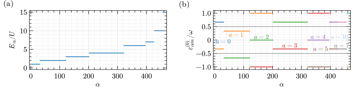
We will use the Fock basis to refer to the elements of , denoting the diagonal ones by . An example of the distribution of diagonal elements is displayed in Fig. 2(a). The presence of degenerate elements does not require extra care — these degeneracies will directly translate into degeneracies in the first-order term (14) of the effective Hamiltonian. The effective Hamiltonian, once obtained perturbatively, will be diagonalized exactly (numerically). On the other hand, the possibility of resonant transitions requires the application of degenerate perturbation theory in . Since the diagonal elements are given by integer multiples of , resonant transitions become possible when the condition , where , is satisfied. This translates into degeneracies in , as depicted in Fig. 2(b) showing the diagonal elements [see Eq. (6)] for . In the figure, black horizontal lines delimit the FZ chosen as , and the values of are displayed.
The analysis of accuracy of DPT and EDPT will be performed by choosing the driving strength and the frequency , and calculating the quasienergies as the parameter is varied. We will focus our attention on the quasienergy of the “driven Mott-insulator (MI) state”, a name we will use for the Floquet mode having the largest overlap with MI state (denoted as ). For , is the ground state of the undriven system, corresponding to . Therefore, we center the FZ around by choosing the interval .
We note that the interesting features of the quasienergy spectra — the anticrossings indicatory of resonant processes — will appear at certain values of the ratio . From the definition (5) with where is integer, it follows that the denominator in Eq. (20), , grows linearly in for fixed . Therefore, the accuracy of the perturbation theory in the vicinity of resonances is expected to increase with increasing , although this reasoning does not take into account the dependence on of the coupling strength [i.e. the numerator in Eq. (20)].
Finally, let us clarify that DPT can be applied not only exactly on resonance (when the degenerate energies of interest exactly coincide), but also in its vicinity. For example, we can calculate the quasienergies for in the vicinity of by including in the same states as those constituting when exactly equals . Similarly, the same reduction numbers [see Eq. (5)] as those obtained exactly on resonance are used even when does not exactly equal .
III.2 Study case 1: One-dimensional lattice
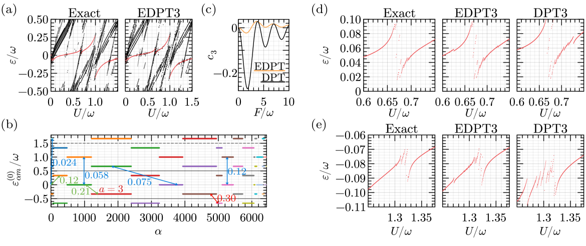
We begin the assessment of accuracy of the perturbation theories with the study of a BH system defined on a periodic lattice containing 8 bosons; we set and . The plots in Fig. 3(a) display the quasienergies of ten Floquet modes having the largest overlap with the MI state for . The quasienergies of the driven MI state are highlighted in red. The left plot displays the exact result, while the right one shows the results obtained using third-order EDPT. As explained above, the DPT approach is only applicable in the vicinity of resonances, and cannot be directly used to calculate the quasienergies for such a wide range of . The most pronounced anticrossing seen at corresponds to first-order creation of particle–hole excitations in the MI state, whereby a particle is annihilated at a certain site and created at its neighboring site [32]. At , transitions between all levels of the system become resonant, therefore, all diagonal elements of in the given diagonal block share the same value. Consequently, the actual distribution of quasienergies is almost entirely captured by the first-order effective Hamiltonian (13). Additionally, DPT becomes equivalent to EDPT since all levels of the system are included in the degenerate subspace. The second- and third-order terms of provide a slight improvement and yield results in agreement with the exact ones, as shown in Fig. 3(a). Notably, the EDPT results remain sufficiently accurate away from resonances as well. Exactly on the resonance , the largest value of the coupling ratio (20) is , which is one of the largest values that can be considered to satisfy the condition (20). Therefore, for smaller values of (and the same value of ), the EDPT is not expected to yield reliable results near the resonance .
To assess the accuracy of the methods on a finer scale, we inspect the quasienergy of the driven MI state in the vicinity of , as shown in Fig. 3(d). The obtained anticrossing is a result of the second-order process whereby two particles of an MI state hop to the site of their common neighbor, producing a triply occupied site and resulting in a state of energy . This process has been analyzed in Ref. [32] using the DPT approach. Plugging the expressions (23) into Eq. (19) one finds that for the resonance condition , the element vanishes for odd ( denotes any one of the states with a triply occupied site reachable starting from in two hops). Meanwhile, for , the strongest coupling is observed for . The quasienergy of the driven MI state is indeed calculated correctly using DPT, as shown in Fig. 3(d). However, as is tuned away from resonance, the EDPT yields more accurate results.
As noted in Section II.2, the EDPT and DPT approaches are not equivalent, therefore, the value of depends on which method is used to construct the effective Hamiltonian. These values are compared in Fig. 3(c) for and a range of coupling strengths . The curves are quite different in nature: for example, at the DPT curve crosses the zero, while the EDPT curve approaches a local maximum. Vanishing coupling indicates disappearance of the corresponding anticrossing in the quasienergy spectrum [32], which is indeed the case for , as confirmed by an exact calculation (not shown). Thus, even though EDPT yields quasienergies with higher accuracy than DPT, the matrix elements of constructed using EDPT do not have such a straightforward interpretation compared to the case when DPT is used. Another difference between EDPT and DPT concerns the higher-order terms of the effective Hamiltonian. In the DPT case, the third-order term gives an insignificant correction to the second-order theory at . The additional processes appearing in the third-order are the creation of a state featuring three doubly occupied sites (the corresponding matrix element is times smaller than ) and the process of creating a state with a triply occupied site in three hops (). In the EDPT case, on the other hand, inclusion of the third-order term gives a substantial improvement in terms of accuracy.
It is instructive to consider the values of the coupling ratios (20) for EDPT. Exactly on resonance , we find , which is quite large. However, this value comes from the coupling of a state corresponding to with a state corresponding to , therefore, this coupling does not directly influence the driven MI state, whose reduced energy is . The said coupling is indicated in red in Fig. 3(b) depicting the diagonal elements of at . On the other hand, all of the degenerate states sharing the value are coupled weakly to states outside the central FZ, as indicated by the blue numbers in Fig. 3(b) (see figure caption for details). This explains the fact that accurate results have been obtained using EDPT despite the condition (20) not being satisfied. We remind that the couplings between the states in the central FZ [see green arrows with numbers in Fig. 3(b)] are taken into account exactly in the EDPT framework. Meanwhile, the couplings of degenerate states with the nondegenerate ones are treated perturbatively in the DPT, which explains why the reported DPT results are less accurate even exactly on resonance.
Let us also discuss the origin of the discontinuity at in the EDPT results seen in Fig. 3(d). For definiteness, consider the group of levels characterized by and reduction number , appearing in red in Fig. 3(b), where is assumed. These are the levels arising from the unperturbed states of energy . As decreases, these levels shift downwards, reaching the lower FZ boundary when attains the value of . Decreasing still further makes this particular group of levels leave the FZ, and another one (appearing in green in the figure) enters from above. However, the reduction number for the levels of the latter group is . Since the reduction number directly influences the strength of coupling with other levels, the coupling with the states under consideration changes abruptly as crosses the value of . Although processes such as this one reduce the accuracy of the EDPT, their impact is not that noticeable if the states of actual interest are not strongly coupled to the states crossing the boundaries of FZ. This is certainly the case presently: Our main focus is on the driven MI state, which is not directly coupled to the states. Consequently, the artifactual discontinuity in Fig. 3(d) is an order of magnitude narrower than the width of the anticrossing that is of actual interest.
The last case for this parameter set is studied in Fig. 3(e) that displays the quasienergy of the driven MI state in the vicinity of . The anticrossing is again a manifestation of the second-order process producing a triply occupied site. Despite the width of the anticrossing making up only of the width of the FZ, it can be calculated accurately using perturbation theory. Again, EDPT is more accurate than DPT, although the former one yields a number of false anticrossings.
III.3 Study case 2: Two-dimensional lattice
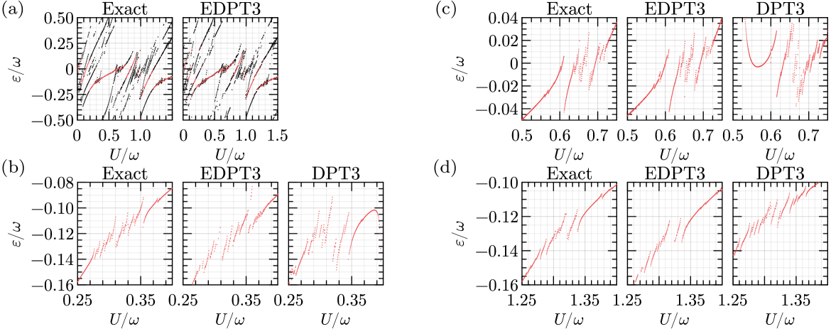
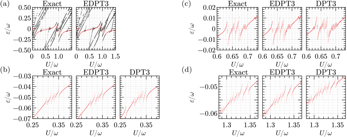
We now turn to a BH system described by the same parameter values (, ), but this time on a lattice periodic in the -direction (we direct the -axis along the longer dimension of the lattice). The quasienergy spectrum calculated for is shown in Fig. 4(a). We notice that the curve of the driven MI state undergoes many more anticrossings compared to the above case of a one-dimensional lattice, indicating richer system dynamics. The EDPT results are less accurate here, featuring erroneous and noticeable discontinuities. Nevertheless, the quasienergies can be considered calculated qualitatively correctly in the vicinity of the main anticrossing at .
According to Eq. (22), driving renormalizes the hopping strength only for hopping along the -axis. As a result, the DPT theory no longer predicts that vanishes for all when with odd. Indeed, Fig. 4(b) confirms that numerous anticrossings appear in the vicinity of . Their presence is predicted by both EDPT and DPT, albeit the exact results are matched only qualitatively. Meanwhile, in the cases and the EDPT ensures higher accuracy, providing a considerable improvement over DPT [see Figs. 4(c) and (d)].
Finally, we consider the results obtained for the case of a higher driving frequency: . As expected, the accuracy of the perturbation theory is higher in this case, which is confirmed by the plots in Fig. 5. Figure 5(a) shows that EDPT yields accurate results on a large scale, capturing all the essential features of the exact quasienergy spectrum. The close-up views of the spectrum in the vicinity of , and , shown in Figs. 5(b), (c), and (d), respectively, display that EDPT is capable of providing quantitatively correct results in this regime. The DPT is certainly applicable as well, although the accuracy is lower.
III.4 Computational cost of the methods
Concluding the discussion of accuracy of the considered methods, let us compare the associated computational costs. Calculation of quasienergies using both DPT and EDPT comes down to a Hermitian matrix diagonalization. In the EDPT case, one is required to diagonalize the matrix whose size is given by the total number of states of the unperturbed systems. In the studied eight-particle systems, there are such states. In the DPT case, the size is given by the number of states sharing the same value of reduced energy . For example, on a lattice and at , there are 2017 states sharing the value of [cf. Fig. 3(b)]. Both methods thus suffer from exponential growth of the required computation resources, which can only be alleviated by limiting the number of states taken into consideration.
The numerically exact calculation of the quasienergies via the single-period evolution operator requires performing a (unitary) matrix diagonalization, similarly to the the EDPT case. However, the construction of additionally requires propagating the Schrödinger equation for one period of the drive times (for each basis state as the initial condition). Although the specific time required to solve the differential equations depends on multiple factors (such as the solver, required tolerance, and hardware), in our experience [36] the exact calculation of the quasienergies for a single value of took 2.5–6 times longer than the EDPT calculation and, importantly, required times more memory (see Appendix B for details).
IV Conclusion
Let us now summarize the results. We have provided an extension of the conventional degenerate perturbation theory that improves the accuracy of the calculation of quasienergy spectra of periodically driven systems. Application of the theory to the driven Bose–Hubbard system has shown that third-order EDPT yields results matching the exact ones on a quantitative level. While the exact applicability criterion is difficult to formulate, the simple condition (20) together with the provided example calculations may serve as a basis for predicting the expected accuracy. Generally, the accuracy is expected to improve with increasing driving frequency.
Along the way, we have also studied the application of the conventional DPT. It has an advantage that the matrix elements of the resulting effective Hamiltonian admit a straightforward interpretation. Specifically, it enables one to make qualitative predictions about the possible appearance of the anticrossings in the quasienergy spectrum, and the matrix elements of may be used to estimate the relative probabilities of various resonant excitation processes [32, 33, 28]. On the other hand, since consists of two decoupled blocks (describing Hilbert spaces and , cf. Section II.2), which is clearly a bold approximation, it might not capture important properties of the system, such as the existence of a Floquet dynamical symmetry [37, 38, 39]. In this respect, the effective Hamiltonian provided by EDPT is expected to be more useful: existence of an operator such that with a real number would imply the existence of a dynamical symmetry in the effective system [37, 40], to the th order of the perturbation theory. This might help in exploring the platforms for constructing discrete time crystals.
The performed analysis has shown that the accuracy of the quasienergies obtained using DPT is considerably lower than that of EDPT. Moreover, while DPT is applicable only in the vicinity of resonances, EDPT remains equally useful if the driving is not resonant. The advantages of EDPT, however, come at the expense of increased numerical effort since the resulting effective Hamiltonian is of the same size as the unperturbed one. For large systems, its diagonalization becomes prohibitively costly, and one might need to reduce the number of considered states by excluding highly-excited ones, for example. Another option is to adopt a scheme intermediate between DPT and EDPT so that only some of the couplings between the states in the FZ are treated exactly, and others are taken into account perturbatively. The required formalism has been presently provided.
Appendix A: Third-order expressions for the effective Hamiltonian
Here, we provide the third-order expressions for the effective Hamiltonians. In the DPT framework, one obtains
| (A1) |
Here, integers , , , and indicate which subspaces the states belong to: , , , . In the EDPT framework, all states are assigned to the same subspace, therefore, in that case one should put in the above equation.
Appendix B: Benchmarks of the methods
In this Appendix we provide benchmarks of the methods and additional technical details.
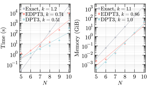
The scaling of the computational time and required memory with the system size is shown in Fig. 6. The performed calculations correspond to those presented in Fig. 3 at a single point of , for lattice sizes through 10 (with unit filling). The data is depicted on a semi-logarithmic scale, together with an exponential fit ; the coefficients are provided in the legends. It is apparent that the EDPT provides a noticeable advantage in terms of calculation times compared to the exact approach and requires more than an order of magnitude less memory. The memory requirements for DPT are similar to those of EDPT because we were constructing the effective Hamiltonian for both the degenerate and nondegenerate subspaces, although we were diagonalizing only the block corresponding to the degenerate space.
In practice, one often needs to repeat the calculation of quasienergies for a range of one or more system parameters, as was done in our analysis in the main text.
The loop scanning over the parameters can be easily parallelized on a multicore machine or a cluster, but the memory requirements might put a limit on the number of processes that can be run in parallel. For example, the exact calculation shown in Fig. 4(a), where values of were scanned, was performed using only 21 of 64 cores of an AMD 2990WX CPU because that already used almost all available RAM space (121 GB out of 128 GB). The execution time was 6 hours. Meanwhile, EDPT3 allowed us to utilize all 64 cores while requiring 22 GB RAM in total; the calculation finished in 50 minutes.
References
- Bukov et al. [2015a] M. Bukov, S. Gopalakrishnan, M. Knap, and E. Demler, Prethermal Floquet steady states and instabilities in the periodically driven, weakly interacting Bose-Hubbard model, Phys. Rev. Lett. 115, 205301 (2015a), arXiv:1507.01946 .
- Abanin et al. [2017] D. A. Abanin, W. De Roeck, W. W. Ho, and F. Huveneers, Effective Hamiltonians, prethermalization, and slow energy absorption in periodically driven many-body systems, Phys. Rev. B 95, 014112 (2017), arXiv:1510.03405 .
- Singh et al. [2019] K. Singh, C. J. Fujiwara, Z. A. Geiger, E. Q. Simmons, M. Lipatov, A. Cao, P. Dotti, S. V. Rajagopal, R. Senaratne, T. Shimasaki, M. Heyl, A. Eckardt, and D. M. Weld, Quantifying and controlling prethermal nonergodicity in interacting Floquet matter, Phys. Rev. X 9, 041021 (2019), arXiv:1809.05554 .
- Rubio-Abadal et al. [2020] A. Rubio-Abadal, M. Ippoliti, S. Hollerith, D. Wei, J. Rui, S. L. Sondhi, V. Khemani, C. Gross, and I. Bloch, Floquet prethermalization in a Bose-Hubbard system, Phys. Rev. X 10, 021044 (2020), arXiv:2001.08226 .
- Fleckenstein and Bukov [2021] C. Fleckenstein and M. Bukov, Prethermalization and thermalization in periodically driven many-body systems away from the high-frequency limit, Phys. Rev. B 103, L140302 (2021), arXiv:2012.10405 .
- Ho et al. [2023] W. W. Ho, T. Mori, D. A. Abanin, and E. G. Dalla Torre, Quantum and classical Floquet prethermalization, Ann. Phys. 454, 169297 (2023), arXiv:2212.00041 .
- Dunlap and Kenkre [1986] D. H. Dunlap and V. M. Kenkre, Dynamic localization of a charged particle moving under the influence of an electric field, Phys. Rev. B 34, 3625 (1986).
- Eckardt et al. [2009] A. Eckardt, M. Holthaus, H. Lignier, A. Zenesini, D. Ciampini, O. Morsch, and E. Arimondo, Exploring dynamic localization with a Bose-Einstein condensate, Phys. Rev. A 79, 013611 (2009), arXiv:0812.1997 .
- Bordia et al. [2017] P. Bordia, H. Lüschen, U. Schneider, M. Knap, and I. Bloch, Periodically driving a many-body localized quantum system, Nat. Phys. 13, 460 (2017), arXiv:1607.07868 .
- Abanin et al. [2019] D. A. Abanin, E. Altman, I. Bloch, and M. Serbyn, Colloquium: Many-body localization, thermalization, and entanglement, Rev. Mod. Phys. 91, 021001 (2019), arXiv:1804.11065 .
- Kitagawa et al. [2010] T. Kitagawa, E. Berg, M. Rudner, and E. Demler, Topological characterization of periodically driven quantum systems, Phys. Rev. B 82, 235114 (2010), arXiv:1010.6126 .
- Grushin et al. [2014] A. G. Grushin, Á. Gómez-León, and T. Neupert, Floquet fractional Chern insulators, Phys. Rev. Lett. 112, 156801 (2014), arXiv:1309.3571 .
- Jotzu et al. [2014] G. Jotzu, M. Messer, R. Desbuquois, M. Lebrat, T. Uehlinger, D. Greif, and T. Esslinger, Experimental realization of the topological Haldane model with ultracold fermions, Nature 515, 237 (2014), arXiv:1406.7874 .
- Mikami et al. [2016] T. Mikami, S. Kitamura, K. Yasuda, N. Tsuji, T. Oka, and H. Aoki, Brillouin-Wigner theory for high-frequency expansion in periodically driven systems: Application to Floquet topological insulators, Phys. Rev. B 93, 144307 (2016), arXiv:1511.00755 .
- Price et al. [2017] H. M. Price, T. Ozawa, and N. Goldman, Synthetic dimensions for cold atoms from shaking a harmonic trap, Phys. Rev. A 95, 023607 (2017), arXiv:1605.09310 .
- Sacha [2015] K. Sacha, Modeling spontaneous breaking of time-translation symmetry, Phys. Rev. A 91, 033617 (2015).
- Else et al. [2016] D. V. Else, B. Bauer, and C. Nayak, Floquet time crystals, Phys. Rev. Lett. 117, 090402 (2016), arXiv:1603.08001 .
- Yao et al. [2017] N. Y. Yao, A. C. Potter, I.-D. Potirniche, and A. Vishwanath, Discrete time crystals: Rigidity, criticality, and realizations, Phys. Rev. Lett. 118, 030401 (2017), arXiv:1608.02589 .
- Zhang et al. [2017] J. Zhang, P. W. Hess, A. Kyprianidis, P. Becker, A. Lee, J. Smith, G. Pagano, I.-D. Potirniche, A. C. Potter, A. Vishwanath, N. Y. Yao, and C. Monroe, Observation of a discrete time crystal, Nature 543, 217 (2017), arXiv:1609.08684 .
- Choi et al. [2017] S. Choi, J. Choi, R. Landig, G. Kucsko, H. Zhou, J. Isoya, F. Jelezko, S. Onoda, H. Sumiya, V. Khemani, C. von Keyserlingk, N. Y. Yao, E. Demler, and M. D. Lukin, Observation of discrete time-crystalline order in a disordered dipolar many-body system, Nature 543, 221 (2017), arXiv:1610.08057 .
- Else et al. [2020] D. V. Else, C. Monroe, C. Nayak, and N. Y. Yao, Discrete Time Crystals, Annu. Rev. Condens. Matter Phys. 11, 467 (2020), arXiv:1905.13232 .
- Shirley [1965] J. H. Shirley, Solution of the Schrödinger equation with a Hamiltonian periodic in time, Phys. Rev. 138, B979 (1965).
- Sambe [1973] H. Sambe, Steady states and quasienergies of a quantum-mechanical system in an oscillating field, Phys. Rev. A 7, 2203 (1973).
- Goldman and Dalibard [2014] N. Goldman and J. Dalibard, Periodically driven quantum systems: Effective Hamiltonians and engineered gauge fields, Phys. Rev. X 4, 031027 (2014), arXiv:1404.4373 .
- Bukov et al. [2015b] M. Bukov, L. D’Alessio, and A. Polkovnikov, Universal high-frequency behavior of periodically driven systems: From dynamical stabilization to Floquet engineering, Adv. Phys. 64, 139 (2015b), arXiv:1407.4803 .
- Eckardt [2017] A. Eckardt, Colloquium: Atomic quantum gases in periodically driven optical lattices, Rev. Mod. Phys. 89, 011004 (2017), arXiv:1606.08041 .
- Rahav et al. [2003] S. Rahav, I. Gilary, and S. Fishman, Effective Hamiltonians for periodically driven systems, Phys. Rev. A 68, 013820 (2003), arXiv:nlin/0301033 .
- Eckardt and Anisimovas [2015] A. Eckardt and E. Anisimovas, High-frequency approximation for periodically driven quantum systems from a Floquet-space perspective, New J. Phys. 17, 093039 (2015), arXiv:1502.06477 .
- Itin and Katsnelson [2015] A. P. Itin and M. I. Katsnelson, Effective Hamiltonians for rapidly driven many-body lattice systems: Induced exchange interactions and density-dependent hoppings, Phys. Rev. Lett. 115, 075301 (2015), arXiv:1401.0402 .
- Rodriguez-Vega et al. [2018] M. Rodriguez-Vega, M. Lentz, and B. Seradjeh, Floquet perturbation theory: Formalism and application to low-frequency limit, New J. Phys. 20, 093022 (2018), arXiv:1805.01190 .
- Landau and Lifshitz [1981] L. D. Landau and E. M. Lifshitz, Quantum Mechanics: Non-relativistic Theory, Course of Theoretical Physics, Vol. 3 (Butterworth-Heinemann, 1981).
- Eckardt and Holthaus [2008] A. Eckardt and M. Holthaus, Avoided-level-crossing spectroscopy with dressed matter waves, Phys. Rev. Lett. 101, 245302 (2008), arXiv:0809.1032 .
- Weinberg et al. [2015] M. Weinberg, C. Ölschläger, C. Sträter, S. Prelle, A. Eckardt, K. Sengstock, and J. Simonet, Multiphoton interband excitations of quantum gases in driven optical lattices, Phys. Rev. A 92, 043621 (2015), arXiv:1505.02657 .
- Holthaus [2015] M. Holthaus, Floquet engineering with quasienergy bands of periodically driven optical lattices, J. Phys. B: At., Mol. Opt. Phys. 49, 013001 (2015), arXiv:1510.09042 .
- Eckardt et al. [2005] A. Eckardt, C. Weiss, and M. Holthaus, Superfluid-insulator transition in a periodically driven optical lattice, Phys. Rev. Lett. 95, 260404 (2005), arXiv:cond-mat/0601020 .
- [36] See https://github.com/yakovbraver/FloquetSystems.jl for the package source code.
- Chinzei and Ikeda [2020] K. Chinzei and T. N. Ikeda, Time crystals protected by Floquet dynamical symmetry in Hubbard models, Phys. Rev. Lett. 125, 060601 (2020), arXiv:2003.13315 .
- Sarkar and Dubi [2022a] S. Sarkar and Y. Dubi, Signatures of discrete time-crystallinity in transport through an open Fermionic chain, Commun Phys 5, 155 (2022a), arXiv:2107.04214 .
- Sarkar and Dubi [2022b] S. Sarkar and Y. Dubi, Emergence and dynamical stability of a charge time-crystal in a current-carrying quantum dot simulator, Nano Lett. 22, 4445 (2022b), arXiv:2205.06441 .
- Buča et al. [2019] B. Buča, J. Tindall, and D. Jaksch, Non-stationary coherent quantum many-body dynamics through dissipation, Nat Commun 10, 1730 (2019), arXiv:1804.06744 .
- Rackauckas and Nie [2017] C. Rackauckas and Q. Nie, DifferentialEquations.jl – a performant and feature-rich ecosystem for solving differential equations in Julia, J. Open Res. Software 5, 15 (2017).
- Rackauckas and Nie [2019] C. Rackauckas and Q. Nie, Confederated modular differential equation APIs for accelerated algorithm development and benchmarking, Adv. Eng. Software 132, 1 (2019), arXiv:1807.06430 .
- Tsitouras [2011] Ch. Tsitouras, Runge–Kutta pairs of order 5(4) satisfying only the first column simplifying assumption, Comput. Math. Appl. 62, 770 (2011).
- Bezanson et al. [2017] J. Bezanson, A. Edelman, S. Karpinski, and V. B. Shah, Julia: A fresh approach to numerical computing, SIAM Rev. 59, 65 (2017), arXiv:1411.1607 .