Extended Fiducial Inference for Individual Treatment Effects via Deep Neural Networks
Abstract
Individual treatment effect estimation has gained significant attention in recent data science literature. This work introduces the Double Neural Network (Double-NN) method to address this problem within the framework of extended fiducial inference (EFI). In the proposed method, deep neural networks are used to model the treatment and control effect functions, while an additional neural network is employed to estimate their parameters. The universal approximation capability of deep neural networks ensures the broad applicability of this method. Numerical results highlight the superior performance of the proposed Double-NN method compared to the conformal quantile regression (CQR) method in individual treatment effect estimation. From the perspective of statistical inference, this work advances the theory and methodology for statistical inference of large models. Specifically, it is theoretically proven that the proposed method permits the model size to increase with the sample size at a rate of for some , while still maintaining proper quantification of uncertainty in the model parameters. This result marks a significant improvement compared to the range required by the classical central limit theorem. Furthermore, this work provides a rigorous framework for quantifying the uncertainty of deep neural networks under the neural scaling law, representing a substantial contribution to the statistical understanding of large-scale neural network models.
Keywords: Causal Inference, Deep Learning, Fiducial Inference, Stochastic Gradient MCMC, Uncertainty Quantification
1 Introduction
Causal inference is a fundamental problem in many disciplines such as medicine, econometrics, and social science. Formally, let denote a set of observations drawn from the following data-generating equations:
| (1) |
where represents a vector of covariates of subject , represents the treatment assignment to subject ; represents the expected outcome of subject if assigned to the control group (with , and is the expected treatment effect of subject if assigned to the treatment group (with ); is the standard deviation, and represent a standardized random error that is not necessarily Gaussian. Under the potential outcome framework (Rubin, 1974), each individual receives only one assignment of the treatment with or 1, but not both. The goal of causal inference is to make inference for the average treatment effect (ATE) or individual treatment effect (ITE).
The ATE is defined as
| (2) |
where denotes the sample space of , and denotes the cumulative distribution function of . To estimate ATE, a variety of methods, including outcome regression, augmented/inverse probability weighting (AIPW/IPW) and matching, have been developed. See Imbens (2004) and Rosenbaum (2002) for overviews.
The ITE is often defined as the conditional average treatment effect (CATE):
| (3) |
see e.g., Shalit et al. (2017) and Lu et al. (2018). Recently, Lei and Candès (2021) proposed to make predictive inference of the ITE by quantifying the uncertainty of
| (4) |
where denotes the potential outcome of subject with treatment assignment . Henceforth, we will call the predictive ITE.
It is known that ATE and ITE are identifiable if the conditions ‘strong ignorability’ and ‘overlapping’ are satisfied. The former means that, after accounting for observed covariates, the treatment assignment is independent of potential outcomes; and the latter ensures that every subject in the study has a positive probability of receiving either assignment, allowing for meaningful comparisons between treatment and control groups. Mathematically, the two conditions can be expressed as:
where represents the treatment assignment variable, and denotes conditional independence. Together, they ensure that the causal effect can be correctly estimated without bias. See e.g. Guan and Yang (2019) for more discussions on this issue.
However, even under these assumptions, accurate inference for ATE and ITE can still be challenging. Specifically, the inference task can be complicated by unknown nonlinear forms of and . To address these issues, some authors have proposed to approximate them using a machine learning model, such as random forest (RF) (Breiman, 2001), Bayesian additive regression trees (BART) (Chipman et al., 2010), and neural networks. Refer to e.g., Foster et al. (2011), Hill (2011), Shalit et al. (2017), Wager and Athey (2018), and Hahn et al. (2020) for the details. Unfortunately, these methods often yield point estimates for the ATE and ITE, while failing to correctly quantifying their uncertainty due to the complexity of the machine learning models. Quite recently, Lei and Candès (2021) proposed to quantify the uncertainty of the predictive ITE using the conformal inference method (Vovk et al., 2005; Shafer and Vovk, 2008). This method provides coverage-guaranteed confidence intervals for the predictive ITE, but the intervals may become overly wide when the machine learning model is not consistently estimated. In short, while machine learning models, particularly neural networks, can effectively model complex, nonlinear functions such as and for causal inference, performing accurate uncertainty quantification with these models remains a significant challenge. This is because these models typically have a complex functional form and involve a large number of parameters.
In this paper, we propose to conduct causal inference using an extended fiducial inference (EFI) method (Liang et al., 2024), with the goal of addressing the uncertainty quantification issue associated with treatment effect estimation. EFI provides an innovative framework for inferring model uncertainty based solely on observed data, aligning with the goal of fiducial inference (Fisher, 1935; Hannig, 2009). Specifically, it aims to solve the data-generating equations by explicitly imputing the unobserved random errors and approximating the model parameters from the observations and imputed random errors using a neural network; it then infers the uncertainty of the model parameters based on the learned neural network function and the imputed random errors (see Section 2 for a brief review). To make the EFI method feasible for causal effect estimation with accurate uncertainty quantification, we extend the method in two key aspects:
-
(i)
We approximate each of the unknown functions, and , by a deep neural network (DNN) model. The DNN possesses universal approximation capability (Hornik et al., 1989; Hornik, 1991; Kidger and Lyons, 2020), meaning it can approximate any continuous function to an arbitrary degree of accuracy, provided it is sufficiently wide and deep. This property makes the proposed method applicable to a wide range of data-generating processes.
-
(ii)
We theoretically prove that the dimensions (i.e., the number of parameters) of the DNN models used to approximate and are allowed to increase with the sample size at a rate of for some , while the uncertainty of the DNN models can still be correctly quantified. That is, we are able to correctly quantify the uncertainty of the causal effect although it has to be approximated using large models.
In this paper, we regard a model as ‘large’ if its dimension increases with at a rate of . We note that part (ii) represents a significant theoretical innovation in statistical inference for large models. In the literature on this area, most efforts have focused on linear models, featuring techniques such as desparsified Lasso (Javanmard and Montanari, 2014; van de Geer et al., 2014; Zhang and Zhang, 2014), post-selection inference (Lee et al., 2016), and Markov neighborhood regression (Liang et al., 2022a). For nonlinear models, the research landscape appears to be more scattered. Portnoy (1986, 1988) showed that for independently and identically distributed (i.i.d) random vectors with the dimension increasing with the sample size , the central limit theorem (CLT) holds if for some . It is worth noting that Bayesian methods, despite being sampling-based, do not permit the dimension of the true model to increase with at a higher rate. For example, even in the case of generalized linear models, to ensure the posterior consistency, the dimension of the true model is only allowed to increase with at a rate (see Theorem 2 and Remark 2 of Jiang (2007)). Under its current theoretical framework developed by Liang et al. (2024), EFI can only be applied to make inference for the models whose dimension is fixed or increases with at a very low rate. This paper extends the theoretical framework of EFI further, establishing its applicability for statistical inference of large models.
It is worth noting that a DNN model with size , where is close to (but less than) 1, has been shown to be sufficiently large for approximating many data generation processes. This is supported by the theory established in Sun et al. (2022) and Farrell et al. (2021). In Sun et al. (2022), it is shown that, as , a sparse DNN model of this size can provide accurate approximations for multiple classes of functions, such as bounded -Hölder smooth functions (Schmidt-Hieber, 2020), piecewise smooth functions with fixed input dimensions (Petersen and Voigtlaender, 2018), and functions representable by an affine system (Bolcskei et al., 2019). Similar results have also been obtained in Farrell et al. (2021), where it is shown that a multi-layer perceptron (MLP) with this model size and the ReLU activation function can provide an accurate approximation to the functions that lie in a Sobolev ball with certain smoothness. The approximation capability of DNNs of this size has also been empirically validated by Hestness et al. (2017), where a neural scaling law of with was identified through extensive studies across various model architectures in machine translation, language modeling, image processing, and speech recognition.
To highlight the strength of EFI in uncertainty quantification and to facilitate comparison with the conformal inference method, this study focuses on inference for predictive ITEs, although the proposed method can also be extended to ATE and CATE. Our numerical results demonstrate the superiority of the proposed method over the conformal inference method.
The remaining part of this paper is organized as follows. Section 2 provides a brief review of the EFI method. Section 3 extends EFI to statistical inference for large statistical models. Section 4 provides an illustrative example for EFI. Section 5 applies the proposed method to statistical inference for predictive ITEs, with both simulated and real data examples. Section 6 concludes the paper with a brief discussion.
2 A Brief Review of the EFI Method
While fiducial inference was widely considered as a big blunder by R.A. Fisher, the goal he initially set —inferring the uncertainty of model parameters on the basis of observations — has been continually pursued by many statisticians, see e.g. Zabell (1992), Hannig (2009), Hannig et al. (2016), Murph et al. (2022), and Martin (2023). To this end, Liang et al. (2024) developed the EFI method based on the fundamental concept of structural inference (Fraser, 1966, 1968). Consider a regression model:
| (5) |
where and represent the response and explanatory variables, respectively; represents the vector of parameters; and represents a scaled random error following a known distribution . For the model (1), the treatment assignment should be included as a part of .
Suppose that a random sample of size has been collected from the model, denoted by . In the point of view of structural inference (Fraser, 1966, 1968), they can be expressed in the data generating equations as follow:
| (6) |
This system of equations consists of unknowns, namely, , while there are only equations. Therefore, the values of cannot be uniquely determined by the data-generating equations, and this lack of uniqueness of unknowns introduces uncertainty in .
Let denote the unobservable random errors, which are also called latent variables in EFI. Let denote an inverse function/mapping for the parameter , i.e.,
| (7) |
It is worth noting that the inverse function is generally non-unique. For example, it can be constructed by solving any equations in (6) for . As noted by Liang et al. (2024), this non-uniqueness of inverse function mirrors the flexibility of frequentist methods, where different estimators of can be designed for different purposes.
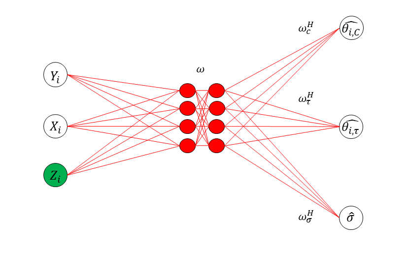
As a general method, Liang et al. (2024) proposed to approximate the inverse function using a sparse DNN, see Figure 1 for illustration. They also introduced an adaptive stochastic gradient Langevin dynamics (SGLD) algorithm, which facilitates the simultaneous training of the sparse DNN and simulation of the latent variables . This is briefly described as follows.
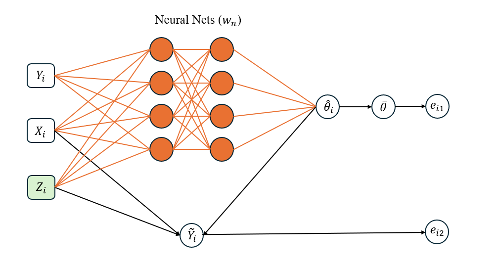
Let denote the DNN prediction function parameterized by the weights in the EFI network, and let
| (8) |
which serves as an estimator of . The EFI network has two output nodes defined, respectively, by
| (9) |
where , is as specified in (6), and is a function that measures the difference between and . For example, for a normal linear/nonlinear regression, it can be defined as
| (10) |
For logistic regression, it is defined as a squared ReLU function, see Liang et al. (2024) for the details. Furthermore, EFI defines an energy function as follows:
| (11) |
for some regularization coefficient , where first term measures the fitting error of the model as implied by equation (10), and the second term regularizes the variation of , ensuring that the neural network forms a proper estimator of the inverse function. Given this energy function, we define the likelihood function as
| (12) |
for some constant close to 0. As discussed in Liang et al. (2024), the choice of does not have much affect on the performance of EFI as long as is sufficiently small.
Subsequently, the posterior of is given by
| (13) |
where denotes the prior of ; and the predictive distribution of is given by
| (14) |
In EFI, is estimated through maximizing the posterior given the observations . By the Bayesian version of Fisher’s identity (Song et al., 2020), the gradient equation can be re-expressed as
| (15) |
which can be solved using an adaptive stochastic gradient MCMC algorithm (Liang et al., 2022b; Deng et al., 2019). The algorithm works by iterating between two steps:
-
(a)
Latent variable sampling: draw according to a Markov transition kernel that leaves to be invariant;
-
(b)
Parameter updating: update toward the maximum of using stochastic approximation (Robbins and Monro, 1951), based on the sample .
See Algorithm 1 for the pseudo-code. This algorithm is termed “adaptive” because the transition kernel in the latent variable sampling step changes with the working parameter estimate of . The parameter updating step can be implemented using mini-batch SGD, and the latent variable sampling step can be executed in parallel for each observation . Hence, the algorithm is scalable with respect to large datasets.
| (16) |
Under mild conditions for adaptive stochastic gradient MCMC algorithms (Deng et al., 2019; Liang et al., 2022b), it was shown in Liang et al. (2024) that
| (17) |
where denotes a solution to equation (15) and denotes convergence in probability, and that
| (18) |
in 2-Wasserstein distance, where denotes weak convergence.
To study the limit of (18) as decays to 0, i.e.,
where is referred to as the extended fiducial density (EFD) of learned in EFI, it is necessary for to be a consistent estimator of , the parameters of the underlying true EFI network. To ensure this consistency, Liang et al. (2024) impose some conditions on the structure of the DNN and the prior distribution . Specifically, they assume that takes values in a compact space ; is a truncated mixture Gaussian distribution on ; and the DNN structure satisfies certain constraints given in Sun et al. (2022), e.g., the width of the output layer (i.e., the dimension of ) is fixed or grows very slowly with . They then justify the consistency of based on the sparse deep learning theory developed in Sun et al. (2022). The consistency of further implies that
serves as a consistent estimator for the inverse function/mapping .
By Theorem 3.2 in Liang et al. (2024), for the target model (1), which is a noise-additive model, the EFD of is invariant to the choice of the inverse function, provided that is specified as in (10) in defining the energy function. Further, by Lemma 4.2 in Liang et al. (2024), is given by
| (19) |
where represents the cumulative distribution function (CDF) corresponding to ; represents the zero-energy set, which forms a manifold in the space ; and is the sum of intrinsic measures on the -dimensional manifold in . That is, under the consistency of , is reduced to a truncated density function of on the manifold , while itself is also invariant to the choice of the inverse function as shown in Lemma 3.1 of Liang et al. (2024). In other words, for the model (1), the EFD of is asymptotically invariant to the inverse function we learned given its consistency.
Let denote the parameter space of the target model, which represents the set of all possible values of that takes when runs over . Then, for any function of interest, its EFD associated with is given by
| (20) |
where . The EFD provides an uncertainty measure for . Practically, the EFD of can be constructed based on the samples , where denotes the fiducial -samples collected at step (iv) of Algorithm 1.
Finally, we note that, as discussed in Liang et al. (2024), the invariance property of is not crucial to the validity of EFI, although it does enhance the robustness of the inference. Additionally, for a neural network model, its parameters are only unique up to certain loss-invariant transformations, such as reordering hidden neurons within the same hidden layer or simultaneously altering the sign or scale of certain connection weights, see Sun et al. (2022) for discussions. Therefore, in EFI, the consistency of refers to its consistency with respect to one of the equivalent solutions to (15), while mathematically can still be treated as unique. Refer to Section 1.1 (of the supplement) for more discussions on this issue.
3 EFI for Large Models
In this section, we first establish the consistence of the inverse function/mapping learned in EFI for large models, and then discuss its application for uncertainty quantification of deep neural networks.
3.1 Consistency of Inverse Mapping Learned in EFI for Large Models
It is important to note that the sparse deep learning theory of Sun et al. (2022) is developed under the general constraint for some , which restricts the dimension of the output layer of the DNN model to be fixed or grows very slowly with the sample size . Therefore, under its current theoretical framework, EFI can only be applied to the models for which the dimension is fixed or increases very slowly with .
To extend EFI to large models, where the dimension of can grow with at a rate of , particularly for , we provide a new proof for the consistency of based on the theory of stochastic deep learning (Liang et al., 2022b). Specifically, we establish the following theorem, where the output layer width of the DNN in the EFI network is set to match the dimension of . The proof is lengthy and provided in the supplement.
Theorem 3.1
As implied by (21), we have holds for each layer . We call such a neural network a narrow DNN. For narrow DNNs, by the existing theory, see e.g., Kidger and Lyons (2020), Park et al. (2020), and Kim et al. (2023), the universal approximation can be achieved with a minimum hidden layer width of , where and represent the widths of the input and output layers, respectively. Hence, (21) implies that EFI can be applied to statistical inference for a large model of dimension
under the narrow DNN setting with the depth for some . Here, Without loss of generality, we assume . For such a DNN, the total dimension of :
can be much greater than , where ‘1’ represents the bias parameter of each neuron at the hidden and output layers. Specifically, we can have with appropriate choices of and . However, leveraging the asymptotic equivalence between the DNN and an auxiliary stochastic neural network (StoNet) (Liang et al., 2022b), we can still prove that the resulting estimator of is consistent, see the supplement for the detail.
Regarding this extension of the EFI method for statistical inference of large models, we have an additional remark:
Remark 1
In this paper, we impose a mixture Gaussian prior on to ensure the consistency of and, consequently, the consistency of the inverse mapping . However, this Bayesian treatment of is not strictly necessary, although it introduces sparsity that improves the efficiency of EFI. For the narrow DNN, the consistency of the estimator can also be established under the frequentist framework by leveraging the asymptotic equivalence between the DNN and the auxiliary StoNet, using the same technique introduced in the supplement (see Section 1.2). In this narrow and deep setting, each of the regressions formed by the StoNet is low-dimensional (with ), making the Bayesian treatment of unnecessary while still achieving a consistent estimator of .
3.2 Double-NN Method
Suppose a DNN is used for modeling the data, i.e., approximating the function in (5). By Sun et al. (2022) and Farrell et al. (2021), a DNN of size for some has been large enough for approximating many classes of functions. Therefore, EFI can be used for making inference for such a DNN model. In this case, EFI involves two neural networks, one is for modeling the data, which is called the ‘data modeling network’ and parameterized by ; and the other one is for approximating the inverse function, which is called the ‘inverse mapping network’ and parameterized by . Therefore, the proposed method is coined as ‘double-NN’. Note that during the EFI training process, only the parameters of the inverse mapping network are updated in equation (16) of Algorithm 1. The parameters of the data modeling network are subsequently updated in response to the adjustment of , based on the formula given in (8).
In our theoretical study for the double-NN method, we actually assume that the true data-generating model is a neural network, thereby omitting the approximation error of the data modeling network, based on its universal approximation capability. In practice, we have observed that the double-NN method is robust to this approximation error. Specifically, even when the true model is not a neural network, EFI can still recover the true random errors with high accuracy and achieve the zero-energy solution as and . A further theoretical exploration of this phenomenon would be of interest.
As mentioned previously, for a neural network model, its parameters are only unique up to certain loss-invariant transformations. As the training sample size becomes large, we expect that the optimizers are all equivalent. Thus, in this paper, the consistency of refers to its consistency with respect to one of the equivalent global optimizers, while mathematically can still be treated as unique. A similar issue occurs to the parameters of the inverse mapping network, as discussed in Section 1.1 of the supplement.
4 An Illustrative Example for EFI
To illustrate how EFI works for statistical inference problems, we consider a linear regression example:
| (22) |
where is a binary variable indicating the treatment assignment, is the treatment effect, are confounders/covariates, is the standardized random noise, and and are unknown parameters. For this example, represents the ATE as well as the CATE, due to its independence of the covariates . In the simulation study, we set , , , and ; generate ; and generate the treatment variable via a logistic regression:
| (23) |
where and . We consider three different cases with the sample size , 500 and 1000, respectively. For each case, we generate 100 datasets.
Statistical inference for the parameters in the model (22) can be made with EFI under its standard framework. Let be the parameter vector. EFI approximates the inverse function by a DNN, for which serves as input variables and as output variables. The results are summarized in Table 1.
For comparison, a variety of methods, including Unadj (Imbens and Rubin, 2015), inverse probability weighting (IPW) (Rosenbaum, 1987), double-robust (DR) (Robins et al., 1994; Bang and Robins, 2005), and BART (Hill, 2011), have been applied to this example. These methods fall into distinct categories. The Unadj is straightforward, estimating the ATE by calculating the difference between the treatment and control groups, i.e., , where the effect of confounders is not adjusted. Both IPW and DR are widely used ATE estimation methods, which adjust the effect of confounders based on propensity scores. They both are implemented using the R package drgee (Zetterqvist and Sjölander, 2015). The BART employs Bayesian additive regression trees to learn the outcome function, which naturally accommodates heterogeneous treatment effects as well as nonlinearity of the outcome function. It is implemented using the R package bartcause (Dorie and Hill, 2020).
| Method | coverage | length | coverage | length | coverage | length | ||
|---|---|---|---|---|---|---|---|---|
| Unadj | 0.95 | 1.161(0.066) | 0.93 | 0.822(0.032) | 0.97 | 0.424(0.017) | ||
| BART | 0.99 | 0.857(0.070) | 0.98 | 0.611(0.047) | 0.96 | 0.428(0.024) | ||
| IPW | 0.90 | 0.710(0.157) | 0.92 | 0.560(0.141) | 0.92 | 0.417(0.101) | ||
| DR | 0.96 | 0.652(0.058) | 0.93 | 0.465(0.033) | 0.94 | 0.331(0.017) | ||
| EFI | 0.95 | 0.647(0.033) | 0.95 | 0.438(0.021) | 0.95 | 0.338(0.012) | ||
The comparison indicates that EFI performs very well for this standard ATE estimation problem. Specifically, EFI generates confidence intervals of nearly the same length as DR, but with more accurate coverage rates. This is remarkable, as DR has often been considered as the golden standard for ATE estimation and is consistent if either the outcome or propensity score models is correctly specified, and locally efficient if both are correctly specified. Furthermore, EFI produces much shorter confidence intervals compared to Unadj, IPW, and BART, while maintaining more accurate coverage rates.
We attribute the superior performance of EFI on this example to its fidelity in parameter estimation, an attractive property of EFI as discussed in Liang et al. (2024). As implied by (14), EFI essentially estimates by maximizing the predictive likelihood function , which balances the likelihood of and the model fitting errors coded in . In contrast, the maximum likelihood estimation (MLE) method sets , where is expressed as a function of . In general, MLE is inclined to be influenced by the outliers and deviations of covariates especially when the sample size is not sufficiently large. It is important to note that the MLE serves as the core for all the IPW, DR and BART methods in estimating the outcome and propensity score models. For this reason, various adjustments for confounding and heterogeneous treatment effects have been developed in the literature.
Compared to the existing causal inference methods, EFI works as a solver for the data-generating equation (as ), providing a coherent way to address the confounding and heterogeneous treatment effects and resulting in faithful estimates for the model parameters and their uncertainty as well. This example illustrates the performance of EFI in ATE estimation when confounders are present, while the examples in the next section showcase the performance of EFI in dealing with heterogeneous treatment effects via DNN modeling. Extensive comparisons with BART and other nonparametric modeling methods are also presented.
In this example, we omit the estimation of the propensity score model. As discussed in Section 6, the proposed method can be extended by including an additional DNN to approximate the propensity score, enabling the use of inverse probability weighting for ATE estimation. However, the ATE estimation is not the focus of this work.
5 Causal Inference for Individual Treatment Effects
This section demonstrates how EFI can be used to perform statistical inference of the predictive ITE for the data-generating model (1). Let denote the vector of parameters for modeling the function , let denote the vector of parameters for modeling the function , and let denote the whole set of parameters for the model (1). We model the inverse function by a DNN. Also, we can model each of the functions and by a DNN if their functional forms are unknown. For convenience, we refer to the DNN for modeling as ‘-network’ and that for modeling as ‘-network’, and and represent their weights, respectively. As mentioned previously, we can restrict the sizes of the -network and -network to the order of for some .
Note that in solving the data generating equations (1), the proposed method involves two types of neural networks: one for modeling causal effects and the other for approximating the inverse function . While we still refer to the proposed method as ‘Double-NN’, it actually involves three DNNs.
5.1 ITE prediction intervals
Assume the training set consists of subjects, and the test set consists of subjects. The subjects in the test set can be grouped into three categories: (i) , , where the responses under the control are observed; (ii) , where the responses under the treatment are observed; and (iii) , where only covariates are observed. Here, we use , , and to denote the index sets of the subjects in the respective categories and, therefore, . For the ITE of each subject in the test set, we can construct the prediction interval with a desired confidence level of in the following procedure:
-
(i)
For subject : At each iteration of Algorithm 1, calculate the prediction , where . Let and denote, respectively, the - and -quantiles of collected over iterations. Since is observed, forms a -prediction interval for the ITE .
-
(ii)
For subject : At each iteration of Algorithm 1, calculate the prediction , where . Let and denote, respectively, the - and -quantiles of collected over iterations. Since is observed, forms a -prediction interval for the ITE .
-
(iii)
For subject : At each iteration of Algorithm 1, calculate the prediction , where . Let and denote, respectively, the - and -quantiles of collected over iterations. Then forms a -prediction interval for the ITE .
5.2 Simulation Study
Example 1
Consider the data-generating equation
| (24) |
where with each element drawn independently from , , , , , , and . As in Lei and Candès (2021), we set , and generate the treatment variable according to the propensity score model:
| (25) |
where is the CDF of the beta distribution with parameters (2,4), ensuring and thereby sufficient overlap between the treatment and control groups. In terms of equation (1), we have and . We generated 20 datasets from the model (24) independently, each consisting of training samples and test samples.
Case Case Case Method Coverage Length Coverage Length Method Coverage Length Double-NN 0.9549 4.2004 0.9581 4.1812 Double-NN 0.9583 5.6056 (0.0095) (0.1567) (0.0098) (0.1541) (0.0103) (0.2207) CQR-BART 0.9472 4.2702 0.9533 4.4024 CQR(inexact) 0.9530 6.3244 (0.0342) (0.5225) (0.0341) (0.8972) (0.0198) (0.5426) CQR-Boosting 0.9556 5.5199 0.9548 4.4493 CQR(exact) 1.0000 13.4005 (0.0294) (0.5866) (0.0259) (0.5097) (0.0002) (2.4936) CQR-RF 0.9529 5.4609 0.9652 4.6428 CQR(naive) 0.9998 12.8861 (0.0233) (0.5172) (0.0171) (0.5408) (0.0004) (1.5275) CQR-NN 0.9570 6.4072 0.9755 5.8125 (0.0195) (0.8087) (0.0199) (1.4332)
For this example, we assume the functional form of is known and model by a DNN. The DNN has two hidden layers, each consisting of 10 hidden neurons. The number of parameters of the DNN is , and the total dimension of is 156 , which falls into the class of large models.
Refer to Section 3 of the supplement for parameter settings for the Double-NN method. For comparison, the conformal quantile regression (CQR) method (Romano et al., 2019; Lei and Candès, 2021) was applied to this example, where the outcome function was approximated using different machine learning methods, including BART (Chipman et al., 2010), Boosting (Schapire, 1990; Breiman, 1998), and random forest (RF) (Breiman, 2001), and neural network (NN). Refer to Section 2 of the supplement for a brief description of the CQR method. For CQR-NN, we used a neural network of structure -10-10-2 to model the outcome quantiles, where the extra input variable is for treatment and the two output neurons are for -quantiles of the outcome (Romano et al., 2019). Additionally, we used a neural network of structure -10-10-1 to model the propensity score in order to compute weighted CQR as in Lei and Candès (2021).
The other CQR methods were implemented using the R package cfcausal (Lei and Candès, 2021). For the case , we considered CQR-BART only, given its relative superiority over other CQR methods in the cases and .
The results were summarized in Table 2. The comparison shows that the Double-NN method outperforms the CQR methods in both the coverage rate and length of the prediction intervals under all the three cases , , and . Specifically, the prediction intervals resulting from the Double-NN method tend to be shorter, while their coverage rates tend to be closer to the nominal level.
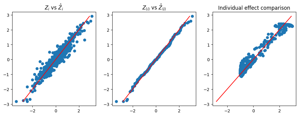
Figure 2 demonstrates the rationale underlying the Double-NN method. The left scatter plot compares the imputed and true values of the latent variables for a dataset simulated from (24), where the imputed values were collected at the last iteration of Algorithm 1. The comparison reveals a close match between the imputed and true latent variable values, with the variability of the imputed values representing the source of uncertainty in the data-generating system. This variability in the latent variables can be propagated to through the estimated inverse function , leading to the uncertainty in parameters and, consequently, the uncertainty in predictions. The middle scatter plot shows that the imputed latent variable values follows the standard Gaussian distribution, as expected. The right scatter plot compares the estimated and true values of the function , with the variability of the estimator representing its uncertainty. This plot further implies that the Double-NN method not only works for performing inference for the predictive ITE but also works for performing inference for CATE.
Example 2
Consider the data-generating equation
| (26) |
where with each element drawn independently from , and are generated as in Example 1 except that contains three extra false covariates, , , and . We simulated 20 datasets from this equation, each consisting of training samples and test samples.
For this example, we modeled both and using DNNs. Each of the DNNs consists of two hidden layers, each layer consisting of 10 hidden neurons. In consequence, has a total dimension of 363 .
Similar to Example 1, we also applied the CQR methods (Lei and Candès, 2021) to this example for comparison. The CQR methods were implemented as described in Example 1. The results were summarized in Table 3, which indicates again that the Double-NN method outperforms the CQR methods under all the three cases , , and . The prediction intervals resulting from the Double-NN method tend to be shorter, while their coverage rates tend to be closer to the nominal level.
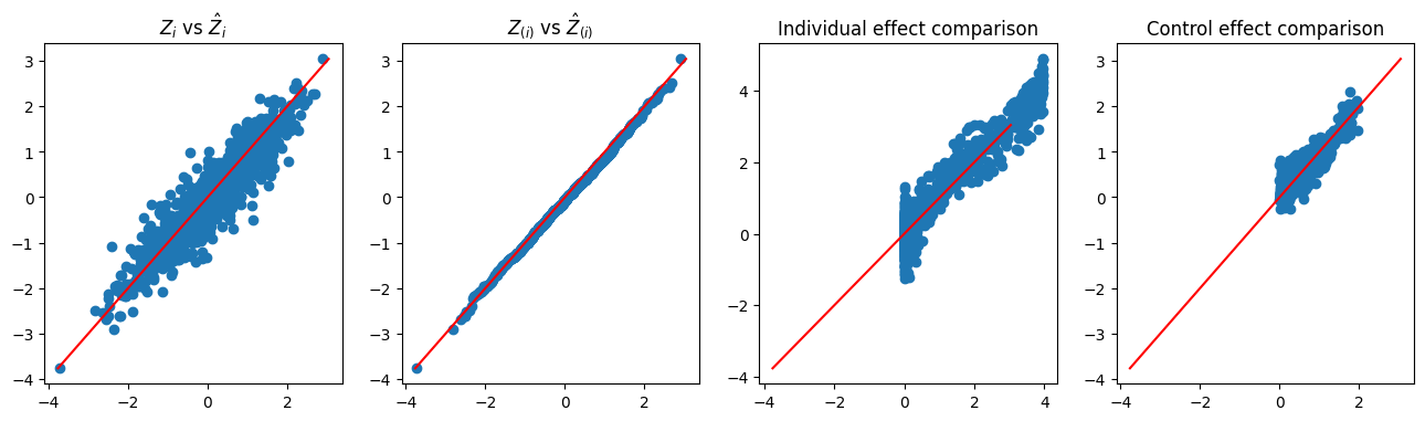
Similar to Figure 2, Figure 3 demonstrates the rationale underlying the Double-NN method, as well as its capability for CATE inference. The left plot demonstrates the variability embedded in the latent variables of the data-generating system. The middle-left plot shows that the imputed latent variables are distributed according to the standard Gaussian distribution, as expected. The right two plots display the estimates of and , respectively. Once again, we note that the variations of the estimates of and , as depicted in their respective scatter plots, reflect their uncertainty according to the theory of EFI.
Case Case Case Method Coverage Length Coverage Length Method Coverage Length Double-NN 0.9519 4.2727 0.9645 4.246 Double-NN 0.9604 6.0079 (0.0111) (0.0101) (0.0069) (0.0967) (0.0946) (0.1363) CQR-BART 0.9584 4.3586 0.9545 4.2658 CQR(inexact) 0.9386 6.0492 (0.0220) (0.4392) (0.0230) (0.4586) (0.0270) (0.6062) CQR-Boosting 0.9536 4.9942 0.9572 4.4393 CQR(exact) 0.9996 12.1252 (0.0175) (0.4044) (0.0194) (0.4213) (0.0007) (1.1022) CQR-RF 0.9563 5.6658 0.9580 4.4399 CQR(naive) 0.9988 11.5566 (0.0198) (0.4777) (0.0232) (0.5044) (0.0014) (0.9309) CQR-NN 0.9595 4.6748 0.9452 3.9579 (0.0165) (0.6015) (0.0185) (0.4301)
Precision in Estimation of Heterogeneous Effects
As demonstrated in Figure 2 and Figure 3, the Double-NN method can also be used for inference of CATE. The performance in CATE estimation is often measured using the expected Precision in Estimation of Heterogeneous Effects (PEHE), which is defined as:
where denotes the distribution function of the covariates . As we can see, summarizes the precision of the CATE over the entire sample space (Hill, 2011; Shalit et al., 2017; Caron et al., 2022). In practice, since we only observe the treatment effect on the treatment group, the target of interest is generally only for the treatment group, i.e , where denotes the distribution function of the covariates in the treatment group. We estimated by . For the Double-NN method, we set , where denotes the number of estimates of collected in a run of Algorithm 1.
For comparison, the existing CATE estimation methods, including single-learner (S-learner), two-learner (T-learner), and X-learner (Künzel et al., 2019), have been applied to the datasets generated above, where the RF and BART are used as the base learners. In the S-learner, a single outcome function is estimated using a base learner with all available covariates, where the treatment indicator is treated as a covariate, and then estimate CATE by , where denotes the outcome function estimator. The T-learner estimates the outcome functions using a base learner separately for the units under the control and those under the treatment, and then estimate CATE by , where denote the outcome function estimator for the assignment group . The X-learner builds on the T-learner; it uses the observed outcomes to estimate the unobserved ITEs, and then estimate the CATE in another step as if the ITEs were observed. Refer to Künzel et al. (2019) and Caron et al. (2022) for the detail. We implemented the S-learner, T-learner, and X-leaner using the package downloaded at https://github.com/albicaron/EstITE.
Table 4 compares the values of resulting from the Double-NN, S-learners, T-learners, and X-learners. for the models (24) and (26). The comparison shows that the Double-NN method outperforms the existing ones in achieving consistent CATE estimates over different covariate values. This is remarkable! As explained in Section 4, we would attribute this performance of the Double-NN method to its fidelity in parameter estimation (Liang et al., 2024). Compared to the MLE method, which serves as the prototype for the base learners, the Double-NN method is forced to be more robust to covariates due to added penalty term .
| Model (24) | Model (26) | ||||
| Method | Training | Test | Training | Test | |
| S-RF | 0.3769 0.0170 | 0.3660 0.0188 | 0.3722 0.0074 | 0.3377 0.0100 | |
| S-BART | 0.4233 0.0156 | 0.4344 0.0149 | 0.3371 0.0099 | 0.3418 0.0102 | |
| T-RF | 0.4545 0.0114 | 0.4198 0.0118 | 0.4095 0.0064 | 0.3488 0.0084 | |
| T-BART | 0.4190 0.0139 | 0.4236 0.0127 | 0.4308 0.0092 | 0.4298 0.0093 | |
| X-RF | 0.3416 0.0153 | 0.3451 0.0162 | 0.2761 0.0106 | 0.2789 0.0106 | |
| X-BART | 0.3863 0.0137 | 0.3972 0.0128 | 0.3853 0.0102 | 0.3862 0.0097 | |
| Double-NN | 0.2962 0.0167 | 0.3139 0.0178 | 0.3788 0.0105 | 0.3899 0.0110 | |
5.3 Real Data Analysis
5.3.1 Lalonde
The ‘LaLonde’ data is a well-known dataset used in causal inference to evaluate the effectiveness of a job training program in improving the employment prospects of participants. We used the dataset given in the package “twang” (Cefalu et al., 2021) among various versions. The dataset includes earning data in 1978 on 614 individuals, with 185 receiving job training and 429 in the control group. There are 8 covariates including various demographic, educational, and employment-related variables. While the LaLonde dataset has been widely used for ATE estimation, we use it to illustrate the Double-NN method for constructing ITE prediction intervals.
To evaluate the performance of different methods, we randomly split the LaLonde dataset into a training set and a test set. The training set, denoted by , consists of observations; while the test set, denoted by , consists of observations. We trained the Double-NN on and constructed prediction intervals for each subject in with a confidence level of . For the Double-NN, we modeled both and using DNNs. Each of the DNNs consists of two hidden layers, with each layer consisting of 10 hidden neurons. In consequence, has a dimension of 423 , a challenging task for uncertainty quantification of the model.
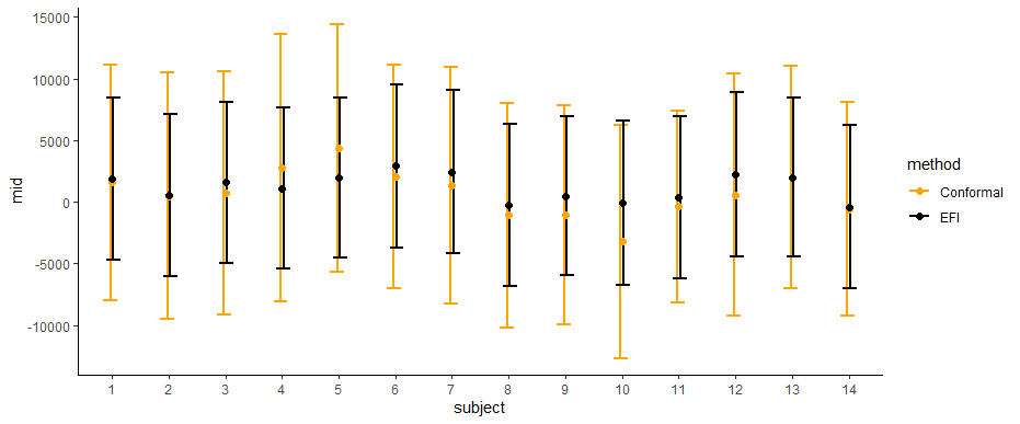
Figure 4 displays the constructed ITE prediction intervals for the test data, comparing the proposed method to the CQR method (Lei and Candès, 2021). The comparison shows that the prediction intervals resulting from the proposed method are shorter than those from the CQR method, while the centers of those intervals are similar. This suggests that the proposed method is able to estimate the ITEs with a higher degree of precision.
5.3.2 NLSM
This subsection conducts an analysis on the ‘National Study of Learning Mindsets’ (NLSM) dataset used in the 2018 Atlantic Causal Inference Conference workshop (Yeager et al., 2019; Carvalho et al., 2019). NSLM records the results of a randomized evaluation for a “nudge-like” intervention designed to instill students with a growth mindset. The dataset is available at https://github.com/grf-labs/grf/tree/master/experiments/acic18, which includes 10,391 students from 76 schools, with four student-level covariates and six school-level students. After factoring the categorical variables, the dimension of covariates increases to 29.
Due to unavailability of the true treatment effect values, we performed an exploratory analysis as in Lei and Candès (2021). In order to construct prediction intervals for the ITE, we split the dataset into two sets: and . The former has a sample size of , and the latter has a sample size of . For the Double-DNN method, we used DNNs to model the functions and . Each DNN consists of two hidden layers, with each hidden layer consisting of 10 hidden neurons. Therefore, the dimension of is 843 .
The Double-DNN was trained on and the prediction intervals were constructed on , which corresponds to case (iii) described in Section 5.1. This process was repeated 20 times. For comparison, the CQR method (Lei and Candès, 2021) was also applied to this example.
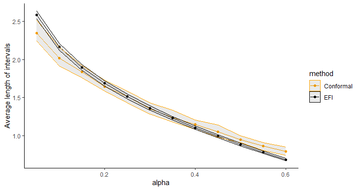 |
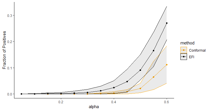
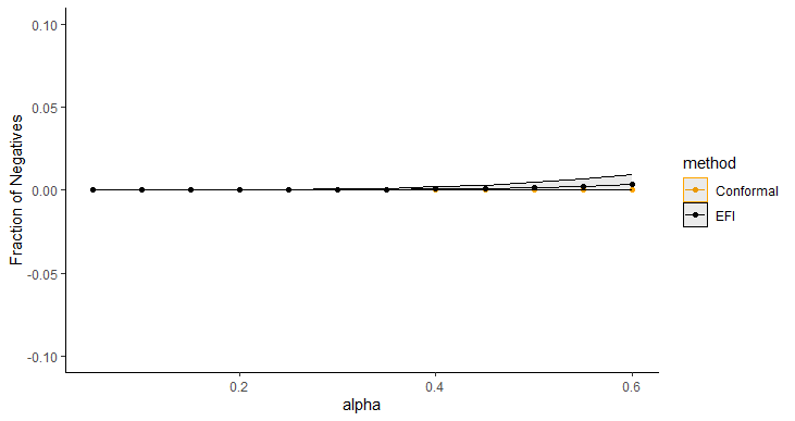
Figure 5 displays the average length of prediction intervals, obtained by Double-DNN and CQR, as a function of , with the upper and lower envelops being respectively the and quantiles across 20 runs. For this example, we implemented CQR using the “inexact” method, and therefore, its interval lengths tend to be short with approximate validity. However, as shown in Figure 5, the prediction intervals resulting from the Double-NN method tend to be even shorter than those from CQR as increases. Figure 6 (a) compares the fractions of the prediction intervals, obtained by Double-NN and CQR, that cover positive values only. While Figure 6 (b) compares the fractions of the prediction intervals that cover negative values only. In summary, the Double-NN can provide more accurate predictions for the ITE than CQR for this example. Specifically, the Double-NN identified fewer subjects with significant ITEs than the CQR, as implied by Figure 6 (a) and (b); while each has a narrow prediction interval, as implied by Figure 5.
| (a) | (b) |
|---|---|
 |
 |
6 Discussion
This paper extends EFI to statistical inference for large statistical models and applies the proposed Double-NN method to treatment effect estimation. The numerical results demonstrate that the Double-NN method significantly outperforms the existing CQR method in ITE prediction. As mentioned in the paper, we attribute the superior performance of the Double-NN method to its fidelity in parameter estimation. Due to the universal approximation ability of deep neural networks, the Double-NN method is generally applicable for causal effect estimation.
From the perspective of statistical inference, this paper advances the theory and methodology for making inference of large statistical models, allowing the model size to increase with the sample size at a rate of for any exponent . In particular, the Double-NN method provides a rigorous approach for quantifying the uncertainty of deep neural networks. In this paper, we have tested the performance of the Double-NN method on numerical examples with the exponent ranging , which all falls into the class of large models.
The Double-NN method can be further extended toward a general nonparametric approach for causal inference. Specifically, we can include an additional neural network to approximate the propensity score, enabling the outcome and propensity score functions to be simultaneously estimated. This extension will enable the use of inverse probability weighting methods to further improve ATE estimation, especially in the scenario where the covariate distributions in the treatment and control groups are imbalanced (Shalit et al., 2017; Hahn et al., 2020). From the perspective of EFI, this just corresponds to making inference for a different function. Similarly, for inference of ITE, a different function, including those adjusted with propensity scores, can also be used. The key advantage of EFI is its ability to automatically quantify the uncertainty of these functions as prescribed in (20), even when the functions are highly complex.
Regarding the size of large models, our theory does not preclude applications to large-scale DNNs with millions or even billions of parameters, as supported by the neural scaling law. As mentioned previously, Hestness et al. (2017) investigated the relationship between the DNN model size and the dataset size: they discovered a sub-linear scaling law of across various model architectures in machine learning applications, including machine translation, language modeling, image processing, and speech recognition. Their findings suggest that Theorem 3.1 remains valid for large-scale DNNs by choosing an appropriate growth rate for their depth.
In practice, we often encounter small--large- problems. For such a problem, we need to deal with a model of dimension , which is often termed as an over-parameterized model. A further extension of EFI for over-parameterized models is possible by imposing an appropriate sparsity constraint on . How to make post-selection inference with EFI for the over-parameterized models will be studied in future work.
Finally, we note that a recent work by Williams (2023) demonstrates how conformal prediction sets arise from a generalized fiducial distribution. Given the inherent connections between GFI and EFI, we believe that the results established in Williams (2023) should also apply to EFI. In particular, EFI follows the same switching principle as GFI (Hannig et al., 2016), which infers the uncertainty of the model parameters from the distribution of unobserved random errors. Further research on EFI from this perspective is of great interest, as it could potentially alleviate EFI’s reliance on assumptions about the underlying data distribution in prediction uncertainty quantification.
Availability
The code that implements the Double NN method can be found at https://github.com/sehwankimstat/DoubleNN.
Acknowledgments
Liang’s research is supported in part by the NSF grants DMS-2015498 and DMS-2210819, and the NIH grant R01-GM152717. The authors thank the editor, associate editor, and referee for their constructive comments, which have led to significant improvement of this paper.
Appendix: Supplement for “Extended Fiducial Inference for Individual Treatment Effects via Deep Neural Networks ”
Appendix 1 Theoretical Proofs
To prove the validity of the proposed method, it is sufficient to prove that constitutes a consistent estimator of , building on the theory developed in Liang et al. (2024). To ensure the self-contained nature of this paper, we provide a concise overview of the theory presented in Liang et al. (2024) in Section 1.1 of this supplement. Subsequently, our study will center on establishing the consistency of .
1.1 Outline of the Proof
First of all, we note that the theoretical study is conducted under the assumption that the EFI network has been correctly specified such that a sparse EFI network exists, from which the complete data can be generated, where represents the values of the latent variables realized in the observed samples. Specifically, we assume holds as .
For the EFI network, we define
| (S1) |
Therefore,
is the global maximizer of the posterior . Also, we define
| (S2) |
where is the log-normalizing constant of the posterior . Note that in the above derivation, can be ignored for simplicity since it is constant. For simplicity of notation, we let
be the Kullback-Leibler divergence between and . Regarding the EFI network, we make the following assumption:
Assumption 1
The EFI network satisfies the conditions:
-
(i)
The parameter space (of ) is convex and compact.
-
(ii)
for any , where denotes a generic sample as those in .
Define . By Assumption 1 and the weak law of large numbers,
| (S3) |
holds uniformly over the parameter space , where denotes convergence in probability. Further, we make the following assumption on , which is essentially an identifiability condition of .
Assumption 2
(i) is continuous in and is uniquely maximized at some point ; (ii) for any , the value exists, where , and .
Assumption 2 restricts the shape of around the global maximizer, which cannot be discontinuous or too flat. Given nonidentifiability of the neural network model, see e.g. Sun et al. (2022), we have implicitly assumed that each is unique up to loss-invariant transformations, e.g., reordering the hidden neurons within the same hidden layer or simultaneously altering the signs of certain weights and biases. The same assumption has often been used in theoretical studies of neural networks, see e.g. Liang et al. (2018b).
On the other hand, by Theorem 1 of Liang et al. (2018a), we have
| (S4) |
under some regularity conditions. Under Assumptions 1-2, Liang et al. (2024) proved the following lemma:
Lemma S1
For Lemma S1, the uniqueness of , up to some loss-invariant transformations as discussed previously, can be ensured by its consistency as established in the followed sections of this supplement, see equation (S20). The condition minimizing is generally implied by provided the consistency of , while the convergence of to a maximizer of is generally implied by the Monte Carlo nature of Algorithm 1. Therefore, by eq. (17) of the main text, if converges and converges to 0, we would have provided that the prior has been appropriately chosen such that is consistent for and is consistent for .
In summary, by Lemma S1, if we can choose an appropriate prior such that is consistent for , then is also consistent for and is consistent for . Establishing the consistency of will be the focus of Section 1.2 of this supplement. Note that showing the consistency of is relatively simpler than directly working on , as is based on the complete data.
Then, following from the consistency of , we immediately have
| (S5) |
As a slight relaxation for the definition of , we can write equation (7) of the main text as
| (S6) |
where is assumed to be known. By combining (S5) and (S6), we have
i.e., the EFI estimator is consistent for the inverse mapping . Further, by Slutsky’s theorem, the uncertainty of can be propagated to via the EFI estimator. Therefore, the extended fiducial density (EFD) function of can be approximated by
| (S7) |
where stands for the Dirac measure at a given point , , and for denotes random draws from the distribution under the limit setting of .
1.2 On the Consistency of under the Large Model Scenario
In this section, we first show that is consistent under the framework of imputation-regularized optimization (IRO) algorithm (Liang et al., 2018a) by assuming that the true values of are known and is subject to a mixture Gaussian prior. Subsequently, we show that is consistent.
1.2.1 An Auxiliary Stochastic Neural Network Model
To show is consistent, we introduce an auxiliary stochastic neural network (StoNet) model. For each of the hidden and output neurons of the model, we introduce a random noise:
| (S8) |
where indexes the layers of the DNN, and indexes the neurons at layer of the DNN, the random noise , denotes the weight on the connection from neuron of layer to neuron of layer , and denotes the activation function used for layer . Note that ’s are all known and pre-specified by the user, and represents the input layer. As a consequence of introducing the random noise, we can treat ’s as latent variables, where .
When considering a dataset of size , we let denote the latent variable imputed for neuron of layer for observation , let , and let denote the latent variables at layer for all observations. Recall that we have defined , , and . Given a set of pseudo-complete data , we define the posterior distribution of as:
| (S9) |
where with being the connection weights for layer ,
, , and represents a -dimensional multivariate Gaussian distribution.
Remark S1
It is interesting to point out that for the stochastic version of the EFI network, forms a directed cyclic graph (DCG): . See e.g. Sethuraman et al. (2023) for analysis of DCGs. For our case, is known, which serves as intervention variables and greatly simplifies the problem. Specifically, as , ’s can be uniquely determined via for a given set of and, therefore, (S9) is reduced to the posterior distribution for a conventional StoNet with serving as the input and serving as the target output.
Assumption 3
(i) The activation function used for each hidden neuron is -Lipschitz continuous for some constant ; (ii) for , where denotes the dimension of ; (iii) the network’s depth and widths ’s, for , are all allowed to increase with the sample size .
Assumption 3-(i) has covered many commonly used activation functions such as ReLU, tanh, and sigmoid. Assumption 3-(ii) restricts the width of the DNN. To model a dataset of dimension , we generally need a model of dimension . Since we do not aim to impose any sparsity constraints on in our main theory, we assume also satisfies the constraint such that is still possible to hold.
Suppose Assumption 1 and Assumption 3 hold. Following Liang et al. (2022b) and Sun and Liang (2022), we can establish the existence of a small value , as a function of , such that if and , then
| (S10) |
In other words, the DNN model in the EFI network and stochastic DNN model introduced above have asymptotically the same loss function as long as are sufficiently small and is sufficiently small.
1.2.2 Consistency of the Sparse DNN Model Estimation
This section gives a constructive proof for the consistency of based on the IRO algorithm (Liang et al., 2018a). To solve the optimization problem in (S11), the IRO algorithm starts with an initial weight setting and then iterates between the imputation and regularized-optimization steps:
-
•
Imputation: For each block, conditioned on the current parameter estimate , simulate the latent variables from the predictive distribution
(S13) where indexes iterations, , and denotes the component of corresponding to the weights at the -th layer.
-
•
Regularized-optimization: Given the pseudo-complete data , , , , update by maximizing the penalized log-likelihood function:
(S14) which, by the decomposition (S9), can be reduced to solving for , separately. The penalty function should be chosen such that forms a consistent estimator for the working true parameter
(S15) where the likelihood function of the latent variables is evaluated at , and corresponds to the true parameters of the underlying sparse DNN model.
To prove the consistency of as and approach to infinity, we need Assumptions 4-6 as specified below. For a matrix , we define the -sparse minimal eigenvalues as follows:
which represents the minimal eigenvalues of any -dimensional principal submatrix, and denotes the number of nonzero elements in . Let denote the sample covariance matrix of the input variables for the regression formed for neuron of layer at iteration , and let denote the size of the true regression model as implied by the working true parameter .
Assumption 4
(i) All the variables are uniformly bounded, where denotes the imputed values of at iteration ; (ii) there exist some constants and such that holds uniformly for any neuron and any iteration , where denotes the covariance matrix of .
Assumption 4-(i) restricts the pseudo-complete data to be uniformly bounded. To satisfy this condition, we can add a data transformation/normalization layer to the DNN model, ensuring that the transformed input values fall within the bounded set. Specifically, the transformation/normalization layer can form a bijective mapping and contain no tuning parameters. For example, when dealing with standard Gaussian random variables, we can transform them to be uniform over (0,1) via the probability integral transformation , the cumulative distribution function (CDF) of the standard Gaussian random variable.
Assumption 4-(ii) is natural for the problem. As implied by Assumption 3-(ii), the upper bound can always hold. For other layers, the upper bound is also true by Assumption 3-(ii), and the sparse eigenvalue property can be directly established, see Lemma S3 below.
Lemma S2
Consider a random matrix with . Suppose that the eigenvalues of are upper bounded, i.e., for some constant . Let denote an elementwise transformation of . Then
| (S16) |
for the tanh, sigmoid and ReLU transformations.
- Proof:
Lemma S3
Consider an auxiliary stochastic neural network as defined in (S8) with an activation function tanh, sigmoid, or ReLU. Then for any any layer , neuron , and iteration , there exists a number such that and hold.
-
Proof:
We use and to denote generic vectors corresponding to the -th layer, where . Additionally, we use and to denote the matrices (for all observations) corresponding to the -th layer. For the auxiliary stochastic neural network, since ’s have been set to very small values, it follows from (S8) that
where denotes elementwise product, , and . Then, for any ,
(S17) where , , denotes a diagonal matrix with the diagonal elements given by the vector .
By induction, building on Assumption 4-(i) and Lemma S2, we can assume that the maximum eigenvalue of is upper bounded by . By an extension of Ostrowski’s theorem, see Theorem 3.2 of Higham and Cheng (1998), we have
where the existence of the upper bound follows from the boundedness of as implied by Assumption 1-(i). By choosing as a one-hot vector, it is easy to see that for any ,
(S18) where denotes the th element of . This further implies, as ,
(S19) In words, has bounded mean and variance.
By Markov’s inequality, we can bound to a closed interval with a high probability, i.e., for some large constant . Therefore, for any activation function which has nonzero gradients on any closed interval, e.g., tanh and sigmoid, there exists a constant such that
which implies .
For the ReLU activation function, if a hidden neuron belongs to the true neuron set at iteration (as determined by ), then cannot be constantly 0 over all samples. Therefore, it is reasonable to assume that there exists a threshold such that for any true neuron in all iterations. Under this assumption, we would at least have
where denotes the set of true neurons at layer .
To study the property of the coefficient estimator for each regression formed in the auxiliary stochastic neural network, we introduce the following lemma, which is a restatement of Theorem 3.4 of Song and Liang (2023).
Lemma S4
(Theorem 3.4; Song and Liang (2023)) Consider a linear regression
where , , , , and is Gaussian noise. Suppose that the model satisfies the following conditions:
-
(A1)
(i) All the covariates are uniformly bounded; (ii) the dimensionality can be high with ; and (iii) there exists some integer (depending on and ) and a fixed constant such that and for any subset model , where denotes the size of the true model , and denotes the minimum eigenvalue of a square matrix. Let denote the MLE of the true model.
-
(A2)
(i) ; (ii) , where ’s and denote the true parameter values of the regression model, is a fixed constant, and is nondecreasing with respect to .
-
(A3)
Let each component of be subject to the following mixture Gaussian prior distribution
where , , and for some constant and sequence . Additionally, and for some sufficiently large .
Let denote the MAP estimator of . Then there exists a constant such that
Specifically, with dominating probability, we have if and 0 otherwise, where denotes the th element of , and denotes the element of that corresponds to .
It is easy to see that under Assumption 1, Assumption 3, and Assumption 4, each linear regression formed in the stochastic neural network satisfies conditions (A1) and (A2) of Lemma S4. In particular, we can set as the diameter of . To ensure the condition (A3) to be satisfied, we make the following assumption:
Assumption 5
Let each connection weight be subject to the following mixture Gaussian priro distribution:
where we set , and such that , , and for some constant and any . Additionally, there exists some constant such that .
It is easy to verify that the condition (A3) holds under Assumption 3-(ii) and Assumption 5. In addition, the -min condition, i.e., , is rather weak and can be generally satisfied as becomes large.
Theorem S1
-
Proof:
By the above analysis, each regression formed in the stochastic neural network satisfies the conditions of Lemma S4. Therefore, the sparse eigenvalue lower bounds established in Lemma S3 hold for the stochastic neural network. Further, by summarizing the -errors of coefficient estimation for all linear regressions, we can conclude the proof.
It is important to note that the condition allows the width of each layer of the neural network to increase with at a rate as high as . This accommodates the scenarios where for some . In this case, we have for the DNN model in the EFI network, which enables the uncertainty of to be properly quantified as implied by Theorem 3.1 proved below.
Further, let’s consider the mapping as defined in (S15), i.e.,
As argued in Liang et al. (2018a) and Nielsen (2000), it is reasonable to assume that the mapping is contractive. A recursive application of the mapping, i.e., setting , leads to a monotone increase of the target expectations
for .
Assumption 6
The mapping is differentiable. Let be the largest singular value of . There exists a number such that for all for sufficiently large and almost every training dataset .
Theorem S2
Suppose that a mixture Gaussian penalty is imposed on the weights of the DNN model in the EFI network; Assumptions 1 and 3-6 hold; is sufficiently small; and holds, where as defined in Section 1.2.1 and represents a constant. Then for sufficiently large and sufficiently large and almost every training dataset .
-
Proof:
This lemma directly follows from Theorem 4 of Liang et al. (2018a) that the estimator is consistent when both and are sufficiently large.
In summary, we have given a constructive proof for the consistency of sparse stochastic neural network based on the sparse learning theory developed for high-dimensional linear regression. Our proof implies that under the conditions of Theorem S2, such a consistent estimator can also be obtained by a direct calculation of as defined in (S11). Furthermore, it follows from (S12) that
| (S20) |
Proof of Theorem 3.1
- Proof:
In summary, through the introduction of an auxiliary stochastic neural network model and the utilization of the convergence theory of the IRO algorithm, we have justified the consistency of the sparse DNN model under mild conditions.
Remark S2
The result presented in Theorem 3.1 is interesting: we can set the width of each layer of the DNN model to be of order for some and set its depth to be for some . Given the approximation ability of the sparse DNN model as studied in Sun et al. (2022), where it was proven that a neural network of size for some has been large enough for approximating many classes of functions, EFI can be used for uncertainty quantification for deep neural networks if their sizes are appropriately chosen. Specifically, for the Double-NN approach, we can set the size of the first neural network (for approximation of the inverse function ) to be large under the constraint , and set the second neural network (for approximation of the function ) to be relatively small with the size for some . By the theory developed in this paper, the uncertainty of the second neural network can still be correctly quantified using EFI.
Appendix 2 CQR Method
For a test point belonging to the class , CQR aims to find the intervals and such that
Similarly, for a test point belonging to the class , CQR aims to find the intervals and such that
To achieve the above goals, CQR initially splits the training dataset to . A quantile regression model, such as BART or random forest, is trained on . Denote the output of the quantile regression by , and calculate the score for each . Note that acts like a residual derived from the validation set. Let . Then given below is the conformal prediction interval for any :
For a more refined approach, one can consider incorporating propensity scores as weights as discussed in Tibshirani et al. (2019).
Case (i) and Case (ii) described in Section 5.1 can be addressed by the above approach. However, for Case (iii) there, the conformal prediction needs further steps. First, construct a pair of prediction intervals at level ; namely, for and for . Then, construct an interval for ITE as follows:
We refer to this approach as the “naive” approach, which usually leads to very wide prediction intervals.
Another option for case (iii) is the so-called “nested” approach by splitting into two folds, denoted by . On the first fold, train and by applying conformal inference. On the second fold, for each , compute
where and are estimated based on . Note that the conformal inference is also applicable for the data with interval outcomes. Applying the conformal inference method with interval outcomes on for , yielding the interval . Applying the conformal inference twice results in a sparse utilization of data for training the regression model and, subsequently, wider prediction intervals. The inexact method involves fitting conditional quantiles of and , yielding an interval . The inexact method does not guarantee the coverage rate. Refer to Lei and Candès (2021) for the detail.
Appendix 3 Experimental Settings
To enforce a sparse DNN to be learned for the inverse function , we impose the following mixture Gaussian prior on each element of :
| (S21) |
where represents a generic element of and, unless stated otherwise, we set , and . The elements of are a priori independent.
For EFI, we employ SGHMC in latent variable sampling, i.e., we simulate in the following formula:
where , is the momentum parameter, , and is the learning rate. It is worth noting that the algorithm is reduced to SGLD if we set .
In the simulations, we set the learning rate sequence and the step size sequence in the forms:
for some constants , , and , and . The values of , , , and used in different experiments are given below.
3.1 ATE
From the point of view of equation solving, the model (22) in the main text can also be written as
| (S22) |
where , , and . Let . Equation (S22) can be solved under the standard framework of EFI. Unless otherwise noted, all results in this paper are based on solving this type of transformed equations.
We set and . For , we set 200000, 1000000, 54000, 1000000). For and 1000, we set , 54000, 1000000).
We set as the number of burn-in iterations, and set as the number of iterations used for fiducial sample collection. We thinned the Markov chain by a factor of ; that is, we collected samples in each run.
We set and in construction of the energy function, and perform gradient clipping by norm with 5000 during the first 100 iterations (for finding a reasonably good initial point).
The DNN in the EFI network has two hidden layers, with the widths given by and , respectively.
3.2 Linear control response with Non-linear treatment response
We set , , and and for and for all other parameters. Refer to Figure S1 for the definition of .
For initialization, we update the with randomly sampled for the first 5000 iterations. We set as the number of burn-in iterations, and set as the number of iterations used for fiducial sample collection. We thinned the Markov chain by a factor of ; that is, we collected samples in each run. We set and in construction of the energy function, and perform gradient clipping by norm with 5000 during the first 100 iterations.
The DNN in the EFI network has two hidden layers, with the widths given by and , respectively. The DNN used for modeling the treatment effect has two hidden layers, each hidden layer consisting of 10 hidden neurons.
3.3 Non-linear control response with Non-linear treatment response
We set , , and and for and , and set for all other parameters. Refer to Figure S1 for the definitions of and .
For initialization, we update the with randomly sampled for the first 5000 iterations. We set as the number of burn-in iterations, and set as the number of iterations used for fiducial sample collection. We thinned the Markov chain by a factor of ; that is, we collected samples in each run. We set and in construction of the energy function, and perform gradient clipping by norm with 5000 during the first 100 iterations.
The DNN in the EFI network has two hidden layers, with the widths given by and , respectively. The DNN used for modeling the treatment effect has two hidden layers, each hidden layer consisting of 10 hidden neurons. The DNN used for modeling the response function under the control has two hidden layers, each hidden layer consisting of 10 hidden neurons.
3.4 Lalonde
We set , , and and for and , and for all other parameters. Refer to Figure S1 for the definitions of and .
For initialization, we update the with randomly sampled for the first 10,000 iterations. We set as the number of burn-in iterations and set as the number of iterations used for fiducial sample collection. We thinned the Markov chain by a factor of ; that is, we collected samples in each run. We set and in construction of the energy function, and perform gradient clipping by norm with 5000 for first 100 iterations.
The DNN in the EFI network has two hidden layers, with the widths given by and , respectively. The DNN used for modeling the treatment effect contains two hidden layers, each hidden layer containing 10 hidden neurons. The DNN used for modeling the response function under the control contains two hidden layers, each hidden layer containing 10 hidden neurons.
3.5 NLSM
We set , , and and for and , and for all other parameters. Refer to Figure S1 for the definitions of and .
For initialization, we update the with randomly sampled for the first 10,000 iterations. We set as the number of burn-in iterations and set as the number of iterations used for fiducial sample collection. We thinned the Markov chain by a factor of ; that is, we collected samples in each run. We set and in construction of the energy function, and perform gradient clipping by norm with 5000 for first 100 iterations.
The DNN in the EFI network contains two hidden layers, with the widths given by and , respectively. The DNN used for modeling the treatment effect contains two hidden layers, each hidden layer containing 10 hidden neurons. The DNN used for modeling the response function under control contains two hidden layers, each hidden layer containing 10 hidden neurons.
References
- Bang and Robins (2005) Bang, H. and Robins, J. M. (2005), “Doubly Robust Estimation in Missing Data and Causal Inference Models,” Biometrics, 61, 962–972.
- Bolcskei et al. (2019) Bolcskei, H., Grohs, P., Kutyniok, G., and Petersen, P. (2019), “Optimal approximation with sparsely connected deep neural networks,” SIAM Journal on Mathematics of Data Science, 1, 8–45.
- Breiman (1998) Breiman, L. (1998), “Arcing classifier (with discussion and a rejoinder by the author),” Annals of Statistics, 26, 801–849.
- Breiman (2001) — (2001), “Random forests,” Machine learning, 45, 5–32.
- Caron et al. (2022) Caron, A., Baio, G., and Manolopoulou, I. (2022), “Estimating Individual Treatment Effects using Non-Parametric Regression Models: a Review,” Journal of the Royal Statistical Society Series A: Statistics in Society, 185, 1115–1149.
- Carvalho et al. (2019) Carvalho, C. M., Feller, A., Murray, J., Woody, S., and Yeager, D. S. (2019), “Assessing Treatment Effect Variation in Observational Studies: Results from a Data Challenge,” Observational Studies.
- Cefalu et al. (2021) Cefalu, M., Ridgeway, G., McCaffrey, D., Morral, A., Griffin, B. A., and Burgette, L. (2021), “Package ‘twang’: Toolkit for Weighting and Analysis of Nonequivalent Groups,” R Package.
- Chen et al. (2014) Chen, T., Fox, E., and Guestrin, C. (2014), “Stochastic gradient hamiltonian monte carlo,” in International conference on machine learning, pp. 1683–1691.
- Chipman et al. (2010) Chipman, H. A., George, E. I., and McCulloch, R. E. (2010), “BART: Bayesian Additive Regression Trees,” The Annals of Applied Statistics, 4, 266–298.
- Deng et al. (2019) Deng, W., Zhang, X., Liang, F., and Lin, G. (2019), “An adaptive empirical Bayesian method for sparse deep learning,” Advances in neural information processing systems, 32.
- Dittmer et al. (2018) Dittmer, S., King, E. J., and Maass, P. (2018), “Singular Values for ReLU Layers,” IEEE Transactions on Neural Networks and Learning Systems, 31, 3594–3605.
- Dorie and Hill (2020) Dorie, V. and Hill, J. L. (2020), “Bartcause: Causal Inference using Bayesian Additive Regression Trees [R package bartCause version 1.0-4],” R Package.
- Farrell et al. (2021) Farrell, M., Liang, T., and Misra, S. (2021), “Deep Neural Networks for Estimation and Inference,” Econometrica, 89, 181–213.
- Fisher (1935) Fisher, R. A. (1935), “The fiducial argument in statistical inference,” Annals of Eugenics, 6, 391–398.
- Foster et al. (2011) Foster, J. C., Taylor, J. M., and Ruberg, S. J. (2011), “Subgroup identification from randomized clinical trial data,” Statistics in Medicine, 30.
- Fraser (1966) Fraser, D. A. S. (1966), “Structural probability and a generalization,” Biometrika, 53, 1–9.
- Fraser (1968) — (1968), The Structure of Inference, New York-London-Sydney: John Wiley & Sons.
- Guan and Yang (2019) Guan, Q. and Yang, S. (2019), “A Unified Framework for Causal Inference with Multiple Imputation Using Martingale,” arXiv: Methodology.
- Hahn et al. (2020) Hahn, P. R., Murray, J. S., and Carvalho, C. M. (2020), “Bayesian Regression Tree Models for Causal Inference: Regularization, Confounding, and Heterogeneous Effects (with Discussion),” Bayesian Analysis, 15, 965 – 2020.
- Hannig (2009) Hannig, J. (2009), “On generalized fiducial inference,” Statistica Sinica, 19, 491–544.
- Hannig et al. (2016) Hannig, J., Iyer, H., Lai, R. C. S., and Lee, T. C. M. (2016), “Generalized Fiducial Inference: A Review and New Results,” Journal of the American Statistical Association, 111, 1346–1361.
- Hestness et al. (2017) Hestness, J., Narang, S., Ardalani, N., Diamos, G. F., Jun, H., Kianinejad, H., Patwary, M. M. A., Yang, Y., and Zhou, Y. (2017), “Deep Learning Scaling is Predictable, Empirically,” ArXiv, abs/1712.00409.
- Higham and Cheng (1998) Higham, N. J. and Cheng, S. H. (1998), “Modifying the inertia of matrices arising in optimization,” Linear Algebra and its Applications, 261–279.
- Hill (2011) Hill, J. L. (2011), “Bayesian Nonparametric Modeling for Causal Inference,” Journal of Computational and Graphical Statistics, 20, 217–240.
- Hornik (1991) Hornik, K. (1991), “Approximation capabilities of multilayer feedforward networks,” Neural Networks, 4, 251–257.
- Hornik et al. (1989) Hornik, K., Stinchcombe, M., and White, H. (1989), “Multilayer feedforward networks are universal approximators,” Neural Networks, 2, 359–366.
- Imbens (2004) Imbens, G. (2004), “Nonparametric Estimation of Average Treatment Effects Under Exogeneity: A Review,” The Review of Economics and Statistics, 86, 4–29.
- Imbens and Rubin (2015) Imbens, G. W. and Rubin, D. B. (2015), Causal Inference for Statistics, Social, and Biomedical Sciences: An Introduction, USA: Cambridge University Press.
- Javanmard and Montanari (2014) Javanmard, A. and Montanari, A. (2014), “Confidence iReferntervals and hypothesis testing for high-dimensional regression,” Journal of Machine Learning Research, 15, 2869–2909.
- Jiang (2007) Jiang, W. (2007), “Bayesian variable selection for high dimensional generalized linear models: convergence rates of the fitted densities,” The Annals of Statistics, 35, 1487–1511.
- Kidger and Lyons (2020) Kidger, P. and Lyons, T. (2020), “Universal Approximation with Deep Narrow Networks,” Proceedings of Machine Learning Research, 125, 1–22.
- Kim et al. (2023) Kim, N., Min, C., and Park, S. (2023), “Minimum width for universal approximation using ReLU networks on compact domain,” ArXiv, abs/2309.10402.
- Künzel et al. (2019) Künzel, S. R., Sekhon, J. S., Bickel, P. J., and Yu, B. (2019), “Metalearners for estimating heterogeneous treatment effects using machine learning,” Proceedings of the National Academy of Sciences of the United States of America, 116, 4156 – 4165.
- Lee et al. (2016) Lee, J., Sun, D., Sun, Y., and Taylor, J. (2016), “Exact post-selection inference, with application to the Lasso,” Annals of Statistics, 44, 907–927.
- Lei and Candès (2021) Lei, L. and Candès, E. J. (2021), “Conformal Inference of Counterfactuals and Individual Treatment Effects,” Journal of the Royal Statistical Society Series B: Statistical Methodology, 83, 911–938.
- Liang et al. (2018a) Liang, F., Jia, B., Xue, J., Li, Q., and Luo, Y. (2018a), “An imputation–regularized optimization algorithm for high dimensional missing data problems and beyond,” Journal of the Royal Statistical Society, Series B, 80, 899–926.
- Liang et al. (2024) Liang, F., Kim, S., and Sun, Y. (2024), “Exended Fiducial Inference: Toward an Automated Process of Statistical Inference,” Journal of the Royal Statistical Society, Series B, in press.
- Liang et al. (2018b) Liang, F., Li, Q., and Zhou, L. (2018b), “Bayesian Neural Networks for Selection of Drug Sensitive Genes,” Journal of the American Statistical Association, 113, 955–972.
- Liang et al. (2022a) Liang, F., Xue, J., and Jia, B. (2022a), “Markov neighborhood regression for high-dimensional inference,” Journal of the American Statistical Association, 117, 1200–1214.
- Liang et al. (2022b) Liang, S., Sun, Y., and Liang, F. (2022b), “Nonlinear Sufficient Dimension Reduction with a Stochastic Neural Network,” NeurIPS 2022.
- Lu et al. (2018) Lu, M., Sadiq, S., Feaster, D. J., and Ishwaran, H. (2018), “Estimating Individual Treatment Effect in Observational Data Using Random Forest Methods,” Journal of Computational and Graphical Statistics, 27, 209 – 219.
- Martin (2023) Martin, R. (2023), “Fiducial inference viewed through a possibility-theoretic inferential model lens,” Journal of Machine Learning Research, 215, 299–310.
- Murph et al. (2022) Murph, A. C., Hannig, J., and Williams, J. P. (2022), “Generalized Fiducial Inference on Differentiable Manifolds,” arXiv:2209.15473.
- Nielsen (2000) Nielsen, S. (2000), “The stochastic EM algorithm: Estimation and asymptotic results,” Bernoulli, 6, 457–489.
- Park et al. (2020) Park, S., Yun, C., Lee, J., and Shin, J. (2020), “Minimum Width for Universal Approximation,” ArXiv, abs/2006.08859.
- Petersen and Voigtlaender (2018) Petersen, P. and Voigtlaender, F. (2018), “Optimal approximation of piecewise smooth functions using deep ReLU neural networks,” Neural Networks, 108, 296–330.
- Portnoy (1986) Portnoy, S. (1986), “On the central limit theorem in when ,” Probability Theory and Related Fields, 73, 571–583.
- Portnoy (1988) — (1988), “Asymptotic behavior of likelihood methods for exponential families when the number of parameters tend to infinity,” Annals of Statistics, 16, 356–366.
- Robbins and Monro (1951) Robbins, H. and Monro, S. (1951), “A Stochastic Approximation Method,” Annals of Mathematical Statistics, 22, 400–407.
- Robins et al. (1994) Robins, J. M., Rotnitsky, A., and Zhao, L. P. (1994), “Estimation of regression coefficients when some regressors are not always observed,” Journal of the American Statistical Association, 89, 846–866.
- Romano et al. (2019) Romano, Y., Patterson, E., and Candès, E. J. (2019), “Conformalized Quantile Regression,” in Neural Information Processing Systems.
- Rosenbaum (1987) Rosenbaum, P. R. (1987), “Model-Based Direct Adjustment,” Journal of the American Statistical Association, 82, 387–394.
- Rosenbaum (2002) — (2002), Observational Studies (2nd edition), New York: Springer.
- Rubin (1974) Rubin, D. B. (1974), “Estimating causal effects of treatments in randomized and nonrandomized studies.” Journal of Educational Psychology, 66, 688–701.
- Schapire (1990) Schapire, R. E. (1990), “The Strength of Weak Learnability,” Machine Learning, 5, 197–227.
- Schmidt-Hieber (2020) Schmidt-Hieber, J. (2020), “Nonparametric regression using deep neural networks with ReLU activation function,” The Annals of Statistics, 48, 1875–1897.
- Sethuraman et al. (2023) Sethuraman, M. G., Lopez, R., Mohan, R. V., Fekri, F., Biancalani, T., and Hutter, J.-C. (2023), “NODAGS-Flow: Nonlinear Cyclic Causal Structure Learning,” in International Conference on Artificial Intelligence and Statistics.
- Shafer and Vovk (2008) Shafer, G. and Vovk, V. (2008), “A Tutorial on Conformal Prediction,” J. Mach. Learn. Res., 9, 371–421.
- Shalit et al. (2017) Shalit, U., Johansson, F. D., and Sontag, D. A. (2017), “Estimating individual treatment effect: generalization bounds and algorithms,” in Proceedings of the 34th International Conference on Machine Learning, PMLR, pp. 3076–3085.
- Song and Liang (2023) Song, Q. and Liang, F. (2023), “Nearly optimal Bayesian Shrinkage for high dimensional regression,” China Science Mathematics, 66, 409–442.
- Song et al. (2020) Song, Q., Sun, Y., Ye, M., and Liang, F. (2020), “Extended Stochastic Gradient MCMC for Large-Scale Bayesian Variable Selection,” Biometrika, 107, 997–1004.
- Sun and Liang (2022) Sun, Y. and Liang, F. (2022), “A kernel-expanded stochastic neural network,” Journal of the Royal Statistical Society Series B, 84, 547–578.
- Sun et al. (2022) Sun, Y., Song, Q., and Liang, F. (2022), “Consistent Sparse Deep Learning: Theory and Computation,” Journal of the American Statistical Association, 117, 1981–1995.
- Tibshirani et al. (2019) Tibshirani, R. J., Foygel Barber, R., Candes, E., and Ramdas, A. (2019), “Conformal Prediction Under Covariate Shift,” in Advances in Neural Information Processing Systems, eds. Wallach, H., Larochelle, H., Beygelzimer, A., d'Alché-Buc, F., Fox, E., and Garnett, R., Curran Associates, Inc., vol. 32.
- van de Geer et al. (2014) van de Geer, S., Bühlmann, P., Ritov, Y., and Dezeure, R. (2014), “On asymptotically optimal confidence regions and tests for high-dimensional models,” Ann. Statist., 42, 1166–1202.
- Vovk et al. (2005) Vovk, V., Gammerman, A., and Shafer, G. (2005), Algorithmic Learning in a Random World, Springer.
- Wager and Athey (2018) Wager, S. and Athey, S. (2018), “Estimation and Inference of Heterogeneous Treatment Effects using Random Forests,” Journal of the American Statistical Association, 113, 1228–1242.
- Williams (2023) Williams, J. P. (2023), “Model-free generalized fiducial inference,” .
- Yeager et al. (2019) Yeager, D. S., Hanselman, P., Walton, G. M., Murray, J. S., Crosnoe, R., Muller, C., Tipton, E., Schneider, B., Hulleman, C. S., Hinojosa, C. P., Paunesku, D., Romero, C., Flint, K., Roberts, A., Trott, J., Iachan, R., Buontempo, J., Yang, S. M., Carvalho, C. M., Hahn, P. R., Gopalan, M., Mhatre, P., Ferguson, R., Duckworth, A. L., and Dweck, C. S. (2019), “A national experiment reveals where a growth mindset improves achievement,” Nature, 573.
- Zabell (1992) Zabell, S. L. (1992), “R. A. Fisher and Fiducial Argument,” Statistical Science, 7, 369–387.
- Zetterqvist and Sjölander (2015) Zetterqvist, J. and Sjölander, A. (2015), “Doubly Robust Estimation with the R Package drgee,” Epidemiologic Methods, 4, 69–86.
- Zhang and Zhang (2014) Zhang, C.-H. and Zhang, S. S. (2014), “Confidence intervals for low dimensional parameters in high dimensional linear models,” Journal of the Royal Statistical Society: Series B (Statistical Methodology), 76, 217–242.