Extended Gini-type measures of risk and variability
Abstract
The aim of this paper is to introduce a risk measure that extends the Gini-type measures of risk and variability, the Extended Gini Shortfall, by taking risk aversion into consideration. Our risk measure is coherent and catches variability, an important concept for risk management. The analysis is made under the Choquet integral representations framework. We expose results for analytic computation under well-known distribution functions. Furthermore, we provide a practical application.
JEL classification: C6, G10
keywords:
risk measures, variability measures, risk aversion, signed Choquet integral, Extended Gini Shortfall.1 Introduction
In modern risk management, a large number of risk measures have been proposed in the literature. These measures are mappings from a set of random variables (financial losses) to real numbers. At first, the focus were on the variability over an expected return, as is the case for the well-known variance. After the collapses and crises in financial systems, a prominent trend associated with tail-based risk measures has emerged, especially with the most popular ones nowadays: the Value-at-Risk (VaR) and the Expected Shortfall (ES). However, this kind of risk measures does not capture the variability of a financial position, a primitive but relevant concept. In order to solution this issue, some authors have proposed and studied specific examples of risk measures.
In this sense, Fischer [8] considered combining the mean and semi-deviations. Regarding tail risk, Furman and Landsman [10] proposed a measure that weighs the mean and standard deviation in the truncated tail by VaR, while Righi and Ceretta [17] considered penalizing the ES by the dispersion of losses exceeding it. From a practical perspective, Righi and Borenstein [18] explored this concept, calling the approach as loss-deviation, for portfolio optimization. In a more general fashion, Righi [19] presents results and examples about compositions of risk and variability measures in order to ensure solid theoretical properties.
Recently, Furman et al. [11] introduced the Gini Shortfall (GS) risk measure which is coherent and satisfies co-monotonic additivity. GS is a composition between ES and tail based Gini coefficient. However, GS supposes that all individuals have the same attitude towards risk, while agents differ in the way they take personal decisions that involve risk because of discrepancies in their risk aversion. To incorporate such psychological behavior in tail risk analysis, we introduce a generalized version of the GS. This risk measure, called Extended Gini Shortfall (EGS), captures the notion of variability, satisfies the co-monotonic additivity property, and it is coherent under a necessary and sufficient condition for its loading parameter. The consideration of the decision-maker risk aversion, joined to these properties, is in consonance to what agents seek when searching for a suitable measure of risk. The approach followed in this article leads us to a new family of spectral risk measures, proposed by Acerbi [1], with an attractive weighting function.
In this sense, we discuss, in a separated manner, the properties from the variability term and our composed risk measure. Moreover, we discuss in details the role of each parameter in the mentioned weighting function. Furthermore, we expose results on analytic formulations for computation of EGS under known distribution functions. Our focus in this paper is on theoretical results, but this approach gives rise to further forthcoming investigations. In this sense, risk forecasting of our new family of risk measures is a subject that deserves a further and separate survey which will be made in a forthcoming work.
The rest of the paper is organized as follows. In Section 2, we present and discuss some preliminaries such as essential properties of measures of risk and variability, as well we elucidate the role of the signed Choquet integral. In section 3, we start with the Classical and Extended Gini functionals in order to introduce the concept and explore properties about what we call Tail Extended Gini functional and Extended Gini Shortfall. In Section 4, we give the closed-form of our risk measures class for elliptical distributions and then derive the uniform, Normal and Student-t cases. Section 5 illustrates an application of the introduced risk measures class in practice.
2 Preliminaries
We first introduce some basic notation. Let be an atomless probability space. All equations and inequalities are in the almost surely sense. Let , , denote the set of all random variables (rv’s from now on) in with finite q-th moment and be the set of all essentially bounded rv’s. Throughout this paper, is a rv modeling financial losses (profits) when it has positive (negative) values. For every denotes the cdf of , and denote any uniform rv such that the equation holds. The existence of such rv’s is assured in Rüschendorf ([21], Proposition 1.3). We denote as the p-quantile of . Two rv’s and are co-monotonic when . Throughout the present paper, we deal with several convex cones of rv’s, of which is of particular importance and is always contained in .
We begin by exposing definitions of both risk and variability measures. We assume throughout the paper that all functionals respect the following property, which is essential in order to obtain a functional directly from its distribution function.
Definition 2.1.
A functional is said to be law invariant if it fulfills the following property:
(A) Law Invariance: If and have the same distributions under , succinctly , then .
Definition 2.2.
A risk measure is a functional , which may fulfills the following properties:
(B1) Monotonicity: when are such that -almost surely.
(B2) Translation invariance: for all and .
(A1) Positive homogeneity: for all and .
(A2) Subadditivity: for all .
(A3) Co-monotonic additivity: for every co-monotonic pair .
A risk measure is monetary if it satisfies properties (B1) and (B2), and it is coherent if it satisfies furthermore (A1) and (A2).
Remark 2.3.
Definition 2.4.
A functional is a measure of variability, which may fulfills the following properties222Inspired from the deviation measures notion of Rockafellar et al. [20].:
(C1) Standardization: for all .
(C2) Location invariance: for all and .
(A1) Positive homogeneity: for all and .
(A2) Subadditivity: for all
(A3) Co-monotonic additivity: for every co-monotonic pair .
A measure of variability is coherent if it further satisfies (C1), (C2), (A1) and (A2).
Remark 2.5.
For instance, the most classical measures of variability are the Variance and the Standard Deviation. The variance functional satisfies properties (A), (C1), (C2) but not (A1) or (A2), hence it is not coherent. On the other side, the standard deviation functional, since satisfying all aforementioned properties, is coherent. Neither the variance nor the standard deviation is co-monotonically additive.
The notion of signed Choquet integral plays a pivotal role thereafter. It originates from Choquet [4], in the framework of capacities, and is further characterized and studied in decision theory by Schmeidler ([22], [23]).
Definition 2.6.
A function is called a distortion function when it is non-decreasing and satisfies the boundary conditions and . Let be a distortion function, the functional defined by the equation:
| (2.1) |
for all is called the (increasing) Choquet integral. Whenever is of finite variation, is called the signed Choquet integral.
Remark 2.7.
Remark 2.8.
The signed Choquet integral is co-monotonically additive, as we can readily see from representation (2.2) (cf. Schmeidler [22]). Moreover we know from Yaari [26] and Föllmer and Schied ([9], Theorem 4.88), that any law-invariant risk measure is co-monotonically additive and monetary if and only if it can be represented as a Choquet integral. Furthermore, the functional is sub-additive if and only if the function is convex (cf. Yaari [26] and Acerbi [1]). Moreover, as proved in Furman et al. [11], regarding the weighting functional , the integral is monotone if and only if on and it is sub-additive if and only if is non-decreasing on . The major difference between a (an increasing) Choquet integral and a signed one is that the latter, being more general, is not necessarily monotone.
One of the practical and theoretical reasons for what we are particularly interested in signed Choquet integral is that we know that a suitable risk measure should be monotone as argued by Artzner et al. [2], but this issue is irrelevant for a measure of variability. In other words, signed Choquet integral is relevant as long as a measure of variability is concerned. The following theorem is enunciated with a complete proof in Furman et al. [11], it gives the characterization for co-monotonically additive and coherent measures of variability.
Theorem 2.9.
Let be any -continuous functional. The following three statements are equivalent:
(i) is a co-monotonically additive and coherent measure of variability.
(ii) There is a convex function , such that
| (2.4) |
(iii) There is a non-decreasing function such that
| (2.5) |
Next, we recall a few partial orders of variability that have been popular in economics, insurance, finance and probability theory:
Definition 2.10.
For , is second-order stochastically dominated (SSD) by , succinctly , if for all increasing convex functions .
If in addition, , then we say that is smaller than in convex order, succinctly .333 We say equally is a Mean Preserving Spread of , succinctly .
Under this framework we have the following properties for risk and variability measures:
(B3) SSD-monotonicity: if , then .
(C3) CX-monotonicity: if , then .
3 Extended Gini Shortfall
In this section, we expose our main contribution, which is based on the Gini coefficient, a free-center measure of variability that was introduced by Corrado Gini as an alternative to the variance measure (e.g., Giorgi ([12], [13]) and Ceriani and Verme [3]). The Gini coefficient has been remarkably influential in numerous research areas (e.g, Yitzhaki and Schechtman [30] and the references therein). Yitzhaki [28] lists more than a dozen alternative presentations of the Gini coefficient. We now present a formal definition.
Definition 3.1.
The Gini coefficient is a functional defined conform:
| (3.1) |
where and are two independent copies of .
Remark 3.2.
The Gini coefficient can be written in terms of a signed Choquet integral:
| (3.2) |
From Theorem 2.9, it follows immediately that the Gini coefficient is a coherent measure of variability and it is CX-monotone. Moreover, equation (3.2) can be written in terms of covariance (which is the most common formula of the Gini coefficient):
| (3.3) |
We recall that can be any uniformly on distributed rv, and is a uniform rv such that the equation holds.
The Gini functional supposes that all individuals have the same attitude towards risk. Nonetheless, the concept can be extended into a family of measures of variability differing from each other in the decision-maker’s degree of risk aversion, which is reflected in this paper by the parameter . The basic definition of the Extended Gini coefficient is based on the covariance term. We refer to Yitzhaki [27], Shalit and Yitzhaki [24], Yitzhaki and Schechtman [29], and Yitzhaki and Schechtman [30] for an overview of the Extended Gini properties. We now expose it in a formal sense.
Definition 3.3.
The Extended Gini coefficient is a functional defined conform:
| (3.4) |
Remark 3.4.
There are special cases of interest for the Extended Gini:
-
For : the Extended Gini coefficient becomes the simple Gini.
-
For : the Extended Gini reflects the attitude of a max-min investor who expresses risk only in terms of the worst outcome.
-
For : the Extended Gini tends to zero and represents the attitude of a risk-neutral individual who does not care about variability.
We now explore the characterization of the Extended Gini coefficient as a signed Choquet integral. In this sense, note that from equation (2.5) in Theorem 2.9, if one sets for and , we run into . With that in mind, we now state and prove the formal result.
Proposition 3.5.
The Extended Gini functional is a CX-monotone coherent measure of variability, represented by the signed Choquet integral
| (3.5) |
Proof.
We recall that can be any uniformly distributed rv on such that the equation holds, where . In order to obtain the proof, we need the claim that for , and . In order to prove it, we get that
Under this perspective, we can easily verify that: . Thus, we get the following:
From this signed Choquet integral representation, the other claims in the proposition follow immediately from Theorem 2.9 and the fact that all coherent measures of variability are CX-monotone. This concludes the proof. ∎
Based on the exposed content, we now turn the focus to an adaptation to the tails of the distribution function. In this sense, we now introduce the Tail Extended Gini (TEG) functional, as well formally prove its properties and Choquet integral representation.
Definition 3.7.
The Tail Extended Gini is a functional defined conform:
| (3.7) |
Proposition 3.8.
The Tail Extended Gini is standardized, location invariant, positively homogeneous and co-monotonic additive. Moreover, it is a signed Choquet integral conform:
| (3.8) |
Proof.
The fact that the Tail Extended Gini is standardized, location invariant, positively homogeneous is easily realized from its definition. For the Choquet representation, we again recall that can be any uniformly distributed rv on such that the equation holds, where . Thus, we obtain that
In fact, from the proof of the previous proposition we have that . Finally, the Choquet representation implies co-monotonic additivity. This completes the proof. ∎
Remark 3.9.
However, as shown in a counter example (for ) by Furman et al. [11], the Tail Extended Gini is not sub-additive. Therefore, unlike the Extended Gini functional, the tail counterpart is not a coherent measure of variability.
Despite the fact that TEG is not a coherent measure of variability, we will show now that a linear combination of the Expected Shortfall with the Tail Extended Gini gives rise to a coherent risk measure, the Extended Gini Shortfall, that quantifies both the magnitude and the variability of tail risks. We now define such a combination.
Definition 3.10.
Let . We have that the Value at Risk and the Expected Shortfall are functionals and defined conform:
| (3.9) |
| (3.10) |
Remark 3.11.
It is a well-established fact that ES is a SSD-monotone comonotonic additive coherent risk measure. When the cdf is continuous, ES coincides with tail conditional expectation .
Definition 3.12.
The Extended Gini Shortfall is a functional defined conform:
| (3.11) |
In order to be a reasonable tool for risk management, the properties of coherent risk measures are desired. However, as mentioned in the previous section, TEG is not sub-additive, and as a measure of variability is not monotone. However, when is zero, then EGS obviously inherits all the properties of the ES which is coherent, but when is sufficiently large, then the TEG starts to dominate ES, and thus coherence of EGS cannot be expected. Intuitively, as suggested by Furman et al. [11], there might be a threshold that delineates the value of for which EGS is coherent. We now verify it in a formal way.
Proposition 3.13.
The Extended Gini shortfall is translation invariant, positively homogeneous, and co-monotonically additive, which can be represented as a signed Choquet integral conform:
| (3.12) |
where,
| (3.13) |
Moreover, the Extended Gini Shortfall is a SSD-monotone coherent risk measure for .
Proof.
The translation invariance, positive homogeneity and co-monotonic additivity are easily verifiable from the properties of ES and TEG. Regarding the Choquet representation, we have that:
For coherence, it remains to prove that EGS is monotone and sub-additive for . Note that is an increasing function on , therefore is non-negative if and only if . Thus, is non-negative if and only if
. This fact implies monotonicity and sub-additivity from the properties discussed on section 2. Thus, EGS is a coherent risk measure for this choice of . Finally, SSD-monotonicity for this choice of , it is directly implied by the fact that EGS is law invariant. This concludes the proof.
∎
Remark 3.14.
From the previous Proposition we can link the EGS with its acceptance set, which is defined as . It is well-known, see Föllmer and Schied [9] for instance, that this set is convex, law invariant, monotone, closed for multiplication with positive scalar and addition between co-monotonic variables. Moreover, we have that contains and has no intersection with . It is direct to verify, from Translation Invariance of EGS, that .
Remark 3.15.
We have that EGS can be represented as convex combination of ES at distinct levels of , a Kusuoka representation, conform , where . Here, is a probability measure over . These representations are linked to the well-known dual representation, conform , where . We can think about as the relative density (Radon-Nikodym) of an alternative probability measure absolutely continuous in relation to .
Remark 3.16.
From the previous Proposition, we get that the Extended Gini Shortfall is part of the spectral risk measures class, introduced in Acerbi [1], characterized by the weighting function , which enables to reflect the individual’s subjective attitude toward risk. In Furman et al. [11] a specific case is introduced (), which assigns the same weighting function to all decision-makers. Thus, there is a connection to the individual’s risk aversion function. As a result, it is more legitimate for to be dependent on the parameters , and .
We now provide a result and interpretation about how this weighting function behaves in relation to changes (partial derivatives) of each variable (parameter) among , , and . It is valid to point out that, by the spectral representation, results can be directly understood as the effect each parameter has over values for EGS.
Proposition 3.17.
Consider the weighting function
where , , , and . We have that:
(i) The interval for values of that make EGS subadditive has superior limit non-decreasing in , if and non-increasing in otherwise. Moreover, the interval is non-decreasing in if, and only if, ;
(ii) is non-decreasing in ;
(iii) is non-decreasing in ;
(iv) is non-decreasing in if, and only if
(v) is non-decreasing in if, and only if
Proof.
For (i), we must remember that EGS is subadditive when . Consider the functional
that represents the threshold that shall not exceed. Regarding , we get
It is direct that the sign of depends on the sign of . Thus, is non-decreasing in for and non-increasing otherwise. Regarding , we thus have that
The sign of depends on the sign of . The decreasing function maps to , then there exists a unique critical value such that non-increases over and non-decreases on .
For (ii), the claim follows from the fact that EGS is a spectral risk measure. More specifically, we have that
which is non-negative any case.
Regarding (iii), the claim is direct by definition of EGS. More specifically on the weighting function we obtain
We can note that this expression is non-decreasing in with critical value when . Thus, when , since . But is the only case that matters because of the indicator function in .
For item (iv) we begin by noticing that
which is a non-decreasing expression in . Thus, we have that if, and only if,
Finally, regarding item (v), we follow the same reasoning to get
This is a complex expression which can assume both positive and negative values since some terms in numerator posses distinct signs without a domination. Moreover, isolating or is not trivial. Nonetheless, after some manipulation we obtain that if, and only if, . This concludes the proof. ∎
Remark 3.18.
The non-linear behavior of the partial derivatives found by the previous proposition is related to the function , which is central to the theory we develop, which is not trivial for , the case considered in Furman et al. [11]. As one can easily note, it recurrently appears in the expression for partial derivatives. Hence, our contribution is by extending the canonical case to a situation where more complexity regarding can be addressed.
Since reflects the prudence level, which is usually close to in practice, then in the proof of item (i) is in general close to 1. Thus, for practical matters, the superior limit for is non-decreasing in most relevant values of . The most complex parameter sensitivities are regarding the prudence level and the generalization term , respectively in items (iv) and (v), because both and are expressions that can assume both positive and negative values since some terms in numerator posses distinct signs without a domination. This can be explained due to the fact that is a weighting function and changes in and alter how much ‘mass’ is put to any probability level . Because , it is necessary that the increase on for some values of be compensated by some decrease in others.
Regarding prudence level, item (iv) in the previous proposition emphasizes that non-decreases in for larger values of . This is in consonance with practical intuition because more weight is put to extreme probabilities. Moreover, this is corroborated when we verify the variations of regarding and , where we obtain the non-negative expression
When we consider the sensibility of variations regarding and , in a case we get
there is divergence about sign – first term inside brackets is non-negative while the second is non-positive, corroborating with the previous argument. Nonetheless, is non-decreasing in , a situation where behaves more like a risk aversion coefficient, when a non-decreasing function of , is greater than a threshold that is an expression depending on both and . Repeating the argument of practical choices for the prudence level, will be close to and will be increasing in for more values of . In this sense, must be understood as a generalization parameter for a family of EGS risk measures rather than a single linear risk aversion coefficient.
4 Extended Gini Shortfall for usual distributions
In this section we provide analytical formulations to compute the proposed Extended Gini Shortfall to known and very used distribution functions. In that sense, a location-scale family is a family of probability distributions parameterized by a location parameter and a non-negative scale parameter. Suppose that is a fixed rv taking values in . For and , let . The two-parameter family of distributions associated with is called the location-scale family associated with the given distribution of ; is called the location parameter and the scale parameter. The standard form of any distribution is the form whose location and scale parameters are and , respectively. In this section, we restrain our attention into standardized rv’s. In general, when for and , we have, directly from their properties, both and .
In what follows, we start with the general elliptical family and then specialize the obtained result to uniform, normal and Student-t distribution cases. We recall that is an elliptical distribution if , where is a spherical distribution. Let be a spherical rv with characteristic generator ; succinctly . When has a probability density function (pdf), then there is a density generator such that , we succinctly write . We can express the pdf of by , where is the normalizing constant. The mean is finite when , in which case we have because the pdf is symmetric around . Under this condition, we define the function by , which is called the tail generator of . We now state and prove the main result in this section.
Proposition 4.1.
Let , finite, and . Then, we have:
| (4.1) |
| (4.2) |
Proof.
For ES. we have that:
Concerning to TEG, we get:
Note that and . Integration by parts leads to:
Finally, similarly to the proof of Proposition 3.5, we have:
This completes the proof. ∎
Remark 4.2.
Note that is finite whenever , in which case is equal to (by an integration by parts). Hence, we have that is a pdf. In this case we get the expression .
We now focus on the case of a standard uniform rv . In this sense, we have the following Corollary.
Corollary 4.3.
Let and . Then, we have:
| (4.3) |
| (4.4) |
Proof.
The standard uniform is a spherical distribution with density . Thus, we obtain . In this case, the tail generator is given by:
Hence, we obtain
In order to prove the result for TEGini, we use Remark 4.2. Thus, we obtain:
with
This completes the proof. ∎
In this next corollary, we deal with the standard Normal rv whose cdf we denote by .
Corollary 4.4.
Let and . Then, we have:
| (4.5) |
| (4.6) |
Proof.
Finally, we expose a corollary concerning to the Student-t distribution. Let , we say that has a standard Student-t distribution with degree of freedom if its pdf is:
Where stands for the Beta distribution. We set and . Then, we denote with parameter and the pdf can be rewritten as:
where . The expected value of is well-defined only for and the variance of is finite only if . Let be the cdf of .
Corollary 4.5.
Let , , and . Then, we have:
| (4.7) |
| (4.8) |
5 From theory to practice
In this section we are going to provide an illustration for the practical usage of . In this sense, consider the definition:
where,
with , , , and
In practice, the assessment of can be reduced to evaluating its discrete version proposed by Acerbi[1] as a consistent estimator for spectral risk measures:
| (5.1) |
where, are the ordered statistics given by the N-tuple of observations, and is the natural choice for a suitable weighting function given by:
| (5.2) |
and satisfying
According to the expression of , the is concerned only with losses beyond the , thus we are interested in tail risks.
Remark 5.1.
When is sufficiently high, thus .
That is to say, under this condition, is confounded with .
This remark ensures that, for a highly risk averse investor, we can simply use . In other words, can be considered as a limit of for a quite high risk aversion degree. Furthermore, since more risk averse the investor is less risk he takes then we can claim that is at least equal to i.e., .
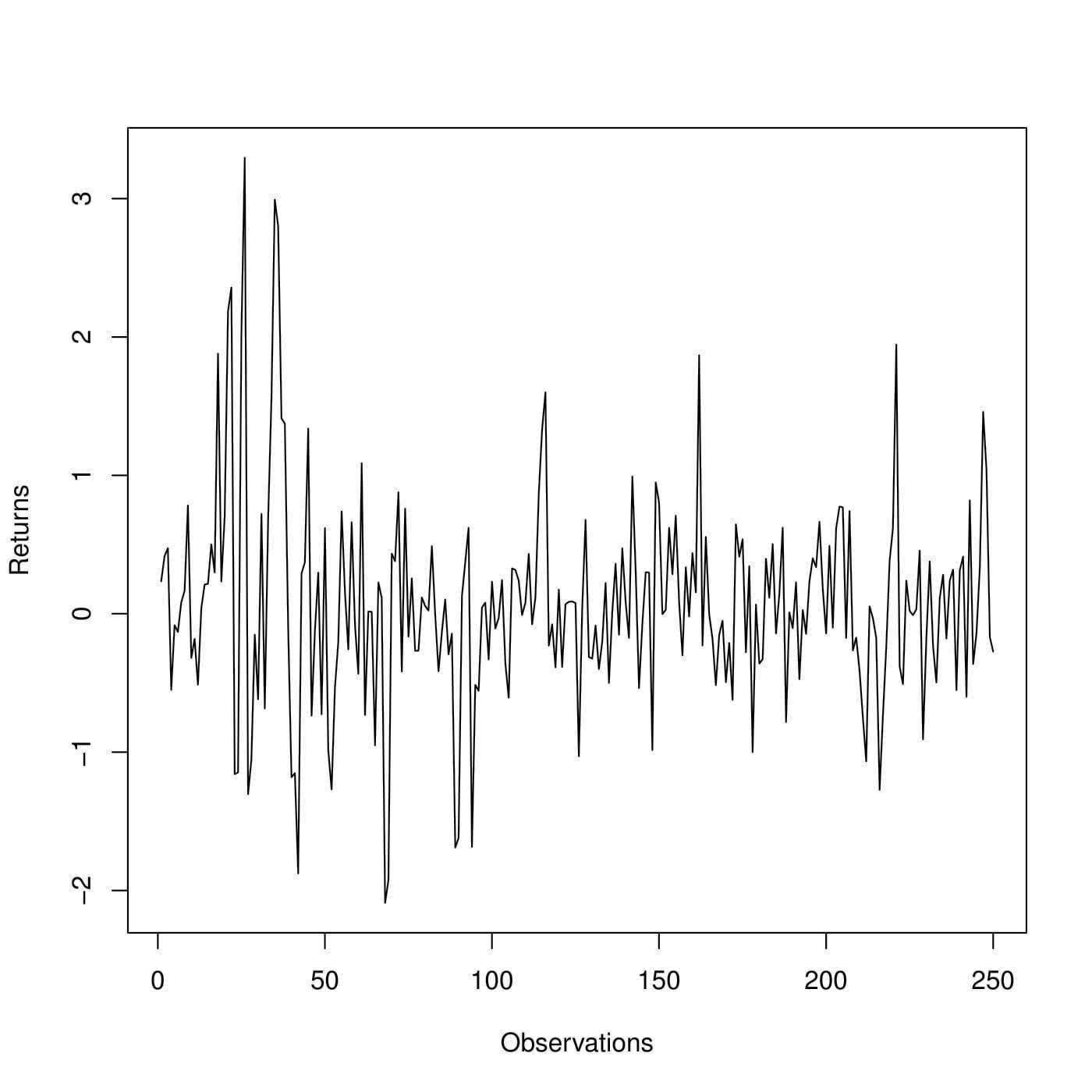
In the following, we illustrate the above approach with the use of a numerical example. Our dataset consists of daily returns from the MASI index covering the period of 15th November 2016 to the 15th November 2017, which includes a total of observations. The MASI (Moroccan All Shares Index) is a stock index that tracks the performance of all securities listed in the Casablanca Stock Exchange located at Casablanca in Morocco.444http://www.casablanca-bourse.com
The proposed methodology does not make any assumptions about the distribution that describes the data, except that an Augmented Unit Root test is performed to make sure that our data series is stationary. Moreover, as shown in Figure 1, the return graph validates this verification since the series fluctuates around 0 and has no trend.
Remark 5.2.
When defining the we were making the convention that our rv represents financial losses (profits) when it has positive (negative) values. However, to be in compliance with the real world data the latter convention is updated.
By using the sorted returns series we calculate the value to identify the concerned losses. Then, we affect to each value its own weight in accordance with the parameters and as shown below in Table 1.
To fulfill the condition we take arbitrarily as the midpoint of the interval, thus .
| Sorted Returns(%) | Weights |
|---|---|
| ⋮ | ⋮ |
| -1.146 | 0.04 |
| -1.151 | 0.05 |
| -1.160 | 0.05 |
| -1.181 | 0.06 |
| -1.270 | 0.06 |
| -1.273 | 0.07 |
| -1.304 | 0.08 |
| -1.621 | 0.08 |
| -1.685 | 0.09 |
| -1.690 | 0.10 |
| -1.880 | 0.10 |
| -1.924 | 0.11 |
| -2.090 | 0.11 |
In Table 2 below, we report the calculation results of for different values of and :
| 1.32% | 1.28% | 1.25% | 1.22% | 1.22% | |
| 1.58% | 1.55% | 1.52% | 1.50% | 1.49% | |
| 1.99% | 1.98% | 1.97% | 1.96% | 1.96% | |
This empirical exercise using the daily returns for the MASI index between 15th November 2016 and 15th November 2017 is a historical approach that illustrates the practical use of in the real world by considering the psychological attitude of the investor. The obtained results confirm earlier remarks in the previous subsection: first, more the investor is risk averse less risks he takes and then smaller is the amount of capital required to hedge his position; furthermore, we have and in a highly risk averse context ( for this survey) both risk measures can be confounded.
References
- [1] Acerbi, C. (2002). Spectral measures of risk: A coherent representation of subjective risk aversion. Journal of Banking and Finance, 26, 1505-1518. doi: 10.1016/S0378-4266(02)00281-9
- [2] Artzner, P., Delbaen, F., Eber, J.-M. and Heath, D. (1999). Coherent measures of risk. Mathematical Finance, 9, 203-228. doi: 10.1111/1467-9965.00068
- [3] Ceriani, L. and Verme, P. (2012). The origins of the Gini index: extracts from Variabilità e Mutabilità (1912) by Corrado Gini. Journal of Economic Inequality, 10, 421-443. doi: 10.1007/s10888-011-9188-x
- [4] Choquet, G. (1954). Theory of capacities. Annales de l’institut Fourier, 5, 131-295. doi: 10.5802/aif.53
- [5] Dana, R.-A. (2005). A representation result for concave Schur-concave functions. Mathematical Finance, 15, 613-634. doi: 10.1111/j.1467-9965.2005.00253.x
- [6] Delbaen, F. (2012): Monetary Utility Functions. Osaka University Press, Osaka.
- [7] Embrechts, P., Puccetti, G., Rüschendorf, L., Wang, R. and Beleraj, A. (2014). An academic response to Basel 3.5. Risks, 2, 25-48. doi:10.3390/risks2010025
- [8] Fischer, T. (2003). Risk capital allocation by coherent risk measures based on one-sided moments. Insurance: Mathematics and Economics 32, 135-146. doi: 10.1016/S0167-6687(02)00209-3
- [9] Föllmer, H. and Schied, A. (2011). Stochastic Finance: An Introduction in Discrete Time. (Third Edition.) Walter de Gruyter, Berlin.
- [10] Furman, E. and Landsman, Z. (2006). Tail variance premium with applications for elliptical portfolio of risks. ASTIN Bulletin: Journal of the International Actuarial Association, 36, 433-462. doi: 10.2143/AST.36.2.2017929
- [11] Furman, E., Wang, R. and Zitikis, R. (2017). Gini-type measures of risk and variability: Gini shortfall, capital allocation and heavy-tailed risks. Journal of Banking and Finance. In Press, Accepted Manuscript. doi: 10.1016/j.jbankfin.2017.06.013
- [12] Giorgi, G.M. (1990) Bibliographic portrait of the Gini concentration ratio. Metron, 48, 183-221.
- [13] Giorgi, G.M. (1993) A fresh look at the topical interest of the Gini concentration ratio. Metron, 51, 83-98.
- [14] Grechuk, B., Molyboha, A. and Zabarankin, M. (2009). Maximum entropy principle with general deviation measures. Mathematics of Operations Research, 34, 445-467. doi: 10.1287/moor.1090.0377
- [15] Mao, T. and Wang, R. (2016). Risk aversion in regulatory capital principles. Working paper. doi: 10.2139/ssrn.2658669
- [16] McNeil, A.J., Frey, R. and Embrechts, P. (2005). Quantitative Risk Management: Concepts, Techniques and Tools. (Revised Edition.) Princeton University Press, Princeton, NJ.
- [17] Righi, M. and Ceretta, P. (2016). Shortfall Deviation Risk: an alternative to risk measurement. Journal of Risk 19, 81-116. doi: 10.21314/JOR.2016.349
- [18] Righi, M. and Borenstein, D. (2017). A simulation comparison of risk measures for portfolio optimization. Finance Research Letters, in press. doi: 10.1016/j.frl.2017.07.013
- [19] Righi, M. (2017). A composition between risk and deviation measures. Working Paper.
- [20] Rockafellar, R. T., Uryasev, S. and Zabarankin, M. (2006). Generalized deviation in risk analysis. Finance and Stochastics, 10, 51-74. doi: 10.1007/s00780-005-0165-8
- [21] Rüschendorf, L. (2013). Mathematical Risk Analysis. Dependence, Risk Bounds, Optimal Allocations and Portfolios. Springer, Heidelberg.
- [22] Schmeidler, D. (1986). Integral representation without additivity. Proceedings of the American Mathematical Society, 97, 255-261. doi: 10.2307/2046508
- [23] Schmeidler, D. (1989). Subject probability and expected utility without additivity. Econometrica, 57(3), 571-587. doi: 10.2307/1911053
- [24] Shalit, H., and Yitzhaki, S. (1984). Mean-Gini, portfolio theory and the pricing of risky assets. Journal of Finance, 39(5 (December)), 1449-1468. doi: 10.1111/j.1540-6261.1984.tb04917.x
- [25] Wang, R., Wei, Y. and Willmot., G.E. (2017). Characterization, Robustness and Aggregation of Signed Choquet Integrals. Working paper.
- [26] Yaari, M.E. (1987). The dual theory of choice under risk. Econometrica, 55, 95-115. doi: 10.2307/1911158
- [27] Yitzhaki, S. (1983) On an extension of Gini inequality index. International Economic Review, 24, no. 3, 617-628. doi: 10.2307/2648789
- [28] Yitzhaki, S. (1998) More than a dozen alternative ways of spelling Gini. Research on Economic Inequality, 8, 13-30. doi: 10.1007/978-1-4614-4720-7
- [29] Yitzhaki, S. and Schechtman, E. (2005). The properties of the extended Gini measures of variability and inequality. Metron, LXIII(3), 401-443. doi: 10.2139/ssrn.815564
- [30] Yitzhaki, S. and Schechtman, E. (2013). The Gini Methodology: A Primer on a Statistical Methodology. Springer, New York, NY.