Extending the centerpoint theorem to multiple points
Abstract
The centerpoint theorem is a well-known and widely used result in discrete geometry. It states that for any point set of points in , there is a point , not necessarily from , such that each halfspace containing contains at least points of . Such a point is called a centerpoint, and it can be viewed as a generalization of a median to higher dimensions. In other words, a centerpoint can be interpreted as a good representative for the point set . But what if we allow more than one representative? For example in one-dimensional data sets, often certain quantiles are chosen as representatives instead of the median.
We present a possible extension of the concept of quantiles to higher dimensions. The idea is to find a set of (few) points such that every halfspace that contains one point of contains a large fraction of the points of and every halfspace that contains more of contains an even larger fraction of . This setting is comparable to the well-studied concepts of weak -nets and weak -approximations, where it is stronger than the former but weaker than the latter. We show that for any point set of size in and for any positive where and for every with we have that , we can find of size such that each halfspace containing points of contains least points of . For two-dimensional point sets we further show that for every and with and we can find with such that each halfplane containing one point of contains at least of the points of and each halfplane containing all of contains at least points of . All these results generalize to the setting where is any mass distribution. For the case where is a point set in and , we provide algorithms to find such points in time .
1 Introduction
Medians and quantiles are ubiquitous in the statistical analysis and visualization of data. These notions allow for quantifying how deep some point lies within a one-dimensional data set by measuring how many elements of the data set appear before the point and how many appear after it. In comparison to the mean, medians and quantiles have the advantage that they only depend on the order of the data points, and not their exact positions, making them robust against outliers. However, in many applications, data sets are multidimensional, and there is no clear order of the data set. For this reason, various generalizations of medians to higher dimensions have been introduced and studied. Many of these generalized medians rely on a notion of depth of a query point within a data set, a median then being a query point with the highest depth among all possible query points. Several such depth measures have been introduced over time, most famously Tukey depth [19] (also called halfspace depth), simplicial depth, or convex hull peeling depth (see, e.g., [1]). All of these depth measures lead to generalized medians that are invariant under affine transformations. As for quantiles, only a few generalizations have been introduced (see, e.g., [7]). We propose such a generalization by extending a depth measure to sets with a fixed number of query points and defining a quantile as a set with maximal depth. The depth measure we extend is Tukey depth: the Tukey depth of a point with respect to a point set is the minimal number of points of in any closed halfspace containing . More formally, if denotes the set of closed halfspaces, then the Tukey depth of with respect to is
Similarly, the Tukey depth can also be defined for a mass distribution :
Here, a mass distribution on is a measure on such that all open subsets of are measurable, and for every lower-dimensional subset of .
The centerpoint theorem states that there is always a point of high depth, i.e., a point such that for every closed halfspace containing we have (or for masses). Note that, for , such a centerpoint is a median: a median has the property that every halfline containing it contains at least half of the underlying data set. Quantiles can be interpreted similarly: the -quantile and the -quantile form a set of two points such that every halfline that contains one of them contains at least of the data set. Furthermore, a halfline containing both of the points contains at least of the underlying data set. In particular, halflines containing more points contain more of the data set. This idea leads to the following generalization of Tukey depth for a set of multiple points:
Again, we can generalize this to mass distributions:
We prove that there is always a set of points that has generalized Tukey depth . In fact, we prove the following, more general statement:
Theorem 1.
Let be a mass distribution in with . Let be non-negative real numbers such that and for every with we have that . Then there are points in such that for each closed halfspace containing of the points we have .
Note that, for and , the points and correspond to the -quantile and the -quantile; for we get our bound on the generalized Tukey depth, and for , the result implies the centerpoint theorem.
Our second result is motivated by interpreting the -quantile and the -quantile not as two points, but as a one-dimensional simplex. We then have that every halfline that contains a part of the simplex contains at least of the underlying data set and every halfline that contains the whole simplex contains at least of the underlying data set. Also for this interpretation we give a generalization to two dimensions:
Theorem 2.
Let be a mass distribution in with . Let and be real numbers such that and . Then there is a triangle in such that
-
(1)
for each closed halfplane containing one of the vertices of we have and
-
(2)
for each closed halfplane fully containing we have .
Note that this again generalizes centerpoints for . However, this result does not give bounds on the generalized Tukey depth of these sets, as, e.g., a halfspace containing two points may still only contain an -fraction of the mass.
Finally, we give algorithms to compute two points satisfying the two-dimensional case of Theorem 1 and three points satisfying Theorem 2 in time .
Related work
Another way to view our setting is the following: given a multidimensional data set, we want to find a fixed number of representatives. The idea of small point sets representing a larger point set has been studied in many different settings. One of the most famous of those is the concept of -nets, introduced by Haussler and Welzl [8]. For a range space , consisting of a set and a set of subsets of , an -net on is a subset of with the property that every with intersects . In our setting, where we consider halfspaces, we would choose and as the set of all halfspaces. It is known that for this range space, for any point set there exists an -net of size . In particular, this bound does not depend on the size of . Note that we require the -net to be a subset of . If this condition is dropped, we arrive at the concept of weak -nets. The fact that the points for the weak -net can be chosen anywhere in allows for very small weak -nets for many range spaces. There has been some work on weak -nets of small size. For halfplanes in for example, Aronov et al. [4] have shown that there is always a weak -net of two points. These two points both lie outside of the convex hull of . They also consider many other range spaces, such as convex sets, disks and rectangles. Similarly, Babazadeh and Zarrabi-Zadeh [5] construct weak -nets of size 3 for halfspaces in . For two-dimensional convex sets, Mustafa and Ray [16] have shown that there is always a weak -net of two points; Shabbir [18] shows how to find two such points in time.
Another related concept is the concept of -approximations: For a range space an -approximation on is a subset of with the property that for every we have . Again, the restriction that has to be a subset of can be dropped to get the notion of weak -approximations. Just as for -nets, there has been a lot of work on -approximations and weak -approximations, see [15] for a recent survey. In particular it was shown that for halfspaces in , there always is an -approximation of size [13, 14].
While our setting can be considered to be related to weak -nets and weak -approximations for range spaces determined by halfspaces, the differences are significant. As we will discuss here, a halfspace missing all the points of may still contain up to half of the points of the initial set, and thus qualifies neither as a good weak -approximation nor -net.
Note that for , the condition of Theorem 1 that any halfspace containing all of the points of contains at least points of is equivalent to the statement that every halfspace containing more than of the points of contains at least one point of . So, is a weak -net of . Furthermore, the condition that any halfspace containing one of the points of contains at least points of translates to the statement that every halfspace containing more than of the points of must contain all of . Thus, is not only a weak -net of but also has the additional property that all points of are somewhat deep within . (For two points in the plane, this comes at the cost of having larger than .) On the other hand, while we require halfspaces containing all points of to also contain many points of , we also allow halfspaces containing only one point of to contain many points of . This separates our concept from weak -approximations. Note that when dealing with halfspaces and -nets of size 2, the weak -net of Aronov et al. [4] is actually also a weak -approximation. Similarly, Theorem 1 gives us a weak -approximation of , with the optimal value being reached when tends to zero (which actually corresponds to the result in [4]). Adding more points to does not give us a better approximation. For , requiring that for we have implies , so a halfspace containing no points of may contain half of the points of ; we therefore cannot get anything better than a weak -approximation. Also, we do not get anything better than a weak -net.
In fact, our setting is very much related to the concept of one-sided -approximants, recently introduced by Bukh and Nivasch [6]: For a range space , a one-sided -approximant on is a subset of with the property that for every we have . Once again, the restriction that has to be a subset of can be dropped to get the notion of weak one-sided -approximations. Note that the only difference to the definition of -approximations is that one does not take the absolute value of the difference. In particular, if , i.e., if contains many points of despite containing only few points of , the difference is negative, and thus smaller than .
In their paper, Bukh and Nivasch [6] consider the range space of convex sets. They show that any point set in allows a one-sided -approximant for convex ranges of size , where only depends on and , but not on the size of .
In a similar reasoning, it makes sense to define an approximation by a set such that for every we have . Intuitively, if a range contains a large fraction of the points of , then it is guaranteed to contain a large fraction of the set we want to approximate. But here again, our approximation ratio is at best.
2 Two points
We first consider the case where the underlying data is a point set. Motivated by the definition of generalized Tukey depth, we consider and . Even though this result is a special case of Theorem 1, we still show its proof for two reasons: first, the Algorithm presented in Section 5 relies heavily on the presented proof and, secondly, the proof already illustrates the main ideas for the proof of Theorem 1.
Theorem 3.
Let be a set of points in general position in the plane. Then there are two points and in such that
-
(1)
each closed halfplane containing one of the points and contains at least of the points of and
-
(2)
each closed halfplane containing both and contains at least of the points of .
Proof.
Note that condition (1) is equivalent to the condition that every open halfplane containing more than of the points of must contain both and . Similarly, condition (2) is equivalent to the condition that every open halfplane containing more than of the points of must contain one of and . We will now construct two points and satisfying both these conditions.
Let be the intersection of all open halfplanes containing more than of the points of . Clearly is convex. Also, note that is closed. The centerpoint region is a strict subset of and thus has a non-empty interior. In order to satisfy condition (1), both and have to be placed in .
Let now be the set of all open halfplanes containing more than of the points of . For any in let be the intersection of and . In order to also satisfy condition (2), we need to find two points and such that every contains at least one of them. To this end, we partition into two subsets and . The set contains all halfplanes that lie on the left side of their respective boundary lines. Analogously, contains all halfplanes that lie on the right side of their respective boundary lines. For a halfplane that has a horizontal boundary line, we put in if and only if it lies above its boundary line.
Note that any three halfplanes in have a non-empty intersection: Consider the inclusion-minimal halfplane with horizontal boundary line and its intersection with the boundary of the convex hull of . As is open, is not in . However, we claim that any point in on the convex hull boundary of in an -neighborhood of is in any halfplane of . Indeed, if there was a halfplane in not containing , it would contain a strict subset of the intersection of the convex hull of with ; however, this would contradict the minimality of . The analogous holds for .
We will now show that for any two halfplanes and in , their corresponding regions and have a non-empty intersection. The same arguments hold for any two halfplanes in . Assume for the sake of contradiction that and do not intersect. As and are convex, this means that there is an open halfplane containing more than of the points of such that the intersection of the boundary lines of and lies in , the complement of (see Figure 1). In particular, is a strict subset of . As contains strictly fewer than of the points of and contains strictly fewer than of the points of , must contain strictly more than of the points of . However, being a subset of , which also contains strictly fewer than of the points of , this is a contradiction. Thus, by contradiction, and intersect.

As neither three halfplanes in nor two halfplanes in and have an empty intersection, Helly’s Theorem entails that there exists a point in both and all halfplanes in , i.e., all s associated to have a non-empty intersection . Again, the same holds for , with a non-empty intersection . Placing in and in , we have thus constructed two points such that the conditions (1) and (2) hold. ∎
This result is tight in the following sense: There is a point set for which it is not possible to improve both conditions at the same time, that is, it is not possible to find two points such that any halfplane containing one of them contains strictly more than of the points and any halfplane containing both of them contains strictly more than of the points. For this consider a set of point arranged in the following way. Partition the points into 5 sets of points each. Place in such a way that the convex hull of each is disjoint from the convex hull of the union of the other four sets (see Figure 2).

Denote by the convex hull of . Let be a line through and . Note that any other set is not separated by (i.e., lies entirely on one side). Let be the side of containing fewer of the other sets and let be the other side. For any point in we say that is above if it is not in but it is in . Similarly, for any point in we say that is below if it is not in but it is in . Suppose, for the sake of contradiction, that there exist two points and such that any halfplane containing one of them contains strictly more than of the points of and any halfplane containing both of them contains strictly more than of the points of . Consider two sets and such that contains exactly one other set. First we note that neither nor can lie above as otherwise we can find a halfplane containing that point and only one of the sets, i.e., only points. Similarly, we cannot place both and below , as otherwise we can find a halfplane containing both points and only two of the sets, i.e., only points. Also, we must clearly place both and in . Thus, for any two sets and such that contains exactly one other set, must contain at least one of and . However, there are five such and can be placed in such a way that no three of them have a common intersection. So no matter how we place and , one of the will be empty.
3 An arbitrary number of points
We now strengthen Theorem 3 in four ways: we allow for arbitrarily many query points, we extend it to higher dimensions, we consider mass distributions instead of point sets, and we give a range of possible bounds:
See 1
We use the following observation, which follows from the fact that for an empty intersection of halfspaces, any point with non-zero mass is in at most such halfspaces.
Observation 4.
Let be a mass distribution in with . Let be open halfspaces with . Then .
Proof of Theorem 1.
The result is straightforward for , so assume . Again the condition that for each closed halfspace containing of the points we have is equivalent to the condition that every open halfspace with must contain at least of the points . Let . For , we call an open halfspace a -halfspace if . Consider the --plane, denoted by , and for each vector in let be the projection of to . Let be unit vectors in with the property that the angle between any and is . Note that this implies that also the angle between and is . For each we construct a principal set of halfspaces as follows: For each , consider all -halfspaces. For any such halfspace , let be the normal vector to its bounding hyperplane that points into . Let be in if the angle between and is at most . If , place arbitrarily in of the ’s. Note that with this construction each -halfspace is contained in exactly principal sets. Thus, if, for each principal set, we can pick a point in all its halfplanes, then each -halfplane contains points.
It remains to show that the halfspaces in each principal set have a common intersection. Let be halfspaces in and assume for the sake of contradiction that they have no common intersection. Then the positive hull (conical hull) of their projected normal vectors must be , and in particular there are three of them, w.l.o.g. , and , whose projected normal vectors already have as their positive hull. Further, among those three halfspaces, there are two of them, w.l.o.g. and , such that the angles between their projected normal vectors and sum up to more than . If is a -halfspace, then by construction of we have that the angle between and is at most . Analogously, if is a -halfspace, the angle between and is at most . By the choice of and we thus have , which is equivalent to , and to , as and are integers. By definition of a -halfspace we have
Furthermore we have for every , and thus
which is equivalent to
As , we have that and thus , which is a contradiction to Observation 4. ∎
Setting , we get a bound for the generalized Tukey depth:
Corollary 5.
Let be a mass distribution in with . Then there exist points in with generalized Tukey depth .
4 Triangles
As mentioned before, the -quantile and the -quantile can also be interpreted as a one-dimensional simplex with the property that every halfline that contains a part of the simplex contains at least of the underlying data set and every halfline that contains the whole simplex contains at least of the underlying data set. For this interpretation, we give a generalization to two dimensions. For ease of presentation, we only give a proof for point sets instead of mass distributions and for fixed values of and .
Theorem 6.
Let be a set of points in general position in the plane. Then there are three points , and in such that
-
(1)
each closed halfplane containing one of the points , and contains at least of the points of and
-
(2)
each closed halfplane containing all of , and contains at least points of .
Note that this can also be interpreted as an instance of Theorem 1 with and . However, as , the precondition of Theorem 1 does not apply. The proof of this result uses similar ideas as the above proofs.
Proof of Theorem 6.
Let be the intersection of all open halfplanes containing more than of the points of . Just as in the proof of Theorem 3, condition (1) is equivalent to , and lying in . Similarly, condition (2) is equivalent to the following statement: for every open halfplane containing more than of the points of , contains at least one of , and . For the latter, let be a vector and let be the set of all of these halfplanes that have as their normal vector. The intersection of all elements of is a closed halfspace . Let be the set of all of these , i.e., for every possible direction of . Then, condition (2) is equivalent to the following statement: for every halfplane in , contains at least one of , and . For each such halfplane , let be the intersection of and . Note that is compact. We thus want to show the claim that we can find three points , and such that each contains at least one of them. Let be the set of s that are minimal with respect to set inclusion. Clearly, it is enough to show the claim just for the elements of . Let be the set of normal vectors of the defining halfplanes of the elements of . Note that there is a natural mapping from to a subset of the unit circle . We will say that a subset of is connected, if its image under this mapping to is connected.
First we show that among any three elements of , two of them intersect. Let , and be elements of , and let , and be their associated halfplanes. Assume for the sake of contradiction that , and are pairwise disjoint. Let be the normal vector of . Let be the positive hull of , and . Then is either a cone or the whole plane. See Figure 3. If is the whole plane, then , and have no common intersection. Otherwise, if is a cone, then one of , and can be described as a positive linear combination of the other two. In particular, , and have a common intersection and one of them is redundant in the description of . We thus consider two cases, namely whether , and have a common intersection or not.

First, assume that , and have no common intersection. Then , and partition the plane into seven regions (see Figure 4): for , , for all different and . Note that each contains strictly fewer than of the points of , as otherwise the corresponding and intersect. In particular, contains more than points of . It follows that and thus also contains strictly fewer than of the points of . The number of points in is the sum of the number of points in , and . All of these sets contain strictly fewer than of the points of , implying that contains fewer than of the points of , which is a contradiction. This concludes the first case.

For the second case assume that , and have a common intersection and one of the halfplanes is redundant in the description of ; assume without loss of generality that it is . Just as in the first case, each contains strictly fewer than of the points of . Again it follows that contains strictly fewer than of the points of . The sets , and cover , implying that contains fewer than of the points of , which is again a contradiction. This concludes the proof that among any three elements of , two intersect.
It remains to show that we can find three points , and such that each element of contains at least one of them. This can be achieved by picking one element of and placing two points and at the extreme intersection points with the boundary of ; since any three elements of intersect, any two elements not containing and must intersect and we may apply Helly’s theorem in dimension one. However, we actually have more flexibility in choosing .Note that the normal vectors pointing into the halfplanes defining the elements of define a circular order on . Place at a topmost point of the boundary of . Let be the first element of in counterclockwise direction whose defining halfplane does not contain in its interior. Place at the intersection of the defining line of with the boundary of that is furthest in counterclockwise direction from . Since is minimal, any element of intersecting contains either or . (Note that so far does not contain any of or .) Therefore, all elements of that do not intersect have a common intersection, in which we place . Recall that the defining halfplanes are open and therefore there is no element of intersecting in a single point. We therefore may move slightly in clockwise direction, such that it is also contained in . ∎
The general statement can be proved analogously: See 2
5 Construction in the plane
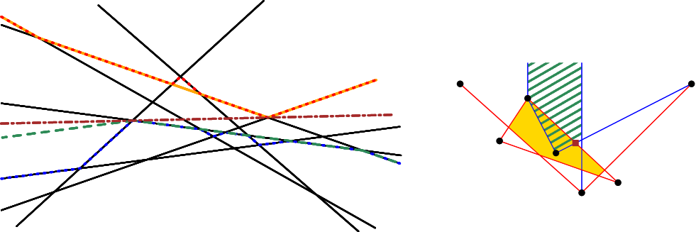
In this section, we describe algorithms for constructing the points described in Theorems 3 and 6. We first observe that the convex regions defined by the intersections of the half-planes in sets like and in the proof of Theorem 3 correspond to levels in the dual line arrangement. We use the duality that maps a point to a line . The -level of a line arrangement is the set of points with exactly lines below it and not more than lines above it. (It thus consists of segments of the line arrangement.) Suppose we are given and , s.t. and . Let be the set of open halfplanes that are above their boundary lines and contain more than points of , and let be their intersection. A point is in if there is no line through it having at least points of above it. If the dual line of contains a point below the -level of the dual line arrangement of , then has a supporting line with more than points of above it. Since a line has a point below that level if and only if it intersects the interior of its convex hull, the interior of the convex hull of the -level thus excludes exactly those lines whose primal points are not in . The supporting lines of the segments of the convex hull of the -level give the primal points that bound . Matoušek [11] describes an algorithm for constructing the -level of a line arrangement in time. The -hull of a set of points in the plane is the set of points in such that any closed halfplane defined by a line through contains at least points of . The set in the proof of Theorem 3 is the intersection of all open halfplanes containing more than points. is thus the -hull of . The -hull of is obtained by computing the convex hulls of the -level and the -level of the dual line arrangement of , which give the upper and lower envelope of the -hull [11]. To construct the points from Theorems 3 and 6 (without explicitly constructing the levels), we use Matoušek’s algorithmic tools from [11].
Lemma 7 (Matoušek [11, Lemma 3.2]).
In an arrangement of lines, let be the boundary of the convex hull of the lines on or below the -level. Given the arrangement, , and a point , one can find the tangent to passing through and touching to the right of (if it exists) in time .
Lemma 8.
Given an arrangement of lines and two numbers , as well as a halfplane , a line separating the -level from the intersection of with the -level can be found in time, if it exists. The separating line is tangent to both level parts and, from left to right, first intersects the -level and then the relevant part of the -level.
Proof.
Let be the boundary of the convex hull of all points below the -level, and let be the intersection of with the -level. Note that might not be connected. Suppose we want our line to be the counterclockwise bitangent of and (i.e., from left to right, it first intersects , which has no point above it, and then ). Our algorithm works by obtaining tangents to through points on . Matoušek’s algorithm for determining the tangent to a level through a given point that is to the right of that point [11, Lemma 3.2] (our Lemma 7) also directly works for parts of a level such as : It requires a sub-algorithm that decides in time whether a given line intersects the level (or, in our case, the partial level ). This can be done by sorting the intersection of the lines of the arrangements along (see also [11, Lemma 3.1]) as well as along the line bounding ; either intersects the relevant part of , or we can compare the intersection of with to the intersections of with to determine whether there is a point of below .
Suppose first we are given . (It requires time though to obtain it, so we eventually get rid of this assumption.) The convex hull of a level is known to have at most vertices [11, Lemma 2.1]. For a point on , we can find in time the point on such that the line has no point on below it. We can thus find, by binary search on the vertices of , a vertex with on such that separates and . This gives an time algorithm for obtaining the bitangent. To improve on that bound, we need to get rid of the explicit construction of to find the tangents to .
To this end, we consider Matoušek’s algorithm for constructing the convex hull boundary of a level and compute only the relevant part (see [11, Section 4]). In particular, the algorithm works by finding, for a constant and two vertical lines, further vertical lines between the given ones such that there are at most crossings of the arrangement between two of these verticals. This can be done in time (as described in [12]). The tangents on at the intersection points with the vertical lines can be computed in time [11, Lemma 3.3]. It is shown in [11] that, when choosing , there are at most lines of the arrangement relevant for the construction of between two such vertical lines, and these lines can be found in time. The original algorithm proceeds recursively within each interval defined by two neighboring vertical lines after removing the non-relevant lines. In our adaption, however, we find the interval that contains the point on such that a tangent to through the vertex with on such that separates and . (We do this by considering the tangent to at each of the constant number of intersection of a vertical line with .) When we have found this interval, we can prune of the lines and recurse inside this interval. Note, however, that we cannot prune the set of lines when looking for a tangent to . Thus, in each recursive call, we need time for computing the tangent. As the recursion depth is , this amounts to in total. Also, for lines during the th recursion, we need time for determining the intervals. As decreases geometrically, this also amounts to . This is the total running time for finding the bitangent, as claimed. ∎
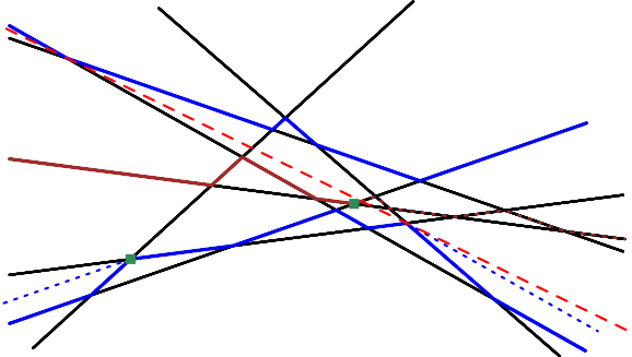
We call such a line the counterclockwise bitangent of the two subsets of the plane (i.e., the intersection with the region not above it has smaller -coordinate than the intersection with the region not below it). Note that by mirroring the plane horizontally or vertically, the lemma also provides other types of bitangents. Figure 5 shows an example.
Lemma 8 can also be obtained using the framework of Langerman and Steiger [10], similar to the computation of the Oja depth in [3]. (We merely sketch its application in this paragraph.) Let be the primal point set of the arrangement. In the formulation of [3], if there exists a function that has the minimum on the intersection of supporting lines of point pairs of with the property that, for a given point , we can find in time a witness halfplane through such that for all points in that halfplane, we have , then there is an time algorithm for finding such a minimum point. We can test in time whether the dual of intersects or , defining a witness halfplane using the primal of such an intersection point (as described at the beginning of the previous proof), or the intersection point of with the line defining . If the dual line separates from , we need a separator with a larger slope to obtain a counterclockwise bitangent, and thus define a witness halfplane to the right of a vertical line through .
Lemma 8 can now be used to obtain the following result.
Theorem 9.
Given a set of points in the plane, two points satisfying the conditions of Theorem 3 can be constructed in time .
Proof.
To find a point in the intersection of and , observe first that we can restrict our attention in the dual to the convex hull of the points above the -level of the dual line arrangement. This is because any primal line with more than points above it (which corresponds to a dual point below the -level) also defines a halfplane in . A point in the intersection of and thus corresponds to a line on or above the -level and on or below the -level. We find a bitangent to these two levels in time using Lemma 8 (with ). The primal point of this line is ; see the point indicated by the brown box in Figure 5 (right). We obtain analogously. ∎
Theorem 10.
Three points as described in Theorem 6 can be computed in time .
Proof.
Consider the dual line arrangement of the point set. The points dualize to three lines that are between the -level and the -level of the arrangement s.t. every point on the middle level has at least one of these lines above it and one of these lines below it. (We assume for simplicity that is odd and the middle level is the -level of the arrangement; if is even, one has to consider the points between the -level and the -level.) Theorem 6 asserts that such lines exist, and its proof tells us that we can choose one of these lines to be an arbitrary tangent of one of the levels not intersecting the interior of the other one. We denote by and the convex hull boundaries of the points on or below the -level and of the points on or above the -level, respectively.
We let be the clockwise bitangent of and , which we can obtain in time using Lemma 8. For simplicity of explanation, we also compute the counterclockwise bitangent . (This step may be omitted in an actual implementation, but assuming it to be given facilitates the explanation and does not change the asymptotic running time.)
The line intersects the middle level of the arrangement. Let be the parts of the middle level below , and be the part above it. Note that each of these parts may be disconnected. Using Lemma 8, we search for the counterclockwise bitangent between (or, equivalently, the -level) and (which is the intersection of the middle level with a halfspace defined by ) in time. If it exists, and its intersection point with is between the intersections of with and , we choose this line to be . Otherwise, we continue our search on in the same way (i.e., we look for the counterclockwise bitangent between and ). The line can be found in an analogous manner. ∎
6 Conclusion
We proposed a generalization of quantiles in higher dimensions based on a generalization of Tukey depth to multiple points. Our bounds and algorithms seem merely being a first step in this direction and we can identify several interesting open problems. Except for special cases of Theorem 1, we do not believe that our bounds are tight and particularly expect significantly better bounds in higher dimensions. Naturally, there are many other range spaces for which this problem could be considered, e.g., convex sets, like in [6].
From an algorithmic point of view, the bottleneck for the running time of our approach is Lemma 8. The current methods result in time. While solutions to such kinds of problems can usually only be verified in time (see, e.g., [2, 17]), a linear-time algorithm, like for centerpoints [9], is conceivable. For arbitrarily many points, it seems tedious but doable to apply similar approaches as in the proof of Theorem 9. Is there a good bound on the running time independent of the size of ?
Acknowledgments.
We thank Emo Welzl for initiating discussions on this topic, as well as anonymous reviewers for helpful comments.
References
- [1] Greg Aloupis. Geometric measures of data depth. In Regina Y. Liu, Robert Serfling, and Diane L. Souvaine, editors, Data Depth: Robust Multivariate Analysis, Computational Geometry and Applications, pages 147–158. DIMACS/AMS, 2003.
- [2] Greg Aloupis, Carmen Cortés, Francisco Gómez, Michael Soss, and Godfried Toussaint. Lower bounds for computing statistical depth. Comput. Statist. Data Anal., 40(2):223–229, 2002. doi:10.1016/S0167-9473(02)00032-4.
- [3] Greg Aloupis, Stefan Langerman, Michael A. Soss, and Godfried T. Toussaint. Algorithms for bivariate medians and a Fermat-Torricelli problem for lines. Comput. Geom., 26(1):69–79, 2003. doi:10.1016/S0925-7721(02)00173-6.
- [4] Boris Aronov, Franz Aurenhammer, Ferran Hurtado, Stefan Langerman, David Rappaport, Carlos Seara, and Shakhar Smorodinsky. Small weak epsilon-nets. Comput. Geom., 42(5):455–462, 2009. doi:10.1016/j.comgeo.2008.02.005.
- [5] Maryam Babazadeh and Hamid Zarrabi-Zadeh. Small weak epsilon-nets in three dimensions. In Proc. 18th Canadian Conference on Computational Geometry (CCCG), 2006.
- [6] Boris Bukh and Gabriel Nivasch. One-sided epsilon-approximants. In Martin Loebl, Jaroslav Nešetřil, and Robin Thomas, editors, A Journey Through Discrete Mathematics: A Tribute to Jiří Matoušek, pages 343–356. Springer, 2017. doi:10.1007/978-3-319-44479-6_12.
- [7] Probal Chaudhuri. On a geometric notion of quantiles for multivariate data. J. American Statist. Assoc., 91(434):862–872, 1996.
- [8] David Haussler and Emo Welzl. -nets and simplex range queries. Discrete Comput. Geom., 2:127–151, 1987. doi:10.1007/BF02187876.
- [9] Shreesh Jadhav and Asish Mukhopadhyay. Computing a centerpoint of a finite planar set of points in linear time. Discrete Comput. Geom., 12:291–312, 1994. doi:10.1007/BF02574382.
- [10] Stefan Langerman and William L. Steiger. Optimization in arrangements. In 20th Symp. on Theoretical Aspects of Computer Science (STACS), volume 2607 of LNCS, pages 50–61, 2003. doi:10.1007/3-540-36494-3_6.
- [11] Jiří Matoušek. Computing the center of planar point sets. In Jacob E. Goodman, Richard Pollack, and William Steiger, editors, Discrete and Computational Geometry: Papers from the DIMACS Special Year, volume 6 of DIMACS Series in Discrete Mathematics and Theoretical Computer Science, pages 221–230. DIMACS/AMS, 1990.
- [12] Jiří Matoušek. Construction of epsilon-nets. Discrete Comput. Geom., 5:427–448, 1990. doi:10.1007/BF02187804.
- [13] Jiří Matoušek. Tight upper bounds for the discrepancy of half-spaces. Discrete Comput. Geom., 13(3):593–601, 1995. doi:10.1007/BF02574066.
- [14] Jiří Matoušek, Emo Welzl, and Lorenz Wernisch. Discrepancy and approximations for bounded VC-dimension. Combinatorica, 13(4):455–466, 1993. doi:10.1007/BF01303517.
- [15] Nabil Mustafa and Kasturi Varadarajan. Epsilon-approximations and epsilon-nets. In Handbook of Discrete and Computational Geometry. 2017.
- [16] Nabil H. Mustafa and Saurabh Ray. An optimal extension of the centerpoint theorem. Comput. Geom., 42(6):505–510, 2009. doi:10.1016/j.comgeo.2007.10.004.
- [17] Sambuddha Roy and William Steiger. Some combinatorial and algorithmic applications of the Borsuk-Ulam theorem. Graphs Combin., 23:331–341, 2007. doi:10.1007/s00373-007-0716-1.
- [18] Mudassir Shabbir. Some results in computational and combinatorial geometry. PhD thesis, Rutgers The State University of New Jersey, 2014.
- [19] John W. Tukey. Mathematics and the picturing of data. In Proc. International Congress of Mathematicians, pages 523–531, 1975.