Extensions of Veech groups II: Hierarchical hyperbolicity and quasi-isometric rigidity

The notion of hierarchical hyperbolicity was defined by Behrstock, Hagen, and Sisto [BHS17b] and motivated by the seminal work of Masur and Minsky [MM00]. In short, it provides a framework and toolkit for understanding the coarse geometry of a space/group in terms of interrelated hyperbolic pieces. More precisely, a hierarchically hyperbolic space (HHS) structure on a metric space $X$ is a collection of hyperbolic spaces $\{\mathcal{C}(W)\}_{W\in\mathfrak{S}}$, arranged in a hierarchical fashion, in which any pair are nested $\sqsubseteq$, orthogonal $\bot$, or transverse $\pitchfork$, along with Lipschitz projections to and between these spaces that together capture the coarse geometry of $X$. A hierarchically hyperbolic group (HHG) is then an HHS structure on a group that is equivariant with respect to an appropriate action on the union of hyperbolic spaces $\mathcal{C}(W)$. See §4 for details or [BHS17b, BHS19, Sis19] for many examples and further discussion.

Showing that a space/group is a hierarchically hyperbolic gives access to several results regarding, for example, a coarse median structure and quadratic isoperimetric function [Bow18, Bow13], asymptotic dimension [BHS17a], stable and quasiconvex subsets and subgroups [ABD21, RST18], quasiflats [BHS21], bordifications and automorphisms [DHS17], and quasi-isometric embeddings of nilpotent groups [BHS17b]. In particular, the following is an immediate consequence of Theorem 1.1.

As discussed in §1.2 below, further information about $\Gamma$ can be gleaned from the specific HHG structure constructed in proving Theorem 1.1. We note that the $\sqsubseteq$–maximal hyperbolic space of this structure, and thus the universal acylindrical action indicated in Corollary 1.3(2), is simply the space $\hat{E}$ from [DDLS21].

In order to describe the HHG structure more precisely and explain its connection to quasi-isometric rigidity in Theorem 1.2, we must first recall some of the structure of Veech groups and their extensions. Let $G<\mathrm{Mod}(S)$ be a lattice Veech group and $\Gamma=\Gamma_{G}$ the associated extension group. First note that (up to finite index) $\Gamma$ is naturally the fundamental group of an $S$–bundle $\bar{E}/\Gamma$ over a compact surface with boundary (see §2 for details and notation). Each boundary component of $\bar{E}/\Gamma$ is virtually the mapping torus of a multi-twist on $S$, and is thus a graph manifold: the tori in the JSJ decomposition are suspensions of the multi-twist curves.

Graph manifolds admit HHS structures [BHS19] where the maximal hyperbolic space is the Bass–Serre tree dual to the JSJ decomposition, and all other hyperbolic spaces are either quasi-lines or quasi-trees (obtained by coning off the boundaries of the universal covers of the base orbifolds of the Seifert pieces). The stabilizers of the vertices of the Bass–Serre trees are called vertex subgroups, and are precisely the fundamental groups of the Seifert pieces of the JSJ decomposition. We let $\mathcal{V}$ denote the disjoint union of the vertices of all Bass–Serre trees associated to the boundary components of the universal cover $\bar{E}$ of this $S$–bundle. Given $v,w\in\mathcal{V}$, we say that these vertices are adjacent if they are connected by an edge in the same Bass-Serre tree.

The HHG structure on the extension group $\Gamma$ may now be described as follows:

This description of the HHG structure readily leads to further consequences for $\Gamma$. For example, the maximal number of infinite-diameter pairwise orthogonal hyperbolic spaces is evidently $2$. In view of [BHS17b, BHS21], we thus see that $\Gamma$ is as “close to hyperbolic” as possible in that its quasi-flats are at worst $2$–dimensional:

We note that quasiflats will be crucial for our proof of quasi-isometric rigidity, and we remark that the analogous statement for graph manifolds is due to Kapovich–Leeb [KL97].

Recall that an element of a group is a generalized loxodromic if it acts loxodromically under some acylindrical action on a hyperbolic space, and that a universal acylindrical action on a hyperbolic space is one in which every generalized loxodromic acts loxodromically [ABD21]. It is shown in [Sis16] that a generalized loxodromic element $g$ of a finitely generated group is necessarily Morse, meaning that in any finite-valence Cayley graph for the group, any $(K,C)$–quasi-geodesic with endpoints in the cyclic subgroup $\langle g\rangle$ stays within controlled distance $M=M(K,C)$ of $\langle g\rangle$. While being Morse is, in general, strictly weaker than being generalized loxodromic, these conditions are in fact equivalent in HHGs [ABD21, Theorem B].

In the case of our extension group $\Gamma$, it follows from Corollary 1.3(2) that the generalized loxodromics and Morse elements are precisely those elements acting loxodromically on $\hat{E}$. In [DDLS21, Theorem 1.1] we characterized these elements in terms of the vertex subgroups of $\Gamma$, thus yielding the following:

To state our rigidity theorem, first recall that $\Gamma$ is (up to finite index) the fundamental group of an $S$-bundle $\widebar{E}/\Gamma$ over a compact surface with boundary. Here $\bar{E}$ is a $\Gamma$–invariant truncation of the universal $\tilde{S}$–bundle over the Teichmüller disk stabilized by the Veech group $G$. In particular, $\bar{E}$ is quasi-isometric to $\Gamma$. Let $\operatorname{Isom}(\widebar{E})$ and $\operatorname{QI}(\widebar{E})$ denote the isometry and quasi-isometry groups of $\widebar{E}$, respectively, and let $\mathrm{Isom_{fib}}(\widebar{E})\leq\operatorname{Isom}(\widebar{E})$ denote the subgroup of isometries that map fibers to fibers.

This is an analog, and indeed was motivated by, Farb and Mosher’s [FM02b] theorem that in the case of a surface group extension $\Gamma_{H}$ associated to a Schottky subgroup $H$ of $\mathrm{Mod}(S)$, the natural homomorphism $\Gamma_{H}\to\operatorname{QI}(\Gamma_{H})$ is injective with finite cokernel. This rigidity also leads to the following strong algebraic consequence:

In the statement, recall that two groups $H_{1},H_{2}$ are weakly commensurable if there are finite normal subgroups $N_{i}\lhd H_{i}$ so that the quotients $H_{i}/N_{i}$ have a pair of finite-index subgroups that are isomorphic to each other.

Before outlining the paper and providing some ideas about the proofs, we provide some speculative discussion. For Kleinian groups—that is, discrete groups of isometries of hyperbolic $3$–space—the notion of geometric finiteness is important in the deformation theory of hyperbolic $3$–manifolds by the work of Ahlfors [Ahl66] and Greenberg [Gre66]. While the definition has many formulations (see [Mar74, Mas70, Thu86, Bow93]), roughly speaking a group is geometrically finite if it acts cocompactly on a convex subset of hyperbolic $3$–space minus a collection of horoballs that are invariant by parabolic subgroups. When there are no parabolic subgroups, geometric finiteness reduces to convex cocompactness: a cocompact action on a convex subset of hyperbolic $3$–space.

While there is no deformation theory for subgroups of mapping class groups, Farb and Mosher [FM02a] introduced a notion of convex cocompactness for $G<\mathrm{Mod}(S)$ in terms of the action on Teichmüller space $\mathcal{T}(S)$. Their definition requires that $G$ acts cocompactly on a quasi-convex subset for the Teichmüller metric, while Kent and Leininger later proved a variety of equivalent formulations analogous to the Kleinian setting [KL07, KL08a, KL08b]. Farb and Mosher proved that convex cocompactness is equivalent to hyperbolicity of the associated extension group $\Gamma_{G}$ (with monodromy given by inclusion) when $G$ is virtually free. This equivalence was later proven in general by Hamenstädt [Ham] (see also Mj–Sardar [MS12]), though at the moment the only known examples are virtually free.

The coarse nature of Farb and Mosher’s formulation reflects the fact that the Teichmüller metric is far less well-behaved than that of hyperbolic $3$–space. Quasi-convexity in the definition is meant to help with the lack of nice local behavior of the Teichmüller metric. It also helps with the global lack of Gromov hyperbolicity (see Masur–Wolf [MW95]), as cocompactness of the action ensures that the quasi-convex subset in the definition is Gromov hyperbolic (see Kent–Leininger [KL08a], Minsky [Min96b], and Rafi [Raf14]).

The inclusion of reducible/parabolic mapping classes in a subgroup $G<\mathrm{Mod}(S)$ brings the thin parts of $\mathcal{T}(S)$ into consideration; these subspaces contain higher rank quasi-flats and even exhibit aspects of positive curvature (see Minsky [Min96a]). This is a main reason why extending the notion of convex cocompactness to geometric finiteness is complicated. These complications are somewhat mitigated in the case of lattice Veech groups. Such subgroups are stabilizers of isometrically and totally geodesically embedded hyperbolic planes, called Teichmüller disks, that have finite area quotients. Thus, the intrinsic hyperbolic geometry agrees with the extrinsic Teichmüller geometry, and as a group of isometries of the hyperbolic plane, a lattice Veech group is geometrically finite. This is why these subgroups serve as a test case for geometric finiteness in the mapping class group. This is also why a subgroup of a Veech group is convex cocompact in $\mathrm{Mod}(S)$ if and only if it is convex cocompact as a group of isometries of the hyperbolic plane (which also happens if and only if it is finitely generated and contains no parabolic elements).

The action of $\mathrm{Mod}(S)$ on the curve graph, which is Gromov hyperbolic by work of Masur–Minsky [MM99], provides an additional model for these considerations. Specifically, convex cocompactness is equivalent to the orbit map to the curve graph $\mathcal{C}(S)$ being a quasi-isometric embedding with respect to the word metric from a finite generating set (see Kent–Leininger [KL08a] and Hamenstädt [Ham]). Viewing geometric finiteness as a kind of “relative convex cocompactness” for Kleinian groups suggests an interesting connection with the curve complex formulation. The connection is best illustrated by the following theorem of Tang [Tan19].

Farb [Far98] showed that non-cocompact lattices in the group of isometries of hyperbolic space are relatively hyperbolic relative to the parabolic subgroups. For Veech groups, the space $D^{el}$ is quasi-isometric to the (hyperbolic) coned off Cayley graph, illustrating (part of) the relative hyperbolicity of $G$. We thus propose a kind of “qualified” notion of geometric finiteness with this in mind:

When $\mathcal{H}=\{\{id\}\}$, we note that the condition is equivalent to $G$ being convex cocompact. By Theorem 1.9, lattice Veech groups are parabolically geometrically finite. In fact, Tang’s result is more general and implies that any finitely generated Veech group satisfies this definition. These examples are all virtually free, but other examples include the combination subgroups of Leininger–Reid [LR06], which are isomorphic to fundamental groups of closed surfaces of higher genus, and free products of higher rank abelian groups constructed by Loa [Loa21].

In view of Theorem 1.1, one might formulate the following.

We view Definition 1.10 as only a qualified formulation because there are many subgroups of $\mathrm{Mod}(S)$ that are not relatively hyperbolic but are nevertheless candidates for being geometrically finite in some sense. It is possible that there are different types of geometric finiteness for subgroups of mapping class groups, with Definition 1.10 being among the most restrictive. Other notions might include an HHS structure on the subgroup which is compatible with the ambient one on $\mathrm{Mod}(S)$ (e.g., hierarchical quasiconvexity [BHS19]). From this perspective, some candidate subgroups that may be considered geometrically finite include:

• •

  the whole group $\mathrm{Mod}(S)$;

• •

  multi-curve stabilizers;

• •

  the right-angled Artin subgroups of mapping class groups constructed in [CLM12, Kob12, Run20];

• •

  free and amalgamated products of other examples.

We note that the answer is ‘yes’ for the first example, since the extension group is the mapping class group of the surface $S$ with a puncture. Moreover, since our work on this subject first appeared, Russell [Rus21] addressed the second example by proving extensions of multicurve stabilizers are hierarchically hyperbolic groups.

Let us briefly outline the paper and comment on the main structure of the proofs. In §2 we review necessary background material and introduce the objects and notation that will be used throughout the paper. In particular, we define the spaces $E$ and $\bar{E}$, the latter being a quasi-isometric model for the Veech group extension $\Gamma$, as well as the hyperbolic collapsed space $\hat{E}$. All of these were constructed in [DDLS21].

In §§3–4 we prove that the extension group $\Gamma$ is hierarchically hyperbolic by utilizing a combinatorial criterion from [BHMS20]. Besides hyperbolicity of $\hat{E}$, the other hard part of the criterion is an analogue of Bowditch’s fineness condition from the context of relative hyperbolicity. Its geometric interpretation is roughly that two cosets of vertex subgroups as above have bounded coarse intersection, aside from the “obvious” exception when the cosets correspond to vertices of the same Bass–Serre tree within distance 2 of each other. To this end, in §3 we associate to each vertex $v\in\mathcal{V}$ a spine bundle ${\bf\Theta}^{v}\subset\bar{E}$, which corresponds to a Seifert piece of the JSJ decomposition of the peripheral graph manifold, along with a pair of hyperbolic spaces $\mathcal{K}^{v}$ and ${\bf\Xi}^{v}$ that will figure into the HHS structure on $\Gamma$. The space $\mathcal{K}^{v}$ is obtained via a quasimorphism constructed using the Seifert fibered structure following ideas in forthcoming work of the fourth author with Hagen, Russell, and Spriano [HRSS21], while ${\bf\Xi}^{v}$ is coarsely obtained by coning off boundary components of the universal covers of the base $2$–orbifold of this Seifert fibered manifold. We then appeal to the flat geometry of the fibers of $E$ to construct and study certain projection maps

and prove that various pairs of subspaces of $\bar{E}$ have bounded projection onto each other (Proposition 3.19).

In §4, we begin assembling the combinatorial objects necessary to apply the HHG criterion from [BHMS20], which involves both combinatorial and geometric aspects. The first step involves the construction of a natural flag complex $\mathcal{X}$ containing the union of the Bass-Serre trees, together with appropriate “subjoins” with the union of all $\mathcal{K}^{v}$, over $v\in\mathcal{V}$. Next, we use the geometry of $\bar{E}$ to construct a certain graph $\mathcal{W}$ whose vertices are maximal simplices of $\mathcal{X}$ and on which $\Gamma$ acts metrically properly and coboundedly. The remainder of this section is devoted to verifying the necessary combinatorial conditions as well as translating the facts about $\mathcal{K}^{v}$ and ${\bf\Xi}^{v}$ and the projections described above into proofs of the necessary geometric conditions. We note that in the combinatorial HHG setup, the complex $\mathcal{X}$ comes with its own hierarchy projections between the induced hyperbolic spaces (Definitions 4.9–4.10), which may be different than the projections to $\mathcal{K}^{v}$ and ${\bf\Xi}^{v}$.

In §5 we prove our QI-rigidity result Theorem 1.7. The starting point is the hierarchical hyperbolicity of $\Gamma$ provided by Theorem 1.4, as it gives access to the results and arguments in [BHS21] about the preservation of quasi-isometrically embedded flats. Every collection of pairwise orthogonal hyperbolic spaces in an HHG determines a natural product subspace, with the maximal standard quasi-isometrically embedded flats (or orthants) arising inside such subspaces as products of quasi-lines in a maximal collection of pairwise orthogonal hyperbolic spaces of the HHG. Theorem A of [BHS21] states that a quasi-isometry of an HHS preserves the structure of its quasi-flats and takes any maximal quasi-flat within bounded Hausdorff distance of the union of standard maximal orthants. The maximal quasi-flats in the HHG structure on $\widebar{E}$, namely the $2$–dimensional flats indicated in Corollary 1.5, are encoded by certain strip bundles that, roughly, correspond to flats in the peripheral graph manifolds. We use the preservation of the maximal quasi-flats to derive coarse preservation of these strip bundles, which we then upgrade to coarse preservation of the fibers (§5.1). By using tools of flat geometry from [BL18, DELS18], we then show any quasi-isometry induces an affine homeomorphism of any fiber to itself (§§5.2–5.3) and moreover that this assignment is injective (§5.4). Finally, we show this association is an isomorphism by proving (§5.5) that every affine homeomorphism of a fiber induces an isometry and hence quasi-isometry of $\bar{E}$. Quasi-isometric rigidity and its algebraic consequence Corollary 1.8 are then easily obtained in §5.6.

The authors would like to thank MSRI and its Fall 2016 program on Geometric Group Theory, where this work began. We also gratefully acknowledge NSF grants DMS 1107452, 1107263, 1107367 (the GEAR Network) for supporting travel related to this project. Dowdall was partially supported by NSF grants DMS-1711089 and DMS-2005368. Durham was partially supported by NSF grant DMS-1906487. Leininger was partially supported by NSF grants DMS-1510034, DMS-1811518, and DMS-2106419. Sisto was partially supported by the Swiss National Science Foundation (grant #182186). The authors would like to thank the anonymous referee for their very helpful comments on the first version of this paper.

Fix a closed surface of genus at least $2$, a complex structures $X_{0}$ (viewed as a point in the Teichmüller space $\mathcal{T}(S)$), and a nonzero holomorphic quadratic differential $q$ on $(S,X_{0})$. Integrating a square root of $q$ determines preferred coordinates on $(S,X_{0})$ for $q$ which defines a translation structure (in the complement of the isolated zeros of $q$). We also write $q$ for the associated flat metric defined by the half-translation structure (though the metric only determines the half-translation structure or quadratic differential up to a complex scalar multiple). This metric is a non-positively curved Euclidean cone metric, with cone singularities at the zeros of $q$. The orbit of $(X_{0},q)$ under the natural $\rm SL_{2}(\mathbb{R})$ action on quadratic differentials projects to a Teichmüller disk, $D=D_{q}\subset\mathcal{T}(S)$, which we equip with its Poincaré metric $\rho$. The circle at infinity of $D$ is naturally identified with the projective space of directions, $\mathbb{P}^{1}(q)$, in the tangent space of any nonsingular point of $q$. For $\alpha\in\mathbb{P}^{1}(q)$, we write $\mathcal{F}(\alpha)$ for the singular foliation by geodesics in direction $\alpha$.

We assume that the associated Veech group $G=G_{q}$ is a lattice—recall that $G$ can be viewed as the stabilizer in the mapping class group of $S$ of $D$ as well as the affine group of $q$, and the lattice assumption is equivalent to requiring the quotient orbifold $D/G$ to have finite $\rho$–area. The parabolic fixed points in the circle at infinity form a subset we denote ${\mathcal{P}}\subset\mathbb{P}^{1}(q)$. This subset corresponds precisely to the completely periodic directions for the flat metric $q$; that is, the directions $\alpha$ for which the foliation $\mathcal{F}(\alpha)$ decomposes $S$ into cylinders foliated by $q$–geodesic core circles. The boundaries of these cylinders are $q$–saddle connections ($q$–geodesic segments connecting pairs of cone points, with no cone points in their interior), and by the Veech Dichotomy, every saddle connection is in a direction in ${\mathcal{P}}$. We let $\{B_{\alpha}\}_{\alpha\in{\mathcal{P}}}$ denote any $G$–invariant, $1$–separated set of horoballs in $D$ and let

$$\bar{D}=D\smallsetminus\bigcup_{\alpha\in{\mathcal{P}}}{\rm{int}}(B_{\alpha})$$

be the $G$–invariant subspace obtained by removing these horoballs. We write $\bar{\rho}$ for the induced path metric on $\bar{D}$. Finally, we let

$$p\colon D\to\hat{D}$$

be the $G$–equivariant quotient obtained by collapsing each horoball ${\mathcal{B}}_{\alpha}$ to a point, for $\alpha\in{\mathcal{P}}$. There is a natural path metric $\hat{\rho}$ on $\hat{D}$ so that $p$ is $1$–Lipschitz and is a local isometry at every point not in one of the horoballs.

We will also make use of the closest point projection to the horoball

$$c_{\alpha}\colon D\to B_{\alpha}$$

for each $\alpha\in{\mathcal{P}}$.

For each point $X\in D$, we let $q_{X}$ denote the associated flat metric or quadratic differential (defined up to scalar multiplication) on $S$. The space of interest $E$ is a bundle over $D$,

$$\pi\colon E\to D,$$

for which the fiber $E_{X}$ over $X\in D$ is naturally identified with the universal cover $\widetilde{S}$ of $S$, equipped with the pull-back complex structure $X$ and quadratic differential/flat metric $q_{X}$. We write ${\mathcal{B}}_{\alpha}=\pi^{-1}(B_{\alpha})$ for $\alpha\in{\mathcal{P}}$.

For any $X,Y\in D$, the Teichmüller map between these complex structures has initial and terminal quadratic differentials $q_{X}$ and $q_{Y}$ (up to scalar multiple) and this map lifts to a canonical affine map between the fibers $f_{Y,X}\colon E_{X}\to E_{Y}$. These maps satisfy $f_{Z,X}=f_{Z,Y}f_{Y,X}$ for all $X,Y,Z\in D$, and for any $X\in D$, assemble to a map $f_{X}\colon E\to E_{X}$ defined by $f_{X}(y)=f_{X,\pi(y)}(y)$. Moreover, for any $X,Y\in D$, $f_{Y,X}$ is $e^{\rho(X,Y)}$–bi-Lipschitz. We use the maps $f_{X,X_{0}}$ to identify $\mathbb{P}^{1}(q)\cong\mathbb{P}^{1}(q_{X})$ for all $X\in D$.

The fiber over $X_{0}$ is denoted $E_{0}=E_{X_{0}}$ and the maps $f_{0}=f_{X_{0}}\colon E\to E_{0}$ and $\pi\colon E\to D$ are projections on the factors in a product structure $E\cong D\times E_{0}\cong D\times\widetilde{S}$. For $x\in E$, we write $D_{x}=f_{\pi(x)}^{-1}(x)$, which is just the slice $D\times\{f_{0}(x)\}$ in the product structure. The affine maps $f_{Y,X}$ sends the cone points $\Sigma_{X}$ of $E_{X}$ to the cone points $\Sigma_{Y}$ of $E_{Y}$. Consequently, the union of all singular points

$$\Sigma=\bigcup_{X\in D}\Sigma_{X}$$

is a locally finite union of disks $D_{x}$, one for each $x\in\Sigma_{0}=\Sigma_{X_{0}}$.

We give the space $E$ a singular Riemannian metric $d$ which is the flat metric on each fiber $E_{X}$ and the Poincaré metric on each disk$D_{x}$ so that at each smooth point of intersection, the tangent planes are orthogonal. The singular locus of this metric is precisely $\Sigma$. Each disk $D_{x}$ is isometrically embedded since $\pi$ is a $1$–Lipschitz map, and hence restricts to an isometry $\pi|_{D_{x}}\colon D_{x}\to D$. The metric on $E\smallsetminus\Sigma$ is in fact a locally homogeneous metric, modeled on a four-dimensional, Thurston-type geometry; see [DDLS21, §5].

The extension group $\Gamma$ acts on $E$ by bundle maps with the kernel $\pi_{1}S<\Gamma$ of the projection to $G$ acting trivially on $D$ and by covering transformation on each fiber $E_{X}$. We set $\bar{E}=\pi^{-1}(\bar{D})\subset E$, and write $\bar{\pi}\colon\bar{E}\to\bar{D}$. When convenient to do so, we put “bars” over objects associated to $\bar{D}$ or $\bar{E}$, e.g. $\bar{D}_{x}=D_{x}\cap\bar{E}$, $\bar{p}\colon\bar{D}\to\hat{D}$, etc. In particular, we write $\bar{d}$ for the induced path metric on $\bar{E}\subset E$, induced from the metric on $E$ described above.

For any $\alpha\in{\mathcal{P}}$, the closest point projection $c_{\alpha}\colon D\to B_{\alpha}$ has a useful “lift” $f_{\alpha}\colon E\to{\mathcal{B}}_{\alpha}$, defined by

$$f_{\alpha}(x)=f_{c_{\alpha}(\pi(x))}(x),$$

for any $x\in\bar{E}$. That is, $f_{\alpha}$ maps each fiber $E_{X}$ via the map $f_{Y,X}$ to $E_{Y}$, where $Y=c_{\alpha}(X)$ is the image of the closest point projection to $B_{\alpha}$ of $X$ in $D$.

The quotient $p\colon D\to\hat{D}$ is the descent of a quotient $P\colon E\to\hat{E}$ which we now describe. First, for each $\alpha\in{\mathcal{P}}$, the foliation $\mathcal{F}(\alpha)$ lifts to a foliation on $E_{0}$ in direction $\alpha$, and hence on any fiber $E_{X}$ by push-forward via the map $f_{X,X_{0}}$, also in direction $\alpha$ (via the identification $\mathbb{P}^{1}(q)\cong\mathbb{P}^{1}(q_{X})$). There is a natural transverse measure coming from the flat metric on $X$. Given $\alpha\in{\mathcal{P}}$, we fix some $X_{\alpha}\in\partial B_{\alpha}$ and let $T_{\alpha}$ be the dual simplicial $\mathbb{R}$–tree to this measured foliation in direction $\alpha$ on $E_{X_{\alpha}}$, and we let $t_{\alpha}\colon E\to T_{\alpha}$ be the composition of the leafspace projection $E_{X_{\alpha}}\to T_{\alpha}$ with the map $f_{X_{\alpha}}\colon E\to E_{X_{\alpha}}$.

Now we define $P\colon E\to\hat{E}$ to be the quotient space obtained by collapsing the subset ${\mathcal{B}}_{\alpha}$ to $T_{\alpha}$ via $t_{\alpha}|_{{\mathcal{B}}_{\alpha}}$ for each $\alpha\in{\mathcal{P}}$. We also write $\bar{P}=P|_{\bar{E}}\colon\bar{E}\to\hat{E}$. The maps $P$ and $\bar{P}$ descend to the maps $p$ and $\bar{p}$, and the map $\pi$ determines maps $\hat{\pi}$ and $\bar{\pi}$, which all fit into the following commutative diagram.

A metric $\hat{d}$ on $\hat{E}$ is determined by $\bar{d}$ on $\bar{E}$ and the map $\bar{P}$. The main facts about this metric are summarized in the following theorem; see [DDLS21, Theorem 1.1, Lemma 3.2].

For each $x\in E$, we denote the image of $D_{x}$ in $\hat{E}$ by $\hat{D}_{x}$, which is obtained by collapsing ${\mathcal{B}}_{\alpha}\cap D_{x}$ to a point, for each $\alpha\in{\mathcal{P}}$. Consequently, $\hat{\pi}|_{\hat{D}_{x}}\colon\hat{D}_{x}\to\hat{D}$ is a bijection, and so each $\hat{D}_{x}$, with its path metric, is isometric to $\hat{D}$ and isometrically embedded in $\hat{E}$. We call objects in $E$, $\bar{E}$, and $\hat{E}$ vertical if they are contained in a fiber of $\pi$, $\bar{\pi}$, or $\hat{\pi}$, respectively, and horizontal if they are contained in $D_{x}$, $\bar{D}_{x}$, or $\hat{D}_{x}$, for some $x\in E,\bar{E}$.

We will write $\mathcal{V}\subset\hat{E}$ for the union over all $\alpha\in{\mathcal{P}}$ of all vertices of $T_{\alpha}$. We will simultaneously view $\mathcal{V}$ as both a subset of $\hat{E}$ and abstractly as an indexing set that will be used in sections §§3–4 to develop an HHS structure on $\bar{E}$. Since each vertex belongs to a unique tree, and since the trees are indexed by $\alpha\in{\mathcal{P}}$, we obtain a map $\alpha\colon\mathcal{V}\to{\mathcal{P}}$ so that $v$ is a vertex of $T_{\alpha(v)}$. For convenience, we also write $B_{v}=B_{\alpha(v)}$, $\partial B_{v}=\partial B_{\alpha(v)}$, etc for each $v\in\mathcal{V}$, and write $c_{v}=c_{\alpha(v)}$ for the $\rho$–closest point projection $D\to B_{v}$.

For $v,w\in\mathcal{V}$, we write $v\parallel w$ if $\alpha(v)=\alpha(w)$. Then define $d_{\mathrm{tree}}(v,w)\in\mathbb{Z}_{\geq 0}\cup\{\infty\}$ to be the combinatorial (integer valued) distance in the simplicial tree $T_{\alpha(v)}=T_{\alpha(w)}$ when $v\parallel w$ (as opposed to the distance from the $\mathbb{R}$–tree metric) and to equal $\infty$ when $v\not\parallel w$.

Given $\alpha\in{\mathcal{P}}$, $X\in D$, and $v\in T_{\alpha}$, the $v$–spine in $E_{X}$ is the subspace

$$\theta^{v}_{X}=(P\circ f_{X_{\alpha},X})^{-1}(v)=t_{\alpha}^{-1}(v)\cap E_{X}.$$

The $v$–spine $\theta^{v}_{X}$ is the union of the saddle connections on the fiber $E_{X}$ in direction $\alpha$ that project to $v$ by $t_{\alpha}$. When $d_{\mathrm{tree}}(v,w)=1$ (and hence $v,w$ are adjacent in the same tree $T_{\alpha}$) there is a unique component of $E_{X}\smallsetminus(\theta^{v}_{X}\cup\theta^{w}_{X})$ whose closure is an infinite strip, $\mathbb{R}\times[a,b]$, that covers a maximal cylinder in the quotient $E_{X}/\pi_{1}S=(S,X,q_{X})$ in the direction $\alpha$. We let ${\bf\Theta}^{v}_{X}$ be the union of $\theta^{v}_{X}$ and all such strips defined by $w\in T_{\alpha}$ with $d_{\mathrm{tree}}(v,w)=1$. We call ${\bf\Theta}^{v}_{X}$ the thickened $v$–spine in $E_{X}$. In the special case $X=X_{0}$, we write $\theta^{v}_{0}=\theta^{v}_{X_{0}}$ and ${\bf\Theta}^{v}_{0}={\bf\Theta}^{v}_{X_{0}}$. Observe that the affine map $f_{Y,X}$ maps $\theta^{v}_{X}$ and ${\bf\Theta}^{v}_{X}$ to $\theta^{v}_{Y}$ and ${\bf\Theta}^{v}_{Y}$, respectively, for all $X,Y\in D$. Finally, we write

$$\theta^{v}=\bigcup_{X\in\partial B_{v}}\theta^{v}_{X}\quad\quad{\bf\Theta}^{v}=\bigcup_{X\in\partial B_{v}}{\bf\Theta}^{v}_{X}.$$

These spaces are bundles over $\partial B_{v}$ which we call, respectively, the $v$–spine bundle and the thickened $v$–spine bundle.

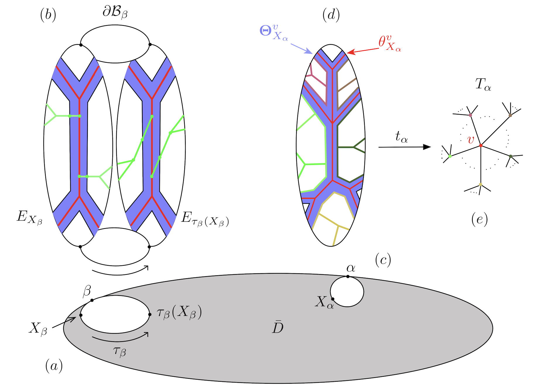
Figure 1 is a cartoon of the bundle $\bar{E}$ over the truncated Teichmüller disk $\bar{D}$. We have tried to highlight some of the key features of $\bar{E}$ which are relevant to this paper.

• (a)

  The stabilizer of a horoball based at a point $\beta\in\mathcal{P}$ is virtually cyclic, generated by a multitwist $\tau_{\beta}$ acting as a parabolic on $D$. The base point $X_{\beta}$ on the horocycle based at $\beta$ and its image are shown.

• (b)

  The bundle over the boundary horocycle based at $\beta$ is shown. This is the universal cover, $\partial\mathcal{B}_{\beta}$, of a graph manifold which is the mapping torus of $\tau_{\beta}$. Two fibers $E_{X_{\beta}}$ and $E_{\tau_{\beta}(X_{\beta})}$ are shown with the effect on a part of a spine (in green) in some other direction illustrating the sheering in strips after applying $\tau_{\beta}$.

• (c)

  This is another horoball in some direction $\alpha$, with the chosen basepoint $X_{\alpha}$ and its horocycle $\partial B_{\alpha}$.

• (d)

  The spine $\theta^{v}_{X_{\alpha}}$ in direction $\alpha$ is shown in red, corresponding to a vertex $v\in T_{\alpha}$. The thickened spine ${\bf\Theta}^{v}_{X_{\alpha}}$ is indicated in lavender. Spines for vertices of $T_{\alpha}$ adjacent to $v$ meet ${\bf\Theta}^{v}_{X_{\alpha}}$ along lines in $\partial{\bf\Theta}^{v}_{X_{\alpha}}$ and are shown in various other colors.

• (e)

  The restriction of $t_{\alpha}\colon E\to T_{\alpha}$ to $E_{X_{\alpha}}$ collapses each spine $\theta^{w}_{X_{\alpha}}$ or strip in direction $\alpha$ to the corresponding vertex $w$ or edge the Bass-Serre tree $T_{\alpha}$. The space $\hat{E}$ is formed by collapsing $\mathcal{B}_{\alpha}$ to $T_{\alpha}$ via $t_{\alpha}$.

Here we briefly recall some basic facts about the setup above proved in [DDLS21] as well as some useful coarse geometric facts. The first fact is the following; see [DDLS21, Lemma 3.4].

Every connected graph can be made into a geodesic metric space by locally isometrically identifying each edge with a unit interval. We will need the following well-known result (for a proof of this version, see [DDLS21, Proposition 2.1]).

The following criterion for a graph to be a quasi-tree is well-known, and an easy consequence of Manning’s bottleneck criterion [Man05]. We include a proof for completeness.

We end with a few definitions from coarse geometry which may not be completely standard, but will appear in the next two sections. Given two metrics $d$ and $d^{\prime}$ on a set $X$, we say that $d$ is coarsely bounded by $d^{\prime}$ if there exists a monotone function $N\colon[0,\infty)\to[0,\infty)$ so that $d(x,y)\leq N(d^{\prime}(x,y))$, for all $x,y\in X$. If $d$ is coarsely bounded by $d^{\prime}$ and $d^{\prime}$ is coarsely bounded by $d$, we say that $d$ and $d^{\prime}$ are coarsely equivalent. An isometric action of a group $H$ on a metric space $Y$ is metrically proper if for any $R>0$ and any point $y\in Y$, there are at most finitely many elements $h\in H$ for which $h\cdot B(y,R)\cap B(y,R)\neq\emptyset$. For proper geodesic spaces, this is equivalent to acting properly discontinuously. If there exists $y,R$ so that $H\cdot B(y,R)=Y$, then we say that the action is cobounded, and for proper geodesic metric spaces this is equivalent to acting cocompactly.

For each $v\in\mathcal{V}$, we will use ideas from work-in-progress of the fourth author with Hagen, Russell, and Spriano [HRSS21] to define a map

$$\lambda^{v}\colon{\bf\Theta}^{v}\rightarrow\mathcal{K}^{v},$$

where $\mathcal{K}^{v}$ is a discrete set quasi-isometric to $\mathbb{R}$. The key properties of this map are given by the next proposition. We note that the proposition and Lemma 3.6 can be used as black-boxes (in particular, the definitions of $\lambda^{v}$ and $\mathcal{K}^{v}$ are never used after we prove those results).

The sets $\ell_{x,\alpha}$ in item (2) are certain lines whose significance is explained below.

To explain the proof of the proposition, it is useful to review some background on graph manifolds, which we do now.

Recall that a graph manifold is a $3$–manifold that contains a canonical finite union of tori (up to isotopy), so that cutting along the tori produces a disjoint union of Seifert fibered $3$–manifolds, called the Seifert pieces. Seifert fibered $3$–manifolds are compact $3$–manifolds foliated by circle leaves; see [JS79].

The universal cover of a graph manifold decomposes into a union of universal covers of the Seifert pieces glued together along $2$–planes (covering the tori). The decomposition is dual to a tree, and the universal covers of the Seifert pieces are the vertex spaces. For any Seifert fibered space, its universal cover is foliated by lines, the lift of the foliation by circles, and we refer to the leaves simply as lines in the universal cover.

Next we describe the specific graph manifolds that are relevant for our purposes.

Let $G_{\alpha}<G$ denote the stabilizer of $B_{\alpha}$, for each $\alpha\in\mathcal{P}$. This has a finite index cyclic subgroup $G_{\alpha}^{0}$ generated by a multitwist, $\langle\tau_{\alpha}\rangle=G_{\alpha}^{0}<G_{\alpha}$; see e.g. [DDLS21, §2.9]. The preimage of $G_{\alpha}$ in $\Gamma$ is the $\pi_{1}S$–extension group $\Gamma_{\alpha}$ of $G_{\alpha}$, and we likewise denote by $\Gamma_{\alpha}^{0}<\Gamma_{\alpha}$ the extension group of $G_{\alpha}^{0}$. The action of $\Gamma_{\alpha}$ on $\partial\mathcal{B}_{\alpha}$ is cocompact, and $\partial\mathcal{B}_{\alpha}/\Gamma_{\alpha}$ has a finite sheeted (orbifold) covering by $\partial\mathcal{B}_{\alpha}/\Gamma_{\alpha}^{0}$, which is the graph manifold mentioned in the introduction.

Consider the surface $S$ with the flat metric $q_{X_{\alpha}}$, so that $(S,X_{\alpha},q_{X_{\alpha}})=E_{X_{\alpha}}/\pi_{1}S$. The multitwist $\tau_{\alpha}$ is an affine map that preserves the cylinders in direction $\alpha$, acting as a power of a Dehn twist in each cylinder and as the identity on their boundaries. The union of the boundaries of the cylinders are spines (deformation retracts) for the subsurfaces that are the complements of the twisting curves (core curves of the cylinders). Consequently, $\tau_{\alpha}$ is the identity on these spines. The homeomorphism $\tau_{\alpha}$ induces a homeomorphism on the subsurface obtained by cutting open $S$ along a core curve of each cylinder. Each such induced homeomorphism is the identity on the corresponding spine, and is thus isotopic to the identity relative to the spine; see Figure 2. The mapping torus of each subsurface is a product of the subsurface times a circle, and embeds in the the mapping torus $\partial\mathcal{B}_{\alpha}/\Gamma_{\alpha}^{0}$ of $\tau_{\alpha}$. These sub-mapping tori are the Seifert pieces for the graph manifold structure on $\partial\mathcal{B}_{\alpha}/\Gamma_{\alpha}^{0}$.

The lifted graph manifold decomposition of $\partial\mathcal{B}_{\alpha}$ corresponds to $T_{\alpha}$. That is, for each $v\in T_{\alpha}^{(0)}$, there is a vertex space contained in ${\bf\Theta}^{v}$ and containing $\theta^{v}$. In fact, with respect to the covering group, ${\bf\Theta}^{v}$ is an invariant, bounded neighborhood of the vertex space and $\theta^{v}$ is an equivariant deformation retraction of that space. We let $\Gamma^{v}<\Gamma_{\alpha}$ denote the stabilizer of ${\bf\Theta}^{v}$ in $\Gamma_{\alpha}$ and $\Gamma^{v0}<\Gamma_{\alpha}^{0}$ the stabilizer in $\Gamma_{\alpha}^{0}$. The suspension flow on the mapping torus $\partial\mathcal{B}_{\alpha}/\Gamma_{\alpha}^{0}$ restricted to each quotient of the spine bundle, $\theta^{v}/\Gamma^{v0}$, defines circle leaves of the corresponding Seifert piece; that is, flow lines through any point on the $\theta^{v}/\Gamma^{v0}$ are precisely the circle leaves. In the universal covering $\partial\mathcal{B}_{\alpha}$, the lifted flowline through a point $x\in\partial\mathcal{B}_{\alpha}$ is a lifted horocycle, $\ell_{x,\alpha}=D_{x}\cap\partial\mathcal{B}_{\alpha}$. Thus, for any vertex $v$ and any $x\in\theta^{v}$, $\ell_{x,\alpha}$ is a line for the vertex space corresponding to $v$. We note that not only does $\Gamma^{v0}$ preserve this set of lines, but so does $\Gamma^{v}$.

For any $x\in\theta^{v}$, the stabilizer in $\Gamma^{v0}$ of $\ell_{x,\alpha}$ is generated by a lift $g_{v}$ of $\tau_{\alpha}$. Therefore, the quotient ${\bf\Theta}^{v}/\Gamma^{v0}$ is homeomorphic to a product, ${\bf\Theta}^{v}_{X}/\pi_{1}S^{v}\times S^{1}$, where $\pi_{1}S^{v}$ is the stabilizer of $v$ in $\pi_{1}S<\Gamma$ and $X\subset\partial B_{\alpha}$ is any point. Indeed, there is a deformation retraction to $\theta^{v}/\Gamma^{v0}=\theta^{v}_{X}/\pi_{1}S^{v}\times S^{1}$. If we do not care about the particular point $X$ over which we take the fiber, we simply write $S^{v}$ for the surface ${\bf\Theta}^{v}_{X}/\pi_{1}S^{v}$, so that ${\bf\Theta}^{v}/\Gamma^{v0}\cong S^{v}\times S^{1}$. Since $E_{X}$ is a copy of the universal cover of $S$, we can consider $S^{v}$ as a subsurface of $S$ (embedded on the interior) and $\pi_{1}S^{v}$ is its fundamental group inside $\pi_{1}S$ (up to conjugacy).

The product structure $S^{v}\times S^{1}\cong{\bf\Theta}^{v}/\Gamma^{v0}$ can be chosen so that ${\bf\Theta}^{v}/\Gamma^{v0}\to{\bf\Theta}^{v}/\Gamma$ is an orbifold cover sending circles to circles making ${\bf\Theta}^{v}/\Gamma^{v}$ into a Seifert fibered orbifold (some of the Seifert fibers may be part of the orbifold locus) that also (orbifold)-fibers over the circle (with finite order monodromy). Write ${\bf\Theta}^{v}/\Gamma^{v}\to\mathcal{O}^{v}$ for the Seifert fibration to the quotient $2$–orbifold. Further write

$$\nu^{v}\colon\Gamma^{v}\to\pi_{1}^{orb}(\mathcal{O}^{v})$$

for the induced homomorphism of the Seifert fibration and

$$\phi^{v}\colon\Gamma^{v}\to\mathbb{Z}$$

for the induced homomorphism from the fibration over the circle. Because $g_{v}$ acts as translation on the line $\ell_{x,\alpha}$ for $x\in\theta^{v}$, it represents a loop that traverses a circle in the Seifert fibration, which is thus also a suspension flowline for the fibration over the circle. Thus we have $\nu^{v}(g_{v})=0$ and $\phi^{v}(g_{v})\neq 0$. To complete the picture, we note that restricting $S^{v}\times S^{1}\cong{\bf\Theta}^{v}/\Gamma^{v0}\to{\bf\Theta}^{v}/\Gamma^{v}\to\mathcal{O}^{v}$ to $S^{v}$ defines an orbifold covering $S^{v}\to\mathcal{O}^{v}$.

References

- [ABD21] Carolyn Abbott, Jason Behrstock, and Matthew Gentry Durham. Largest acylindrical actions and Stability in hierarchically hyperbolic groups. Trans. Amer. Math. Soc. Ser. B, 8:66–104, 2021.
- [ABO19] Carolyn Abbott, Sahana H. Balasubramanya, and Denis Osin. Hyperbolic structures on groups. Algebr. Geom. Topol., 19(4):1747–1835, 2019.
- [Ahl66] Lars V. Ahlfors. Fundamental polyhedrons and limit point sets of Kleinian groups. Proc. Nat. Acad. Sci. U.S.A., 55:251–254, 1966.
- [BBKL20] Mladen Bestvina, Kenneth Bromberg, Autumn E. Kent, and Christopher J. Leininger. Undistorted purely pseudo-Anosov groups. J. Reine Angew. Math., 760:213–227, 2020.
- [BHMS20] Jason Behrstock, Mark F. Hagen, A. Martin, and A. Sisto. A combinatorial take on hierarchical hyperbolicity and applications to quotients of mapping class groups. preprint, arXiv:2005.00567, 2020.
- [BHS17a] Jason Behrstock, Mark F. Hagen, and Alessandro Sisto. Asymptotic dimension and small-cancellation for hierarchically hyperbolic spaces and groups. Proc. Lond. Math. Soc. (3), 114(5):890–926, 2017.
- [BHS17b] Jason Behrstock, Mark F. Hagen, and Alessandro Sisto. Hierarchically hyperbolic spaces, I: Curve complexes for cubical groups. Geom. Topol., 21(3):1731–1804, 2017.
- [BHS19] Jason Behrstock, Mark Hagen, and Alessandro Sisto. Hierarchically hyperbolic spaces II: Combination theorems and the distance formula. Pacific J. Math., 299(2):257–338, 2019.
- [BHS21] Jason Behrstock, Mark F. Hagen, and Alessandro Sisto. Quasiflats in hierarchically hyperbolic spaces. Duke Math. J., 170(5):–, 2021.
- [BL18] Anja Bankovic and Christopher J. Leininger. Marked-length-spectral rigidity for flat metrics. Trans. Amer. Math. Soc., 370(3):1867–1884, 2018.
- [Bow93] B. H. Bowditch. Geometrical finiteness for hyperbolic groups. J. Funct. Anal., 113(2):245–317, 1993.
- [Bow13] Brian H. Bowditch. Coarse median spaces and groups. Pacific J. Math., 261(1):53–93, 2013.
- [Bow18] Brian H. Bowditch. Large-scale rigidity properties of the mapping class groups. Pacific J. Math., 293(1):1–73, 2018.
- [CLM12] Matt T. Clay, Christopher J. Leininger, and Johanna Mangahas. The geometry of right-angled Artin subgroups of mapping class groups. Groups Geom. Dyn., 6(2):249–278, 2012.
- [DDLS21] Spencer Dowdall, Matthew G. Durham, Christopher J. Leininger, and Allesandro Sisto. Extensions of Veech groups I: A hyperbolic action. arXiv preprint arXiv:2006.16425v2, 2021.
- [DELS18] Moon Duchin, Viveka Erlandsson, Christopher J. Leininger, and Chandrika Sadanand. You can hear the shape of a billiard table: Symbolic dynamics and rigidity for flat surfaces. Preprint, to appear in Comment. Math. Helv., 2018.
- [DGO17] F. Dahmani, V. Guirardel, and D. Osin. Hyperbolically embedded subgroups and rotating families in groups acting on hyperbolic spaces. Mem. Amer. Math. Soc., 245(1156):v+152, 2017.
- [DHS17] Matthew Gentry Durham, Mark F. Hagen, and Alessandro Sisto. Boundaries and automorphisms of hierarchically hyperbolic spaces. Geom. Topol., 21(6):3659–3758, 2017.
- [DMS20] Matthew G Durham, Yair N Minsky, and Alessandro Sisto. Stable cubulations, bicombings, and barycenters. arXiv preprint arXiv:2009.13647, 2020.
- [DT15] Matthew Gentry Durham and Samuel J. Taylor. Convex cocompactness and stability in mapping class groups. Algebr. Geom. Topol., 15(5):2839–2859, 2015.
- [EF97] David B. A. Epstein and Koji Fujiwara. The second bounded cohomology of word-hyperbolic groups. Topology, 36(6):1275–1289, 1997.
- [Far98] B. Farb. Relatively hyperbolic groups. Geom. Funct. Anal., 8(5):810–840, 1998.
- [FM00] Benson Farb and Lee Mosher. On the asymptotic geometry of abelian-by-cyclic groups. Acta Math., 184(2):145–202, 2000.
- [FM02a] Benson Farb and Lee Mosher. Convex cocompact subgroups of mapping class groups. Geom. Topol., 6:91–152, 2002.
- [FM02b] Benson Farb and Lee Mosher. The geometry of surface-by-free groups. Geometric & Functional Analysis GAFA, 12(5):915–963, 2002.
- [GM91] F.P. Gardiner and H.A. Masur. Extremal length geometry of Teichmüller space. Complex Variables Theory Appl., 16(2-3):209–237, 1991.
- [Gre66] L. Greenberg. Fundamental polyhedra for kleinian groups. Ann. of Math. (2), 84:433–441, 1966.
- [Ham] Ursula Hamenstädt. Word hyperbolic extensions of surface groups. Preprint, arXiv:math.GT/0505244.
- [HHP20] Thomas Haettel, Nima Hoda, and Harry Petyt. Coarse injectivity, hierarchical hyperbolicity, and semihyperbolicity. arXiv preprint arXiv:2009.14053, 2020. To appear in Geom. Topol.
- [HO13] Michael Hull and Denis Osin. Induced quasicocycles on groups with hyperbolically embedded subgroups. Algebr. Geom. Topol., 13(5):2635–2665, 2013.
- [HRSS21] Mark F. Hagen, Jacob Russell, Alessandro Sisto, and Davide Spriano. Equivariant hierarchically hyperbolic structures for 3-manifold groups via quasimorphisms. In preparation, 2021.
- [JS79] William H. Jaco and Peter B. Shalen. Seifert fibered spaces in -manifolds. Mem. Amer. Math. Soc., 21(220):viii+192, 1979.
- [KL97] Michael Kapovich and Bernhard Leeb. Quasi-isometries preserve the geometric decomposition of Haken manifolds. Invent. Math., 128(2):393–416, 1997.
- [KL07] Autumn E. Kent and Christopher J. Leininger. Subgroups of mapping class groups from the geometrical viewpoint. In In the tradition of Ahlfors-Bers. IV, volume 432 of Contemp. Math., pages 119–141. Amer. Math. Soc., Providence, RI, 2007.
- [KL08a] Autumn E. Kent and Christopher J. Leininger. Shadows of mapping class groups: capturing convex cocompactness. Geom. Funct. Anal., 18(4):1270–1325, 2008.
- [KL08b] Autumn E. Kent and Christopher J. Leininger. Uniform convergence in the mapping class group. Ergodic Theory Dynam. Systems, 28(4):1177–1195, 2008.
- [KL12] Ilya Kapovich and Anton Lukyanenko. Quasi-isometric co-Hopficity of non-uniform lattices in rank-one semi-simple Lie groups. Conform. Geom. Dyn., 16:269–282, 2012.
- [Kob12] Thomas Koberda. Right-angled Artin groups and a generalized isomorphism problem for finitely generated subgroups of mapping class groups. Geom. Funct. Anal., 22(6):1541–1590, 2012.
- [Loa21] Christopher Loa. Free products of abelian groups in mapping class groups. arXiv preprint arXiv:2103.05144, 2021.
- [LR06] C. J. Leininger and A. W. Reid. A combination theorem for Veech subgroups of the mapping class group. Geom. Funct. Anal., 16(2):403–436, 2006.
- [Man05] Jason Fox Manning. Geometry of pseudocharacters. Geom. Topol., 9:1147–1185, 2005.
- [Mar74] Albert Marden. The geometry of finitely generated kleinian groups. Ann. of Math. (2), 99:383–462, 1974.
- [Mas70] Bernard Maskit. On boundaries of Teichmüller spaces and on Kleinian groups. II. Ann. of Math. (2), 91:607–639, 1970.
- [Min96a] Yair N. Minsky. Extremal length estimates and product regions in Teichmüller space. Duke Math. J., 83(2):249–286, 1996.
- [Min96b] Yair N. Minsky. Quasi-projections in Teichmüller space. J. Reine Angew. Math., 473:121–136, 1996.
- [MM99] H.A. Masur and Y.N. Minsky. Geometry of the complex of curves. I. Hyperbolicity. Invent. Math., 138(1):103–149, 1999.
- [MM00] H.A. Masur and Y. N. Minsky. Geometry of the complex of curves. II. Hierarchical structure. Geom. Funct. Anal., 10(4):902–974, 2000.
- [Mos03] Lee Mosher. Fiber respecting quasi-isometries of surface group extensions. preprint arXiv:math/0308067, 2003.
- [Mos06] Lee Mosher. Problems in the geometry of surface group extensions. In Problems on mapping class groups and related topics, volume 74 of Proc. Sympos. Pure Math., pages 245–256. Amer. Math. Soc., Providence, RI, 2006.
- [MS12] Mahan Mj and Pranab Sardar. A combination theorem for metric bundles. Geom. Funct. Anal., 22(6):1636–1707, 2012.
- [MT02] Howard Masur and Serge Tabachnikov. Rational billiards and flat structures. In Handbook of dynamical systems, Vol. 1A, pages 1015–1089. North-Holland, Amsterdam, 2002.
- [MW95] H.A. Masur and M. Wolf. Teichmüller space is not Gromov hyperbolic. Ann. Acad. Sci. Fenn. Ser. A I Math., 20(2):259–267, 1995.
- [Raf14] Kasra Rafi. Hyperbolicity in Teichmüller space. Geom. Topol., 18(5):3025–3053, 2014.
- [RST18] Jacob Russell, Davide Spriano, and Hung Cong Tran. Convexity in hierarchically hyperbolic spaces. arXiv preprint arXiv:1809.09303, 2018. To appear in Algebr. Geom. Topol.
- [Run20] Ian Runnels. Effective generation of right-angled artin groups in mapping class groups. arXiv preprint arXiv:2004.13585, 2020.
- [Rus21] Jacob Russell. Extensions of multicurve stabilizers are hierarchically hyperbolic. arXiv preprint arXiv:2107.14116, 2021.
- [Sch95] Richard Evan Schwartz. The quasi-isometry classification of rank one lattices. Inst. Hautes Études Sci. Publ. Math., (82):133–168 (1996), 1995.
- [Sis16] Alessandro Sisto. Quasi-convexity of hyperbolically embedded subgroups. Math. Z., 283(3-4):649–658, 2016.
- [Sis19] Alessandro Sisto. What is a hierarchically hyperbolic space? In Beyond hyperbolicity, volume 454 of London Math. Soc. Lecture Note Ser., pages 117–148. Cambridge Univ. Press, Cambridge, 2019.
- [Tan19] Robert Tang. Affine diffeomorphism groups are undistorted. preprint arXiv:1912.06537, 2019.
- [Thu86] W.P. Thurston. Geometry and topology of –manifolds. Princeton University Lecture Notes, online at http://www.msri.org/publications/books/gt3m, 1986.