Extracting the Lifetime of a Synthetic Two-Level System
Abstract
The Kerr Parametric Oscillator (KPO) is a nonlinear resonator system that is often described as a synthetic two-level system. In the presence of noise, the system switches between two states via a fluctuating trajectory in phase space, instead of following a straight path. The presence of such fluctuating trajectories makes it hard to establish a precise count, or even a useful definition, of the “lifetime” of the state. Addressing this issue, we compare several rate counting methods that allow to estimate a lifetime for the levels. In particular, we establish that a peak in the Allan variance of fluctuations can also be used to determine the levels’ lifetime. Our work provides a basis for characterizing KPO networks for simulated annealing where an accurate determination of the state lifetime is of fundamental importance.
Synthetic two level systems (TLSs) generated in driven nonlinear resonators have recently caught a significant attention in the physics community Gottesman et al. (2001); Devoret and Schoelkopf (2013). A particularly prominent example is the Kerr Parametric Oscillator (KPO, also known as parametron) Mahboob and Yamaguchi (2008); Wilson et al. (2010); Eichler et al. (2011, 2018); Gieseler et al. (2012); Lin et al. (2014); Puri et al. (2017); Nosan et al. (2019); Frimmer et al. (2019); Grimm et al. (2019); Puri et al. (2019); Miller et al. (2019a); Ryvkine and Dykman (2006) whose potential energy is pumped at frequency close to twice its resonance frequency , i.e. at . If the modulation strength exceeds a threshold , the device responds with oscillations locked to within a certain detuning range. This well-known “period doubling” of the response relative to the pump gives rise to two stable “phase states” with the same amplitude but separated by a phase difference of . The phase states can be used to encode the two polarization states (up/down) of a classical spin. This analogy leads to the idea of using networks of coupled KPOs to build noisy intermediate-scale quantum (NISQ) machines Preskill (2018); Albash and Lidar (2018). These machines can simulate the dynamics of mathematical problems that overwhelm traditional computers, such as the ground state of an Ising Hamiltonian Ising (1925); Goto et al. (2018); Rota et al. (2019); Heim et al. (2015); Mahboob et al. (2016); Inagaki et al. (2016a); Goto (2016); Bello et al. (2019); Okawachi et al. (2020); Calvanese Strinati et al. (2019), or of other complex systems that can be mapped onto the same framework Lucas (2014); Nigg et al. (2017); Inagaki et al. (2016b); Goto et al. (2019); Honjo et al. (2021).
An important quantity for many applications of TLSs is their lifetime Krantz et al. (2019). It is the typical time spent on a level before the interaction with an environment induces a (seemingly) spontaneous “jump” from one state to the other. The rates of environmental noise-induced switching have previously been investigated for different systems, such as trapped electrons Lapidus et al. (1999), cold atoms Kim et al. (2005), micromechanical systems Aldridge and Cleland (2005); Chan and Stambaugh (2007); Venstra et al. (2013) and analog electronic circuits Luchinsky et al. (1999).
The situation is more subtle for a KPO. Here, the synthetic levels are formed by coherent bosonic states forming attractors in phase space. These attractors are not separated by an energy gap but by a phase gap Frimmer et al. (2019). When switches occur on a slow timescale (relative to the resonator relaxation time) and follow narrow channels in phase space, the fluctuations are termed “weak”. Such a setting allows for situations with negligible backaction where the fluctuations during a single switch can be observed. Currently, however, there exist very few studies of the fascinating physics unfolding during individual switches Chan et al. (2008); Mahboob et al. (2014); Dykman et al. (1998); Chan and Stambaugh (2007).
In this work, we study a classical micromechanical KPO and investigate its switching rates in the presence of weak fluctuations. We invoke and compare several methods previously used to characterize the rates of charge and parity state switching in Cooper pair boxes and superconducting qubits Serniak et al. (2018, 2019). Furthermore, we propose a method to calculate the switching rate that is based on the Allan variance of the resonator displacement Van Vliet and Handel (1982). In the final part of the paper, we compare all methods and find good agreement between several (but not all) of them.
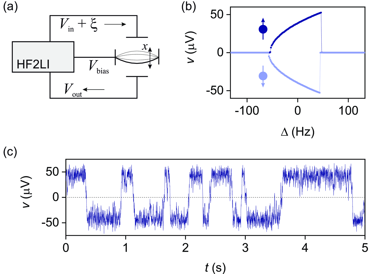
Our KPO consists of a micro-electromechanical resonator (MEMS) in a room-temperature setup schematically shown in Fig. 1(a). The resonator is a doubly-clamped beam, with the length of , width , and in thickness with a lumped mass of 25.4 ng made from highly-doped single crystal silicon and fabricated in a wafer-scale encapsulation process Yang et al. (2016). Electrodes on both sides separated from the conducting beam with a gap enable capacitive driving and sensitive detection of oscillations in the presence of a bias voltage, Miller et al. (2019b). We use a Zurich Instruments HF2LI lock-in amplifier to apply the driving voltage and to measure the resonator displacement with quadrature amplitudes and . For convenience, we drop the proportionality factor between and and identify in the following Nosan et al. (2019).
Our mechanical resonator can be described by the nonlinear equation of motion (in units of the measured electrical signal)
| (1) |
Here, dots indicate time derivatives, is the resonance frequency, the coefficient of the Duffing nonlinearity, the resonator relaxation rate, and the quality factor of the resonator. The potential energy term () is pumped with the parametric modulation depth at the angular frequency , and where is the voltage threshold for parametric oscillations for the case (demodulation frequency). The potential modulation arises because the electrostatic force due to pulls the beam closer towards one electrode. The force is nonlinear, i.e., it grows stronger for small beam-electrode distances, which corresponds to a change in the overall spring constant that the beam experiences. As a consequence, the drive generates small frequency variations . The force term in Eq. 1 represents a fluctuating thermal bath [see Supplemental Material (SM) for details].
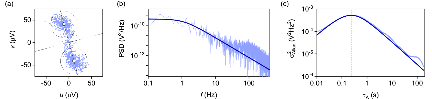
Figure 1(b) shows the -quadrature response of the resonator during two sweeps of from positive to negative detuning . Close to , the response jumps from to , marking a bifurcation point of the underlying nonlinear system. At the bifurcation, the resonator experiences a spontaneous symmetry breaking, also known as a period-doubling bifurcation or a discrete time-translation breaking Landau and Lifshitz (1976); Heugel et al. (2019). At this point, the resonator jumps to a positive or negative response with equal probability. The two responses belong to stable attractors ( and ) with opposite phases, i.e., (and ) Calvanese Strinati et al. (2019); Lifshitz (2009); Dykman and Krivoglaz (1979); Papariello et al. (2016).
To study switching between the phase states of our KPO, we apply white electrical noise characterized by a standard deviation (over a bandwidth of ) that causes the state of the resonator to fluctuate around its initial solution. If the fluctuations are large enough, they will occasionally carry the resonator across the threshold in the middle between the phase states. The resonator is then captured by the opposite attractor, corresponding to a switch of the synthetic TLS. Several such processes can be observed in Fig. 1(c). From this observation, it appears natural to attribute a lifetime to the inverse switching rate, . However, calculating the switching rate is not straightforward due to the fluctuating trajectory.
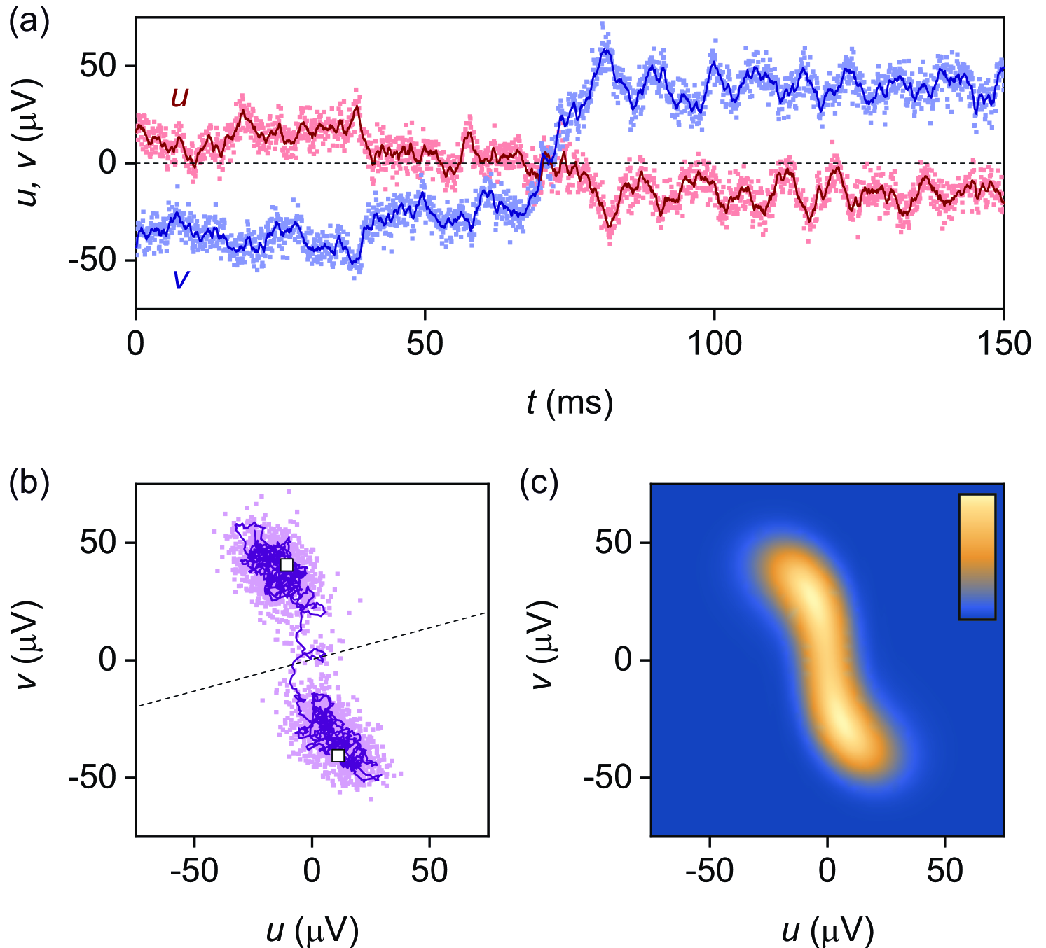
For a deeper understanding of the system’s transient behaviour during switching events, we perform measurements with a high temporal resolution. In Fig. 2(a)-(b), we display a narrow time segment before, during, and after a single switch. We find many data points in the unstable zone between the two phase states. A 10-point moving average filter helps to visualize the trajectory of the system during the transition. The total switching time is roughly , much longer than the lock-in integration time of and the moving-average filter time of . The measurement error of each data point is , in agreement with the measured point-to-point fluctuations, but significantly smaller than the fluctuations visible on the scale.
Our observation depicted in Fig. 2 demonstrates that activated switches between the phase states are not deterministic, but include prominent random elements. For instance, in the phase-space representation of the switch in Fig. 2(b) we can clearly see that the system performs a winding path close to the origin. In our device, the fluctuations generally have a slight preference for counter-clockwise rotations around the phase states and clockwise ones around the origin. This can be explained by the combination of the drive and the nonlinearity, which leads to an effective detuning of the fluctuations from the lock-in amplifier clock Heugel et al. (2021). In the corresponding Fokker-Planck steady-state calculation presented in Fig. 2(c), we therefore find a channel with a significant probability density between the phase states.
These visualizations of the fluctuating trajectories expose a fundamental problem in estimating the lifetime : since transitions follow no straight lines, they can cross any point in phase space multiple times during a single switching event. An example of this can be observed in Fig. 2(b), where the averaged (dark) trajectory crosses the dotted threshold line from bottom to top, describes a clockwise winding that traverses back across the threshold, and finally crosses the line a third time before completing the switch. A simple counting algorithm will in this case register three crossing events during a single switch. In general, any counting method based on a simple threshold (such as a line) will therefore overestimate the switching number during the full time , and therefore also . This problem has been known since a long time.
The problem of overestimating the switching count can be reduced by defining multiple thresholds that have to be crossed in a particular order to constitute an event. In Fig. 3(a), we demonstrate this with the example of two circles in phase space. The count is increased by one each time a circular threshold is left and the opposing circle is entered. This method is less sensitive to small fluctuations, but it requires a subjective measure that impacts the estimated , in our case the radii of the circular thresholds. Calibrating the measured switching rate as a function of the radius helps to reduce this degree of arbitrariness (see SM), but it cannot be removed entirely.
To avoid overcounting and subjective dependencies, it is desirable to extract from a method that does not require thresholds at all. Interestingly, the parity lifetime of superconducting qubits can be determined via their charge-parity power spectral density (PSD) Dutta and Horn (1981); Ristè et al. (2013); Serniak et al. (2018). Assuming that the switching is dominated by telegraph noise, the PSD of of our KPO can be fitted to a Lorentzian function,
| (2) |
where the lifetime corresponds to the characteristic time scale between level switching events, and is a constant related to the measurement fidelity Ristè et al. (2013). In this case, the lifetime or the switching rate is related to the width of the spectral peak in the frequency domain Demtröder (1973). To make the estimate quantitative in Fig. 3(b), we fit the measured displacement power spectral density with Eq. (2), yielding a third estimation for lifetime. The method can also be applied after a Fourier transform by fitting the sliding average autocorrelation with the function under the assumption of stationarity and ergodicity (not shown).
Crucially, the autocorrelation is intimately related to the Allan variance (see SM for the derivation). Originally invented to characterize the fidelity of clocks, the Allan variance measures the frequency fluctuations of a resonator as a function of integration time . As we are interested in the time over which the typical fluctuations of (or ) of our KPO are maximal, we apply the Allan variance formalism Allan (1966) to the measured values,
| (3) |
In this notation,
| (4) |
are sums over the measured values (or values) and denotes the mean over , running from to , where is the total number of data points and is the sampling time. Assuming that the signal is dominated by telegraph-like switching with lifetime and amplitude , we obtain Van Vliet and Handel (1982):
| (5) |
Hence, the maximum of should occur around the value . In Fig. 3(c), we indeed find a peak at the expected value, yielding . In contrast to the PSD method, the Allan variance method does not necessarily require a fitting process, as the peak can be read off directly and is easy to interpret even in the presence of noise.
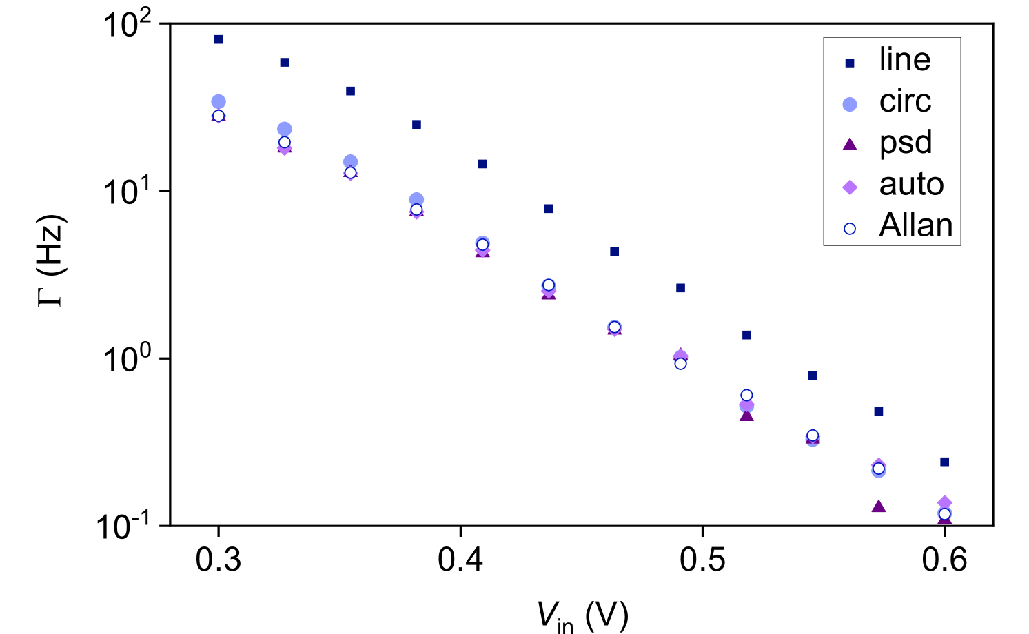
We compare the results of the different methods in Fig. 4. We find excellent agreement between four out of five of the methods for values of varying over more than two orders of magnitude. The only method that we wish to discard from this comparison is the simple line threshold approach, which consistently overestimates the count rate as expected from the discussion above. The method using two circles for thresholding overestimates slightly for , where the separation between the attractors is small and the “clouds” start to overlap significantly, cf. the example in Fig. 3(a). Additional comparison as a function of the noise strength can be found in SM.
We emphasize that there is no fundamental reason why the estimators we obtain should be identical at all. The surprisingly good agreement between most of the estimators confirms that the notion of a lifetime is useful to characterize the switching between phase states in a KPO, where a parametric pump generates a synthetic potential landscape Heugel et al. (2019). This approach may be useful in other systems where multi-stable potentials in dimensions higher than one are present, such as three-dimensional protein folding or other chemical reactions. For advanced applications in the future, the resonator networks could be realized through bilinear, resonant coupling of several KPOs Bello et al. (2019); Heugel et al. (2021) (see SM for details). For MEMS such as those studied here, bilinear coupling can be achieved in multiple ways, such as pairwise capacitive, inductive, optical, or mechanical coupling, or indirect all-to-all coupling through a separate radio-frequency cavity.
Data availability statement: The data that support the findings of this study are available from the corresponding author upon reasonable request.
The authors have no conflicts to disclose.
I Supplementary Material
The supplementary material contains theory derivations for the probability density, the Allan variance, and the autocorrelation of telegraph noise, experimental demonstrations of the dependence of the extracted switching rate on the circle threshold radius and on the noise strength, and a short summary of various coupling methods for parametric oscillators.
Acknowledgments
Fabrication was performed in nano@Stanford labs, which are supported by the National Science Foundation (NSF) as part of the National Nanotechnology Coordinated Infrastructure under Award No. ECCS-1542152, with support from the Defense Advanced Research Projects Agency’s Precise Robust Inertial Guidance for Munitions (PRIGM) Program, managed by Ron Polcawich and Robert Lutwak. This work was further supported by the Swiss National Science Foundation through grants (CRSII5_177198/1) and (PP00P2 190078), and by the Deutsche Forschungsgemeinschaft (DFG) - project number 449653034.
References
- Gottesman et al. (2001) D. Gottesman, A. Kitaev, and J. Preskill, Phys. Rev. A 64, 012310 (2001).
- Devoret and Schoelkopf (2013) M. H. Devoret and R. J. Schoelkopf, Science 339, 1169 (2013).
- Mahboob and Yamaguchi (2008) I. Mahboob and H. Yamaguchi, Nature Nanotechnology 3, 275 (2008).
- Wilson et al. (2010) C. M. Wilson, T. Duty, M. Sandberg, F. Persson, V. Shumeiko, and P. Delsing, Phys. Rev. Lett. 105, 233907 (2010).
- Eichler et al. (2011) A. Eichler, J. Chaste, J. Moser, and A. Bachtold, Nano Letters 11, 2699 (2011).
- Eichler et al. (2018) A. Eichler, T. L. Heugel, A. Leuch, C. L. Degen, R. Chitra, and O. Zilberberg, Applied Physics Letters 112, 233105 (2018).
- Gieseler et al. (2012) J. Gieseler, B. Deutsch, R. Quidant, and L. Novotny, Phys. Rev. Lett. 109, 103603 (2012).
- Lin et al. (2014) Z. Lin, K. Inomata, K. Koshino, W. D. Oliver, Y. Nakamura, J. S. Tsai, and T. Yamamoto, Nature Communications 5, 4480 (2014).
- Puri et al. (2017) S. Puri, S. Boutin, and A. Blais, npj Quantum Information 3, 18 (2017).
- Nosan et al. (2019) Z. Nosan, P. Märki, N. Hauff, C. Knaut, and A. Eichler, Phys. Rev. E 99, 062205 (2019).
- Frimmer et al. (2019) M. Frimmer, T. L. Heugel, Z. Nosan, F. Tebbenjohanns, D. Hälg, A. Akin, C. L. Degen, L. Novotny, R. Chitra, O. Zilberberg, and A. Eichler, Phys. Rev. Lett. 123, 254102 (2019).
- Grimm et al. (2019) A. Grimm, N. E. Frattini, S. Puri, S. O. Mundhada, S. Touzard, M. Mirrahimi, S. M. Girvin, S. Shankar, and M. H. Devoret, Nature 584, 205 (2019).
- Puri et al. (2019) S. Puri, A. Grimm, P. Campagne-Ibarcq, A. Eickbusch, K. Noh, G. Roberts, L. Jiang, M. Mirrahimi, M. H. Devoret, and S. M. Girvin, Phys. Rev. X 9, 041009 (2019).
- Miller et al. (2019a) J. M. Miller, D. D. Shin, H.-K. Kwon, S. W. Shaw, and T. W. Kenny, Phys. Rev. Applied 12, 044053 (2019a).
- Ryvkine and Dykman (2006) D. Ryvkine and M. I. Dykman, Physical Review E 74, 061118 (2006).
- Preskill (2018) J. Preskill, Quantum 2, 79 (2018).
- Albash and Lidar (2018) T. Albash and D. A. Lidar, Rev. Mod. Phys. 90, 015002 (2018).
- Ising (1925) E. Ising, Zeitschrift für Physik 31, 253 (1925).
- Goto et al. (2018) H. Goto, Z. Lin, and Y. Nakamura, Scientific Reports 8, 7154 (2018).
- Rota et al. (2019) R. Rota, F. Minganti, C. Ciuti, and V. Savona, Phys. Rev. Lett. 122, 110405 (2019).
- Heim et al. (2015) B. Heim, T. F. Rønnow, S. V. Isakov, and M. Troyer, Science 348, 215 (2015).
- Mahboob et al. (2016) I. Mahboob, H. Okamoto, and H. Yamaguchi, Science Advances 2, e1600236 (2016).
- Inagaki et al. (2016a) T. Inagaki, K. Inaba, R. Hamerly, K. Inoue, Y. Yamamoto, and H. Takesue, Nature Photonics 10, 415 (2016a).
- Goto (2016) H. Goto, Scientific Reports 6, 21686 (2016).
- Bello et al. (2019) L. Bello, M. Calvanese Strinati, E. G. Dalla Torre, and A. Pe’er, Phys. Rev. Lett. 123, 083901 (2019).
- Okawachi et al. (2020) Y. Okawachi, M. Yu, J. K. Jang, X. Ji, Y. Zhao, B. Y. Kim, M. Lipson, and A. L. Gaeta, Nature Communications 11, 4119 (2020).
- Calvanese Strinati et al. (2019) M. Calvanese Strinati, L. Bello, A. Pe’er, and E. G. Dalla Torre, Phys. Rev. A 100, 023835 (2019).
- Lucas (2014) A. Lucas, Frontiers in Physics 2, 5 (2014).
- Nigg et al. (2017) S. E. Nigg, N. Lörch, and R. P. Tiwari, Science Advances 3 (2017), 10.1126/sciadv.1602273.
- Inagaki et al. (2016b) T. Inagaki, Y. Haribara, K. Igarashi, T. Sonobe, S. Tamate, T. Honjo, A. Marandi, P. L. McMahon, T. Umeki, K. Enbutsu, O. Tadanaga, H. Takenouchi, K. Aihara, K.-i. Kawarabayashi, K. Inoue, S. Utsunomiya, and H. Takesue, Science 354, 603 (2016b).
- Goto et al. (2019) H. Goto, K. Tatsumura, and A. R. Dixon, Science advances 5, eaav2372 (2019).
- Honjo et al. (2021) T. Honjo, T. Sonobe, K. Inaba, T. Inagaki, T. Ikuta, Y. Yamada, T. Kazama, K. Enbutsu, T. Umeki, R. Kasahara, et al., Science advances 7, eabh0952 (2021).
- Krantz et al. (2019) P. Krantz, M. Kjaergaard, F. Yan, T. P. Orlando, S. Gustavsson, and W. D. Oliver, Applied Physics Reviews 6, 021318 (2019).
- Lapidus et al. (1999) L. J. Lapidus, D. Enzer, and G. Gabrielse, Phys. Rev. Lett. 83, 899 (1999).
- Kim et al. (2005) K. Kim, M.-S. Heo, K.-H. Lee, H.-J. Ha, K. Jang, H.-R. Noh, and W. Jhe, Phys. Rev. A 72, 053402 (2005).
- Aldridge and Cleland (2005) J. S. Aldridge and A. N. Cleland, Phys. Rev. Lett. 94, 156403 (2005).
- Chan and Stambaugh (2007) H. B. Chan and C. Stambaugh, Phys. Rev. Lett. 99, 060601 (2007).
- Venstra et al. (2013) W. J. Venstra, H. J. Westra, and H. S. Van Der Zant, Nature communications 4, 1 (2013).
- Luchinsky et al. (1999) D. G. Luchinsky, R. S. Maier, R. Mannella, P. V. E. McClintock, and D. L. Stein, Phys. Rev. Lett. 82, 1806 (1999).
- Chan et al. (2008) H. B. Chan, M. I. Dykman, and C. Stambaugh, Phys. Rev. Lett. 100, 130602 (2008).
- Mahboob et al. (2014) I. Mahboob, M. Mounaix, K. Nishiguchi, A. Fujiwara, and H. Yamaguchi, Scientific Reports 4, 4448 (2014).
- Dykman et al. (1998) M. I. Dykman, C. M. Maloney, V. N. Smelyanskiy, and M. Silverstein, Phys. Rev. E 57, 5202 (1998).
- Serniak et al. (2018) K. Serniak, M. Hays, G. De Lange, S. Diamond, S. Shankar, L. Burkhart, L. Frunzio, M. Houzet, and M. Devoret, Physical review letters 121, 157701 (2018).
- Serniak et al. (2019) K. Serniak, S. Diamond, M. Hays, V. Fatemi, S. Shankar, L. Frunzio, R. Schoelkopf, and M. Devoret, Phys. Rev. Applied 12, 014052 (2019).
- Van Vliet and Handel (1982) C. M. Van Vliet and P. H. Handel, Physica A: Statistical Mechanics and its Applications 113, 261 (1982).
- Yang et al. (2016) Y. Yang, E. J. Ng, Y. Chen, I. B. Flader, and T. W. Kenny, Journal of Microelectromechanical Systems 25, 489 (2016).
- Miller et al. (2019b) J. M. Miller, N. E. Bousse, D. B. Heinz, H. J. K. Kim, H.-K. Kwon, G. D. Vukasin, and T. W. Kenny, Journal of Microelectromechanical Systems 28, 965 (2019b).
- Landau and Lifshitz (1976) L. Landau and E. Lifshitz, Mechanics, Butterworth-Heinemann (1976).
- Heugel et al. (2019) T. L. Heugel, M. Oscity, A. Eichler, O. Zilberberg, and R. Chitra, Phys. Rev. Lett. 123, 124301 (2019).
- Lifshitz (2009) M. C. Lifshitz, R. Cross, “Nonlinear dynamics of nanomechanical and micromechanical resonators,” in Reviews of Nonlinear Dynamics and Complexity (Wiley-VCH, 2009) pp. 1–52.
- Dykman and Krivoglaz (1979) M. Dykman and M. Krivoglaz, Sov. Phys. JETP 50, 30 (1979).
- Papariello et al. (2016) L. Papariello, O. Zilberberg, A. Eichler, and R. Chitra, Phys. Rev. E 94, 022201 (2016).
- Heugel et al. (2021) T. L. Heugel, O. Zilberberg, C. Marty, R. Chitra, and A. Eichler, arXiv preprint arXiv:2103.02625 (2021).
- Dutta and Horn (1981) P. Dutta and P. M. Horn, Rev. Mod. Phys. 53, 497 (1981).
- Ristè et al. (2013) D. Ristè, C. Bultink, M. Tiggelman, R. Schouten, K. Lehnert, and L. DiCarlo, Nature communications 4, 1 (2013).
- Demtröder (1973) W. Demtröder, Laser spectroscopy, Vol. 5 (Springer, 1973).
- Allan (1966) D. W. Allan, Proceedings of the IEEE 54, 221 (1966).