Extracting the number of type-B Goldstone modes and the dynamical critical exponent for a type of scale-invariant states

In the last decades, much attention has been paid to investigations into quantum critical phenomena QPT . In particular, significant effort has been made in achieving a long-term goal towards a complete classification of quantum phase transitions and quantum states of matter in one-dimensional quantum many-body systems wen ; pollmann1 . Historically, this may be dated back to the early work by Polyakov Popkov , who speculated that scale invariance implies conformal invariance. This speculation eventually led to the creation of conformal field theory Belavin , thus making it possible to classify all possible critical points in terms of central charge and conformal dimensions. Given a few counter-examples are known Hortacsu ; Strominger ; LeClair ; Zamolodchikov , it appears to be necessary to launch a systematic search for scale-invariant, but not conformally invariant, quantum states of matter.

Indeed, the presence of scale-invariant, but not conformally invariant, quantum states of matter strongly suggests that the current classification of quantum phase transitions and quantum states of matter is far from complete, even for those relevant to spontaneous symmetry breaking (SSB) anderson . As it turns out, highly degenerate ground states arising from SSB with type-B Goldstone modes (GMs) are scale-invariant FMGM ; golden ; LLspin1 , with the ${\rm SU}(2)$ Heisenberg ferromagnetic model being a paradigmatic example. In fact the highly degenerate ground states admit an exact singular value decomposition, thus exhibiting self-similarities underlying the ground state subspace. In other words, an abstract fractal is revealed, living in a Hilbert space, which may be characterized in terms of the fractal dimension, first introduced by Castro-Alvaredo and Doyon doyon for the ${\rm SU}(2)$ Heisenberg ferromagnetic states. A remarkable fact is that the fractal dimension may be identified with the number of type-B GMs FMGM ; golden , thus unveiling a deep connection between scale-invariant states and the counting rule of the GMs Watanabe . The establishment of the counting rule is largely based on an insightful observation made by Nambu nambu , culminating in the classification of type-A and type-B GMs.

In addition, our current understanding of quantum critical phenomena has been reshaped from the novel perspective of quantum information science nielsen ; amico . In particular, the entanglement entropy is demonstrated to be a powerful means for characterizing quantum phase transitions vidal ; Korepin ; cardy ; zhou . This in turn motivated the development of powerful tensor network representations to simulate quantum many-body systems itebd ; idmrg ; Orus ; ipeps ; frank ; corboz ; czarnik . As a by-product, a finite-entanglement scaling analysis is developed to replace a finite-size scaling analysis, as advocated tagliacozzo ; wanghl ; pollmann for conformally invariant quantum states, which allows to extract central charge from numerical simulations in the infinite Matrix Product State (iMPS) representation for one-dimensional quantum many-body systems. A natural question arises as to whether or not there is a parallel between scale-invariant quantum states and conformally invariant quantum states. That is, a generic scheme to perform a finite-entanglement scaling analysis is needed for scale-invariant quantum states.

This work aims to address this question for scale-invariant states, which appear to be highly degenerate ground states arising from SSB with type-B GMs. This allows us to extract the number of type-B GMs and the dynamical critical exponent, in combination with a finite block-size scaling analysis, from numerical simulations of quantum many-body systems in the context of tensor network representations. As recently argued FMGM ; golden , the number of type-B GMs is identical to the fractal dimension, thus reflecting an abstract fractal underlying the ground state subspace. As illustrative examples, we investigate the spin-$s$ Heisenberg ferromagnetic model, the $\rm{SU}(3)$ ferromagnetic model and the $\rm{SO}(4)$ spin-orbital model.

Let us consider a quantum many-body system described by Hamiltonian $\mathscr{H}$ on a lattice. If the Hamiltonian $\mathscr{H}$ possesses the symmetry group $G$, which is spontaneously broken into $H$, then the counting rule is established as $N_{A}+2N_{B}=N_{BG}$ Watanabe , where $N_{A}$ and $N_{B}$ are the numbers of type-A and type-B GMs, and $N_{BG}$ is equal to the dimension of the coset space $G/H$. Here and hereafter, we focus on a one-dimensional quantum many-body system, with $L$ being the system size. According to the Mermin-Wagner-Coleman theorem mwc , no type-A GM survives in one spatial dimension. Hence the number $N_{A}$ of type-A GMs must be zero.

Suppose the system is partitioned into a block $B$ and its environment $E$, with the block consisting of $n$ (contiguous) lattice sites, and the other $L-n$ lattice sites constituting the environment $E$. As demonstrated in Refs. FMGM ; golden , for any non-zero fillings $f_{\alpha}$  ($\alpha=1,\cdots,R$, with $R$ beng the rank of $G$, if it is semisimple), the block entanglement entropy $S_{f}(n)$ scales logarithmically with the block size $n$ in the thermodynamic limit $L\rightarrow\infty$:

where $S_{f0}$ is an additive non-universal constant. Combining with a field-theoretic prediction made by Castro-Alvaredo and Doyon doyon , one is able to identify the number of type-B GMs with the fractal dimension $d_{f}=N_{B}$ FMGM ; golden . Such a logarithmic scaling behavior of the block entanglement entropy $S_{f}(n)$ provides an efficient way to extract the number of type-B GMs, or equivalently, the fractal dimension from numerical simulations of quantum many-body systems in the context of the iMPS representation idmrg . However, this requires us to ensure that the simulation results be accurate, with the bond dimension $\chi$ being extremely large. We have described a subroutine to efficiently evaluate the block entanglement entropy $S_{f}(n)$ in Section A of the Supplementary Material (SM). In this way we are able to perform a finite block-size scaling analysis of the entanglement entropy $S_{f}(n)$ for scale-invariant states, which appear to be highly degenerate ground states for quantum many-body systems undergoing SSB with type-B GMs (for more details, cf. Section B of the SM).

A more convenient way is to develop a finite-entanglement scaling analysis for scale-invariant states in the context of the iMPS representation, in parallel to conformally invariant states tagliacozzo ; wanghl ; pollmann . For this purpose, we turn to the entanglement entropy $S_{f}(\chi)$ for the semi-infinite chain instead of a finite-size block, which is defined as $S_{f}(\chi)=-\sum_{\alpha}\Lambda^{2}_{\alpha}\ln\Lambda^{2}_{\alpha}$, in terms of the singular values $\Lambda_{\alpha}$ ($\alpha=1,\ldots,\chi$, with $\chi$ being the bond dimension). To achieve this goal, we remark that, for a finite-size block, the time $\tau$ taken for a local disturbance to propagate through the entire block in a coherent way scales linearly with $n$: $\tau\sim n$. Taking into account the dispersion relation $\omega\sim k^{z}$, with $z$ being the dynamical critical exponent, we have $\xi\sim\tau^{z}$, where $\xi$ is the correlation length. Hence it is plausible to replace $n$ by $\xi^{1/z}$. Accordingly, for any nonzero fillings $f_{\alpha}(\alpha=1,\cdots,R)$, the entanglement entropy $S_{f}(\chi)$ for the semi-infinite chain takes the form

Here $S_{f0}(\chi)$ is an additive non-universal constant. We remark that the correlation length $\xi(\chi)$ scales as $\xi\sim\chi^{\kappa}$, with $\kappa$ being the finite-entanglement scaling exponent, introduced in Ref. tagliacozzo for conformally invariant states.

With the above discussions in mind, we are able to extract the number of type-B GMs, or equivalently, the fractal dimension, from the iMPS representation for scale-invariant states, if the dynamical critical exponent is known, and vice versa. Here we remark that an alternative way to extract the dynamical critical exponent $z$ from simulation results of the infinite Density Matrix Renormalization Group (iDMRG) algorithm idmrg is described in Section C of the SM.

To illustrate the generic scheme we focus on three fundamental models, which are chosen as typical examples to exhibit SSB with type-B GMs.

The first model is the spin-$s$ Heisenberg ferromagnetic model described by the Hamiltonian

where $\mathbf{S}_{j}=(S_{j}^{x},S_{j}^{y},S_{j}^{z})$ denotes the spin-$s$ operator at site $j$. The model possesses the symmetry group $\rm{SU}(2)$, with the generators being $S^{x}=\sum_{j}S_{j}^{x},S^{y}=\sum_{j}S_{j}^{y}$ and $S^{z}=\sum_{j}S_{j}^{z}$. In this case, SSB occurs from $\rm{SU}(2)$ to $\rm{U}(1)$, with the number of type-B GMs $N_{B}=1$ Watanabe .

The second model is the $\rm{SU}(3)$ spin-1 ferromagnetic model described by the Hamiltonian

where $\mathbf{S}_{j}=(S_{j}^{x},S_{j}^{y},S_{j}^{z})$ are spin-$1$ operators at site $j$. Note that this model appears as a special case of the well-studied spin-1 bilinear-biquadratic model, with its peculiarity being that the Hamiltonian (4) is exactly solvable by means of the Bethe ansatz Sutherland . The model possesses the symmetry group $\rm{SU(3)}$, with the generators being realized in terms of the spin-1 operators $K_{\alpha}=\sum_{j}K_{\alpha}^{j}$ $(\alpha=1,2,\ldots,8)$, where $K_{1}=1/2\sum_{j}S_{j}^{x}$, $K_{2}=1/2\sum_{j}S_{j}^{y}$, $K_{3}=1/2\sum_{j}S_{j}^{z}$, $K_{4}=1-3/2\sum_{j}(S_{j}^{z})^{2}$, $K_{5}=1/2\sum_{j}({(S_{j}^{x})}^{2}-{(S_{j}^{y})}^{2})$, $K_{6}=1/2\sum_{j}(S_{j}^{y}S_{j}^{z}+S_{j}^{z}S_{j}^{y})$, $K_{7}=1/2\sum_{j}(S_{j}^{z}S_{j}^{x}+S_{j}^{x}S_{j}^{z})$ and $K_{8}=1/2\sum_{j}(S_{j}^{x}S_{j}^{y}+S_{j}^{y}S_{j}^{x})$. In this case, the number of type-B GMs $N_{B}=2$, given SSB occurs from $\rm{SU}(3)$ to $\rm{U}(1)\times\rm{U}(1)$ FMGM .

The third model is the ${\rm SO}(4)$ spin-orbital model described by the Hamiltonian So4

where $\mathbf{S}_{j}=(S_{j}^{x},S_{j}^{y},S_{j}^{z})$ are spin-$1/2$ operators and $\textbf{T}_{j}=(T_{j}^{x},T_{j}^{y},T_{j}^{z})$ are orbital pseudo-spin 1/2 operators at site $j$. Here we restrict ourselves to the two particular points $\zeta=3/4$ and $\zeta=\infty$, both of which share the same ground state subspace. Actually, the model (5), with $\zeta=3/4$ and $\zeta=\infty$, may be recognized as the model studied by Kolezhuk and Mikeska kolezhuk , with the opposite sign, and a model consisting of two decoupled ${\rm SU(2)}$ spin-$1/2$ Heisenberg ferromagnetic chains. The model possesses the symmetry group ${\rm SO(4)}$, isomorphic to ${\rm SU(2)}\times{\rm SU(2)}$, with the generators of the two copies of ${\rm SU(2)}$ being $S^{x}=\sum_{j}S_{j}^{x}$, $S^{y}=\sum_{j}S_{j}^{y}$, and $S^{z}=\sum_{j}S_{j}^{z}$, and $T^{x}=\sum_{j}T_{j}^{x}$, $T^{y}=\sum_{j}T_{j}^{y}$ and $T^{z}=\sum_{j}T_{j}^{z}$. In this case, SSB occurs from ${\rm SO(4)}$ to ${\rm U(1)}\times{\rm U(1)}$, with the number of type-B GMs $N_{B}=2$.

In order to simulate the three selected models (3), (4) and (5), one needs to develop the iDMRG algorithm idmrg , with ${\rm U}(1)$, $\rm{U}(1)\times\rm{U}(1)$ and $\rm{U}(1)\times\rm{U}(1)$ being implemented as a symmetry group, respectively. This is necessary, since we have to target a specific ground state with a given filling. In this sense, the iDMRG algorithm is the method of choice, which is able to efficiently produce the iMPS representation for one of the highly degenerate ground states arising from SSB with type-B GMs.

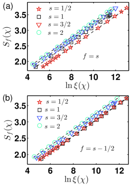
In Fig. 1, we plot the entanglement entropy $S_{f}(\chi)$ versus $\ln\xi(\chi)$ for the spin-$s$ Heisenberg ferromagnetic model (3) with $s=1/2,1,3/2$ and $2$. Here we have chosen different fillings: (a) $f=s$ and (b) $f=s-1/2$, with the bond dimension $\chi$ ranging from $20$ to $160$. To this end, the unit cell in the iMPS representation consists of two lattice sites. For $f=s$, the number of type-B GMs is extracted to be $N_{B}=0.9924,0.9904,0.992$ and $0.9912$ for $s=1/2,1,3/2$ and $2$, respectively. The relative error is less than $1\%$, if we adopt the value of the dynamical critical exponent to be $z=2$, as predicted from the conventional spin wave theory. Conversely, the other way around is to extract the dynamical critical exponent if we adopt $N_{B}=1$. The dynamical critical exponent is extracted to be $z=2.0153,2.0194,2.0161$ and $2.0178$ for $s=1/2,1,3/2$ and $2$, respectively. The relative error is less than $1\%$. Similarly, for $f=s-1/2$, the number of type-B GMs is extracted to be $N_{B}=0.9928,0.992,0.9904$ and $0.9916$ for $s=1/2,1,3/2$ and $2$, respectively. Then a relative error is less than $1\%$, if we adopt the dynamical critical exponent value $z=2$. Conversely, the dynamical critical exponent is extracted to be $z=2.0145,2.0161,2.0194$ and $2.0169$ for $s=1/2,1,3/2$ and $2$, respectively, with the relative error again less than $1\%$.

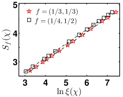
In Fig. 2, we plot the entanglement entropy $S_{f}(\chi)$ versus $\ln\xi(\chi)$ for the $\rm{SU}(3)$ ferromagnetic model (4). The filling factors are chosen to be $f=(1/3,1/3)$ and $f=(1/4,1/2)$, with the bond dimension $\chi$ ranging from $80$ to $1000$. Here the unit cell in the iMPS representation consists of three and four lattice sites, respectively. The number of type-B GMs is extracted to be $N_{B}=1.9804$ for $f=(1/3,1/3)$ and $1.9816$ for $(1/4,1/2)$, with the relative error being less than $1\%$, if we adopt the dynamical critical exponent $z=2$, as predicted from the conventional spin wave theory. Conversely, adopting the value $N_{B}=2$, the dynamical critical exponent is extracted to be $z=2.0198$ for $f=(1/3,1/3)$ and $2.0186$ for $(1/4,1/2)$, with again the relative error less than $1\%$.

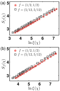
Fig. 3 shows plots of the entanglement entropy $S_{f}(\chi)$ versus $\ln\xi(\chi)$ for the ${\rm SO}(4)$ spin-orbital model (5), with (a) $\zeta=3/4$ and (b) $\zeta=\infty$. Here we have chosen the fillings $f=(1/2,1/2)$ and $f=(5/12,5/12)$, with the bond dimension $\chi$ ranging from $100$ to $1000$. The unit cell in the iMPS representation consists of four and six lattice sites, respectively. If we adopt the dynamical critical exponent $z=2$, as predicted from the conventional spin wave theory, the best linear fit is exploited to estimate the number of type-B GMs as $N_{B}=1.9296$ and $1.9468$ in Fig. 3(a), with relative error less than $4\%$, and $N_{B}=1.9512$ and $1.9524$ in Fig. 3(b), with relative error less than $3\%$. Here if we adopt $N_{B}=2$, the dynamical critical exponent is extracted to be $z=2.073$ and $2.059$ in Fig. 3(a) and $z=2.05$ and $2.0488$ in Fig. 3(b), with in each case a relative error less than $4\%$.

A generic scheme to perform a finite-entanglement scaling analysis has been put forward for highly degenerate ground states arising from SSB with type-B GMs, which are scale-invariant, but not conformally invariant. Extensive numerical simulations have been performed for the three selected models – the spin-$s$ Heisenberg ferromagnetic model, the $\rm{SU}(3)$ ferromagnetic model and the $\rm{SO}(4)$ spin-orbital model. Actually, the number of type-B GMs $N_{B}$ may be reliably extracted from finite block-size scaling, as long as the bond dimension $\chi$ is large enough, within a reasonable accuracy. A detailed exposition for a finite block-size scaling analysis to extract the number of type-B GMs has been described in Section D of the SM. This in turn allows us to extract the dynamical critical exponent from finite-entanglement scaling.