Fair Regression for Health Care Spending
Abstract
The distribution of health care payments to insurance plans has substantial consequences for social policy. Risk adjustment formulas predict spending in health insurance markets in order to provide fair benefits and health care coverage for all enrollees, regardless of their health status. Unfortunately, current risk adjustment formulas are known to underpredict spending for specific groups of enrollees leading to undercompensated payments to health insurers. This incentivizes insurers to design their plans such that individuals in undercompensated groups will be less likely to enroll, impacting access to health care for these groups. To improve risk adjustment formulas for undercompensated groups, we expand on concepts from the statistics, computer science, and health economics literature to develop new fair regression methods for continuous outcomes by building fairness considerations directly into the objective function. We additionally propose a novel measure of fairness while asserting that a suite of metrics is necessary in order to evaluate risk adjustment formulas more fully. Our data application using the IBM MarketScan Research Databases and simulation studies demonstrate that these new fair regression methods may lead to massive improvements in group fairness (e.g., 98%) with only small reductions in overall fit (e.g., 4%).
Keywords: Constrained regression, Penalized regression, Risk adjustment, Fairness
1 Introduction
Risk adjustment is a method for correcting payments to health insurers such that they reflect the cost of their enrollees relative to enrollee health. It is implemented by most federally regulated health insurance markets in the United States, including Medicare Advantage and the individual health insurance Marketplaces created by the Affordable Care Act, to prevent losses to insurers who take on sicker enrollees (Pope et al., 2004, McGuire et al., 2013, Kautter et al., 2014). Current risk adjustment formulas use ordinary least squares (OLS) linear regression to predict health plan payments with select demographic information and diagnosis codes from medical claims. These OLS-based formulas are then typically evaluated with overall measures of statistical fit, such as .
While is an important benchmark for evaluating global fit, it lacks information on other dimensions. As a result, risk adjustment has been criticized for not incentivizing efficient payment systems, spending, or population health management (Ash and Ellis, 2012, Layton et al., 2017), and for poorly estimating health costs for some groups by underpredicting their spending relative to average observed spending in the group. Underpredicting spending leads to undercompensation to the insurer, and there is evidence that insurers adjust the prescription drugs, services, and providers they cover (i.e., benefit design) to make health plans less attractive for enrollees in undercompensated groups (Shepard, 2016, Carey, 2017, Geruso et al., 2017). Examples of undercompensated groups include enrollees with specific medical conditions, high-cost enrollees, and partial-year enrollees (van Kleef et al., 2013, Montz et al., 2016, Ericson et al., 2017). Recent research has also shown that health plan insurers have the ability to identify undercompensated groups (Jacobs and Sommers, 2015, Geruso et al., 2017, Rose et al., 2017, Withagen-Koster et al., 2018).
What constitutes a fair or unfair algorithm depends heavily on the context. These fairness concepts and methods have been largely developed in the computer science literature (Chouldechova and Roth, 2018). We will consider risk adjustment formulas unfair if they underpredict spending for a prespecified group of enrollees, which then incentivizes differential treatment for the group via benefit design due to this undercompensation. For example, if average observed spending for individuals with mental health and substance use disorders (MHSUD) is 10,000, but average predicted spending in this group is 8,000, the risk adjustment formula may be unfair for the MHSUD group by ‘substantially’ underpredicting their spending. We define formal metrics for evaluating fairness in risk adjustment formulas using group residual errors in the next section.
Methods for addressing fairness are often separated into three categories based on the point in the learning process at which fairness is addressed: the preprocessing, fitting, or postprocessing phase. If the data are inherently biased, then preprocessing techniques are a possible solution. These methods create fair datasets by transforming or changing the data so that it is no longer biased (Kamiran and Calders, 2009, Zliobaite et al., 2011, Zemel et al., 2013, Calmon et al., 2017, Johndrow and Lum, 2017). It has been shown that current spending patterns among various group may be undesirable due to the plan benefit system, and by using observed spending data, we reinforce these unfair spending patterns. A recent study explored this concept by transferring funds to undercompensated groups in the raw data in order to promote more ideal spending patterns (Bergquist et al., 2019).
One of the most common fitting phase approaches in risk adjustment attempts to fix group undercompensation by adding new variables representative of the groups in the risk adjustment formula (van Kleef et al., 2013). While this is a straightforward idea, it can be problematic if those variables are unavailable, incentivize over- or underutilization of health services, or the risk adjustment formula does not recognize the improvement (Rose and McGuire, 2019). Fitting techniques in fairness include separate formulas for protected classes as well as fairness penalty terms or constraints (Kamishima et al., 2012, Berk et al., 2017a, Zafar et al., 2017a, b, Bechavod and Ligett, 2018, Dwork et al., 2018). We see intersections of these areas in the risk adjustment literature with separate formulas for enrollees with MHSUD (Shrestha et al., 2018, van Kleef et al., 2018) and constrained regression to reduce undercompensation for specific groups (van Kleef et al., 2017). Notably, separate risk adjustment formulas are already used in practice for infants and adults due to known differences in spending patterns. Nonparametric statistical machine learning methods to enhance estimation accuracy in risk adjustment have also been explored for the fitting stage (Rose, 2016, Shrestha et al., 2018, Park and Basu, 2018), but none of these tools are currently deployed in the U.S. health care system.
Postprocessing techniques modify the results after fitting by, for example, creating specific classification thresholds for different groups (Bansal et al., 2014, Hardt et al., 2016, Kleinberg et al., 2018, El Mhamdi et al., 2018). These methods separate fit from fairness objectives and allow use of the same prediction function for multiple fairness objectives. Reinsurance, paying insurers for a portion of the costs of high-cost enrollees, can be considered postprocessing for risk adjustment in that it reduces undercompensation for high-risk enrollees (McGuire and van Kleef, 2018).
In this paper, we focus on the fitting phase and expand on concepts from statistics, computer science, and health economics, proposing new estimation methods and measures to improve risk adjustment formulas for undercompensated groups. We develop two new fair regression estimators for continuous outcomes that reduce residual errors for an undercompensated group by building fairness considerations directly into the objective function. We also extend a definition of fairness from the computer science and statistics literature for the risk adjustment setting while additionally considering existing measures.
Our application features the IBM MarketScan Research Databases. This set of databases contains enrollee-level claims, demographic information, and health plan spending for a sample of individuals (and their dependents) insured by private health plans and large employers across the country. In 2014, the IBM MarketScan Research Databases were used by the federal government to develop the risk adjustment formula for the individual health insurance Marketplaces. Thus, this data source is particularly policy relevant. The undercompensated group we focus on for this data application is enrollees with MHSUD. We select this group for two major reasons. First, individuals with MHSUD are known to have substantially undercompensated payments in current risk adjustment formulas (Montz et al., 2016). Second, about 20% of people in the United States have MHSUD, thus it is a priority area for policy change. Although the data are representative of only a subset of the U.S. health insurance market, our methods are appropriate for other markets and different application settings with continuous outcomes. The methods and metrics we present are compared in this data analysis as well as simulation studies.
2 Statistical Framework
This section describes our approach to fair regression. It involves a suite of fairness measures for evaluating new and existing regression tools in an effort to improve risk adjustment formulas for undercompensated groups. A typical algorithmic fairness problem has an outcome and input vector that includes a protected group . The goal is to create an estimator for the function that maps to , while aiming to ensure that the function is fair for protected group . Although our main goal is to understand whether estimation methods beyond OLS, including those we newly propose, improve fairness for risk adjustment, we also wish to focus on interpretability for stakeholders, such as government agencies, insurers, providers, and enrollees. Therefore, constrained and penalized regressions were natural choices to enforce fairness in risk adjustment for undercompensated groups.
2.1 Measures
The most commonly used measures of fairness are based on the notion of group fairness, striving for similarity in predicted outcomes or errors for groups. Let be the set containing all enrollees with MHSUD (i.e., the undercompensated group), indexed by . The complement group, all enrollees without MHSUD, is denoted by and indexed by . Overall sample size, , is indexed by . Group undercompensation is a result of large average group residuals in the risk adjustment formula. We define fairness as a function of these residual errors given that many undercompensated groups have substantially higher average health care costs. Thus, enforcing similar predicted outcomes between and would be unfair to both. In this subsection, we present three relevant existing measures of group fairness, a new extension of fair covariance modified for group fairness with continuous outcomes, and as a metric of overall global fit.
Mean Residual Difference. Comparing mean residual errors between a group and its complement aims to assess fairness by evaluating whether this difference is close to zero (Calders et al., 2013): To date, this metric has not been applied in risk adjustment.
Net Compensation. Net compensation is a related measure from the health economics literature on the same scale as the mean residual difference (Layton et al., 2017). However, it does not contain a term for the mean residual in the complement group: Therefore, this measure focuses on a reduction in the residuals for rather than similarity in residuals between the groups. A parallel net compensation measure can be calculated for .
We highlight that we intentionally take the difference rather than so that undercompensation for those in aligns with a negative value of net compensation, in line with previous literature (e.g., Bergquist et al., 2019). This is reflected in the mean residual difference definition above as well. We do not maintain this ordering for the corresponding estimators in Section 2.2 as we wish to penalize large undercompensation in net compensation penalized regression by adding to the squared error and the squared term for mean residual difference penalized regression negates the ordering distinction.
Predictive Ratios. Predictive ratios are commonly used to quantify the underpayment for specific groups in risk adjustment (Pope et al., 2004): Whereas net compensation provides the absolute magnitude of the loss in dollars, predictive ratios provide the relative size of the loss. Predictive ratios can also be created for .
Fair Covariance. Other fairness work creates a measure based on the idea that to be fair, the predicted outcome (or residual error) and protected class must be independent. Using the covariance between the predicted outcome (or residual error) and the protected class as a proxy for independence, that work establishes a fairness measure (Zafar et al., 2017a, b). Because this prior metric assumes outcomes are classified into discrete categories, we extend the definition to define a new measure of fair covariance for residual errors with continuous . Our measure is given by: , where is the random variable indicating membership in . This measure is bounded by the covariance of the undercompensated group and the OLS residual, which we refer to as . Our fair covariance measure allows one to see the empirical signal for systematic undercompensation through residual covariance and it can also be scaled by such that it is bounded between 0 and 1.
Global Fit. In addition to fairness measures, we also evaluate overall fit with the traditional measure used in risk adjustment, which is : , where we recall that indexes the overall sample. Given current policymaker prioritization of global metrics, it is important to compare estimators with both group and overall fit measures to understand the impact on global fit when seeking fairness for undercompensated groups.
The measures we consider above assume that the data include unbiased , which may not be the case in practice. Additionally, fairness is frequently assessed for one or two groups, as we also do here. In reality, we are often concerned about fairness for many groups. This requires the ability to define all meaningful groups, which is not always an objective task. There are also tradeoffs involved in selecting a fairness metric, and ensuring fairness based on one definition does not necessarily guarantee a satisfying solution with respect to other fairness measures or overall fit (Kleinberg et al., 2016, Chouldechova, 2017, Berk et al., 2017b). We return to these issues in our discussion. In Web Appendix A, we present a new extension of a fairness measure for comparing individual residual errors rather than mean residual errors. This Group Residual Difference metric is not practical to implement at scale in risk adjustment, thus we do not deploy it here, but could be useful for settings where is smaller.
2.2 Estimation Methods
We present five methods that incorporate a fairness objective with a constraint or penalty to improve risk adjustment formulas for undercompensated groups. Two of these methods, covariance constrained regression and net compensation penalized regression, are new contributions, and all five methods will also be compared to the OLS estimator. We have a continuous spending outcome , a vector of binary health variables , an input vector , and a coefficient vector indexed by . For OLS, we aim to solve the following regression problem:
| (1) |
Average Constrained Regression. A previously proposed constrained regression method for risk adjustment requires that the estimated average spending for the undercompensated group is equal to the average spending, which means that net compensation for the undercompensated group is zero (van Kleef et al., 2017). This is achieved by including a constraint: , subject to The given constraint has been applied in the risk adjustment literature to reduce undercompensation for select groups (van Kleef et al., 2017, Bergquist et al., 2019).
Weighted Average Constrained Regression. The next existing method relaxes the previous constraint, allowing the estimated spending to be a weighted average of the average spending of the undercompensated group and the estimated spending under unconstrained OLS: , subject to where is the coefficient vector from the OLS given in formula (1). The hyperparameter is a weighting factor. When , this method is equivalent to average constrained regression, and when it is equivalent to OLS. Weighted average constrained regression has been shown to reduce undercompensation for select groups in the Netherlands risk adjustment formula (van Kleef et al., 2017).
Covariance Constrained Regression. The class of covariance methods we consider impose a constraint on the residual by requiring that the covariance between the residual and the protected class is close to zero (Zafar et al., 2017a, b). We extend these techniques to propose a new method for our risk adjustment setting where we have a continuous residual, which has not been previously explored. In order to solve the optimization problem, we convert it into a convex problem. We simplify the covariance as follows:
Now that we have the covariance in the form of a convex problem, we can define what we need to solve: , subject to and . Parallel to the literature for discrete categories (Zafar et al., 2017b), we set , where is a multiplicative factor and is the covariance of the undercompensated group and the OLS residual. The upper bound for occurs at , which is .
As we are primarily concerned with the residual of the undercompensated group being too large, we choose to instead bound the covariance on one side in our implementation of this method. In other words, we constrain the covariance to be less than some percentage of the OLS covariance (as defined by the hyperparameter ). A one-sided constraint also yields faster optimization. The updated optimization problem is: , subject to .
Mean Residual Difference Penalized Regression. The relationship between penalized and constrained regressions is well recognized in statistics (Hastie et al., 2009), and one could equivalently reformulate the above constraints as penalties. Penalized regression has also been explored in the fairness literature. Calders et al. (2013) consider constrained formulations of their approaches, but propose the flexibility of penalization as an alternative due to the possibility of degenerate solutions with a high number of constraints. In their mean residual difference regression technique, one penalizes with large mean residual differences between the undercompensated group and the complement group. The coefficients minimize: , where hyperparameter can be user-specified or chosen via cross-validation, and its magnitude will be on the same scale as .
Net Compensation Penalized Regression. In our second new method, rather than imposing a constraint, we also formulate a penalized regression. Our regression involves the inclusion of a custom net compensation penalty term in the minimization problem: . This penalty punishes estimators where the net compensation, or difference between the average spending and predicted spending for the undercompensated group, is large. We can alternatively present our new method as a constraint: , subject to , where the hyperparameter is positive and has a one-to-one correspondence with, but is not equal to, when the constraint is binding. We choose to primarily implement this method as a penalized regression to explore differences in performance with the mean residual difference penalized regression for the same values of . However, simulation studies in Web Appendix B of the Supplementary Material examine the performance of the constrained formulation.
2.3 Computational Implementation
These six methods were evaluated to assess both overall fit and fairness goals with 5-fold cross-validation in our data analysis and simulations using the suite of five measures defined in Section 2.1. OLS was implemented in the R programming language with the lm() function. All other estimators were optimized using the CVXR package. This package uses disciplined convex programming to solve optimization problems and allows users to specify novel constraints and penalties (Fu et al., 2018).
3 Health Care Spending Application
We selected a random sample of 100,000 enrollees from the IBM MarketScan Research Databases. Age, sex, and diagnosed health conditions, all from the year 2015, were used to predict total annual expenditures in 2016. Diagnosed health conditions took the form of the established Hierarchical Condition Category (HCC) variables created for risk adjustment. HCCs were developed by the Department of Health and Human Services to group a selection of International Classification of Disease and Related Health Problems (ICD) codes into indicators for various health conditions (Pope et al., 2004, Kautter et al., 2014). We considered the 79 HCC variables currently used in Medicare Advantage risk adjustment formulas and retained the 62 HCCs that had at least 30 enrollees with the condition. See Web Appendix C for a list of the 62 HCCs included in the regression formulas. Our sample of enrollees was 52% female and between the ages of 21 and 63, with median age 45. Mean and median annual expenditures per enrollee were $6,651 and $1,511, respectively.
We defined enrollees with MHSUD, our protected group , using Clinical Classification Software (CCS) categories. This classification system maps each MHSUD-related ICD code to a CCS category, unlike the HCCs, which only map a subset of MHSUD-related ICD codes. Based on CCS categories, 13.8% of the sample had a diagnosis code for MHSUD compared to 2.6% had we used HCCs. We note that we do not capture enrollees with MHSUD who do not have an ICD code for their condition(s). The mean annual expenditures for MHSUD enrollees in our sample were $11,520 versus $5,880 for enrollees without MHSUD (and $3,744 versus $1,274 for median annual expeditures).
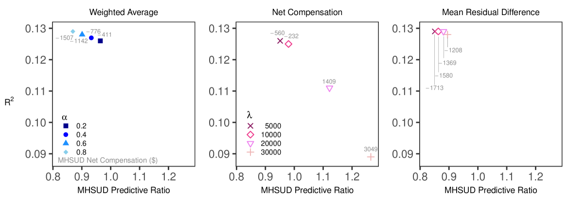
We compared each method to determine which estimators were best at reducing undercompensation for enrollees with MHSUD, and at what cost to overall statistical fit. In Table 1, we report the top estimators with respect to fairness for each of the six methods, having selected the hyperparameter value that optimizes the fairness measures (for those that have these parameters). Hyperparameter values were user-specified from the range of plausible values. For example, in the covariance constrained regression, can range from 0 to 1, and we considered . Comparisons of global fit versus group fairness for the three methods with variation in performance by hyperparameter can be found in Figure 1.
| Predictive | Net | Mean | |||||
|---|---|---|---|---|---|---|---|
| Ratio | Compensation | Residual | Fair | ||||
| Method | Difference | Covariance | |||||
| Average | 12.4% | 0.996 | 1.001 | -$46 | $4 | -$50 | 6 |
| Covariance | 12.4 | 0.996 | 1.001 | -46 | 4 | -50 | 6 |
| Net Compensation† | 12.5 | 0.980 | 1.006 | -232 | 34 | -266 | 31 |
| Weighted Average∓ | 12.6 | 0.964 | 1.011 | -411 | 62 | -473 | 56 |
| Mean Residual Difference⊕ | 12.8 | 0.895 | 1.032 | -1208 | 188 | -1396 | 164 |
| OLS | 12.9 | 0.837 | 1.050 | -1872 | 293 | -2165 | 256 |
, ,
Note: Measures calculated based on cross-validated predicted values and sorted on net compensation. Best performing hyperparameters for each estimator (with respect to fairness measures) are displayed. Performance for covariance method was the same for all . is the complement of g.
OLS had a cross-validated measure of 12.9%, a predictive ratio of 0.837 for individuals with MHSUD, and underestimated average MHSUD spending by -$1,872, with a mean residual difference of -$2,165. The fair covariance measure was 256. Average spending for enrollees without MHSUD was overestimated by $293 with a predictive ratio of 1.050. OLS had the worst performance along all fairness metrics while producing an only trivially higher than the competing methods.
We found the best improvement in fairness for MHSUD using the existing average constrained regression and our new covariance constrained regression. These two methods had similar, although not identical performance, and reduced the average undercompensation for enrollees with MHSUD to -$46 (versus -$1,872 in the OLS), a relative improvement of 98%. They also increased the predictive ratio from 0.837 to 0.996. Enrollees without MHSUD were overestimated by only $4 and had a predictive ratio of 1.001. Both methods reduced the fair covariance measure from 256 to 6. Unsurprisingly, these two estimators were also the worst performers on overall fit as measured by , although it was a loss of only 4%, from 12.9% to 12.4%. This small 0.5 percentage point loss in may be tolerable to policymakers.
Recall that the weighted average constrained regression is a compromise estimator between the OLS and average constrained regression. As approached one in the first panel of Figure 1, the metrics more closely resembled the OLS results. As approached zero we saw values closer to the average constrained regression results, although was not only dominated by the average constrained and covariance constrained regressions, but also the net compensation penalized regression with .
The remaining two methods were regressions with customized penalty terms to punish unfair estimates. Our proposed net compensation penalized regression varied substantially by hyperparameter (see second panel in Figure 1), although was the third best performer overall when 10000. Large values yielded extremely poor performance on both overall fit and fairness. At , dropped by 12% to 11.9%, and when increased to , dropped to 9%, a relative reduction of 29%. These two values led to a large overcompensation for enrollees with MHSUD. The covariance was also negative, indicating that the residual value for MHSUD was systematically too high. The mean residual difference penalized regression was less sensitive to hyperparameters compared to the net compensation penalized regression (see third panel in Figure 1). The best performance for mean residual difference penalized regression was at ; it improved on the MHSUD predictive ratio for OLS by 7% (from 0.837 to 0.895) with an loss of less than 1%. However, the best performing net compensation penalized regression had an 81% improvement over the best performing mean residual difference penalized regression when comparing MHSUD net compensation, as well as large improvements in predictive ratios (0.895 versus 0.980) and fair covariance (164 versus 31).
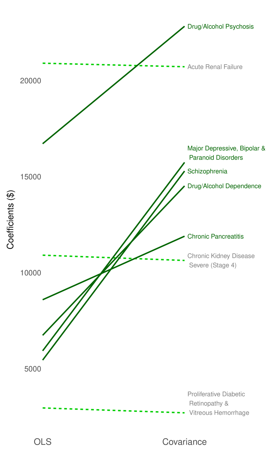
We also examined the HCC variable coefficients for the best performing estimators, the average constrained and covariance constrained regressions, in comparison to OLS. Risk adjustment coefficients communicate incentives to insurers and providers related to prevention and care. For example, coefficients that do not reflect costs can impact an insurer’s incentives in creating their plan offerings. Coefficients for the average constrained and covariance constrained regressions were nearly identical when rounded to the nearest whole dollar, thus we display OLS versus covariance constrained regression in Figure 2. We considered the largest five increases and largest five decreases from OLS to covariance constrained regression, and observed sizable increases in the estimated coefficients associated with MHSUD. The largest relative increase was 180% for “Schizophrenia.” Relative decreases were much smaller.
4 Simulation Study
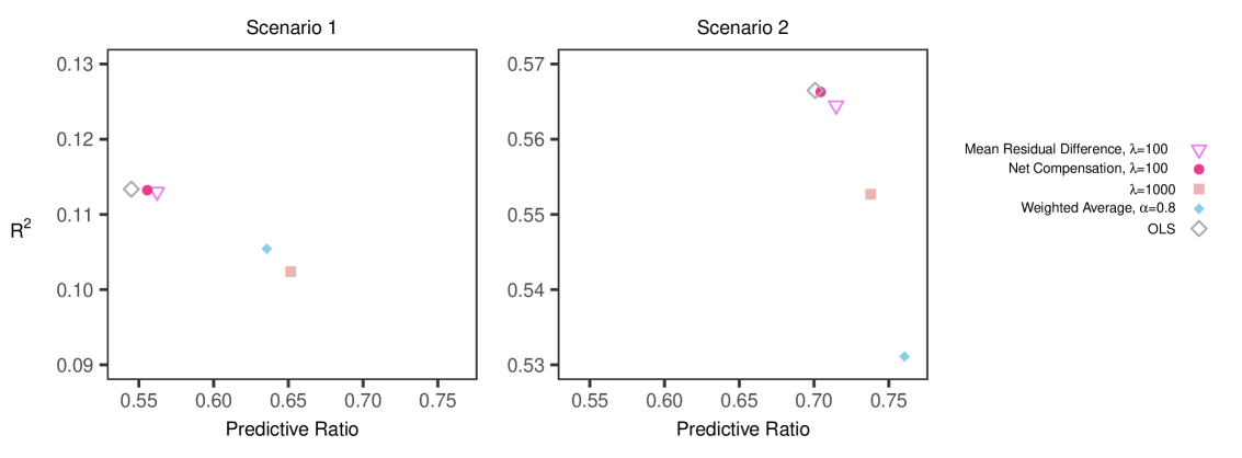
A set of simulation scenarios was developed to explore how these regression methods perform in other settings. We generated a population of 100,000 observations with two continuous outcomes and that were each a function of covariates in and two distinct yet partially overlapping protected classes ( and ) that depended on variables in . Scenario 1 considered a complex functional form for and regression estimators that were misspecified, including omitted variables. Scenario 2 examined a less complex functional form in and regression estimators that were misspecified, including additional noise variables but no omitted variables. A third scenario is discussed in Web Appendix B of the Supplementary Material, along with complete details for the simulated population and first two scenarios. For each scenario, we drew 500 samples of 1,000 and 10,000 observations from the simulated population of 100,000 observations. As in the data analysis, hyperparameter values were user-specified from the range of plausible values.
Selected results are presented in Figure 3, which includes OLS and those methods that improved fairness measures for protected class with a relative loss %. Notably, average constrained and covariance constrained regression, the tied top estimators in our data analysis, do not appear. This was common across settings; average constrained and covariance constrained regression often struggled with functional form misspecification. However, net compensation penalized regression, which performed well in our data analysis, also performed well in the simulations with respect to achieving metric balance between global fit decreases and group fit increases. Additional results are available in Web Appendix B of the Supplementary Material.
5 Discussion
We proposed new fair regression methods aiming to improve risk adjustment for undercompensated groups and asserted that a broader set of metrics is needed. As expected, there was no single method that performed the best across all the measures. One of our newly proposed techniques, net compensation penalized regression, had strong performance with respect to fairness and global fit in both the data analysis and simulations. Selecting the ‘best’ method relies on subjective decisions regarding how to balance group fairness versus overall fit tradeoffs. Improvements in fairness resulted in subsequent decreases in . However, for many estimators, particularly in our data analysis, improvements in fairness were larger than the subsequent decreases in overall fit. This suggests that if we allow for a slight drop in overall fit, we could greatly increase compensation for MHSUD. Policymakers need to consider whether they are willing to sacrifice small reductions in global fit for large improvements in fairness.
We used a sample of enrollees in our demonstration. At scale in a policy implementation, data from millions of enrollees would be used to estimate health spending. Solutions to group undercompensation must be scalable, and current software may or may not yet be capable of handling the sample sizes required. We tested the CVXR optimization package on larger samples and found that it was able to find solutions on a sample of 1,000,000 observations over the span of 3 days (versus 7 hours for the 100,000 enrollee sample). While the optimization results were not within the ideal optimal threshold, they still converged and the results were similar to those presented in this paper, which is promising. Future work includes additional studies regarding scalability. In our analyses, we also considered a selection of user-specified hyperparameter values. A more thorough approach, with possibly improved results, would explore the hyperparameter space in an automated way to select values that optimize over joint fairness and fit objectives. As a general guideline, we found that yielded reasonable metric balance for our newly proposed net compensation penalized regression.
We focused on one group that risk adjustment is known to disadvantage, but it is important to extend such strategies to multiple groups. Improvements for one group could result in subsequent undercompensation for other groups, and balancing fairness across an increasing number of groups is an as yet unsolved problem in risk adjustment. Our simulations examined two protected classes, and we found that improving fairness for one group did not generally help or harm the second group. Earlier research developing methods for the preprocessing phase found that reducing undercompensation for enrollees with MHSUD improved fairness measures for other groups, including enrollees with multiple chronic conditions but without MHSUD. Among the groups included in their comparisons, only enrollees with heart disease had slight reductions in fairness (Bergquist et al., 2019). But even the act of defining the groups poses a problem, as this can be subjective, potentially favoring larger groups with well-funded advocacy organizations. Undercompensation could be undetected in many other lesser-known groups. However, we can only measure undercompensation for groups that are identified by available data, and socioeconomic information, such as poverty and housing, are not available at the individual level for risk adjustment (Ellis et al., 2018).
Broadly, data-driven decisions have come under scrutiny for perpetuating human biases and disparities, which certainly exists in risk adjustment. Arguments for a more comprehensive view of research results is increasing among scientific researchers today (O’Neil, 2017, Gibney, 2018). Recent work argues that evaluating methods from a purely statistical standpoint can lead to negative consequences, and that policy aims should be better incorporated into our research (Corbett-Davies and Goel, 2018). Our article follows in this spirit, and we presented additional estimators and comparisons across multiple measures for the numerous (sometimes competing) goals of risk adjustment. While we worked within the specific context of risk adjustment, the fairness methods and measures discussed here have implications for other settings with continuous outcomes, which have been understudied relative to binary outcomes.
Supplementary Materials
Web Appendix A presents the Group Residual Difference, a new extension of a fairness measure for comparing individual residual errors that is not currently practical to implement at scale in risk adjustment. Web Appendix B, referenced in Sections 2 and 4, describes the simulation study details and results. Web Appendix C is a list of HCCs included in the data analysis regression formulas from Section 3. The IBM MarketScan Research Databases used in Section 3 are not available for public dissemination as they contain protected patient information and we were granted access via a restricted data use agreement. Instead, we generated a simulated version of the analysis data that preserves important relationships while protecting the original content, as described in Web Appendix D. We provide this simulated analysis data with code as well as code to reproduce the simulation study from Section 4 with this submission and online: https://github.com/zinka88/Fair-Regression.
Acknowledgments
This work was supported by the National Institutes of Health through an NIH Director’s New Innovator Award DP2-MD012722. The authors thank the Health Policy Data Science Lab, Thomas G. McGuire, Berk Ustun, José Zubizarreta, and the anonymous reviewers for helpful comments.
Web Appendix A: Group Residual Difference
Group Residual Difference. In the fairness literature, one definition for continuous outcomes is that persons with similar should have similar predicted outcomes regardless of their protected class (Berk et al., 2017a). This relies on a user-defined distance function , such as , to ensure that people who are ‘close’ have similar outcomes. We extend this definition for risk adjustment by comparing residuals rather than predicted outcomes for the two groups: We refer to this new measure as the group residual difference. However, this measure is not practical to implement at scale in risk adjustment, which often involves millions of enrollees. The group residual difference requires comparing the residual of every enrollee in the undercompensated group to every other enrollee in the complement group. This scaling issue was also noted in the earlier work our metric extends upon (Berk et al., 2017a). Our group residual difference metric can be useful in settings where is smaller.
Web Appendix B: Simulation Study Details
As described in Section 4 of the main text, our simulation study population of 100,000 observations considered covariates , two protected class indicator variables ( and ), and two continuous outcome variables ( and ). was generated from a Normal distribution with mean 70 and standard deviation 15. Both and had Poisson distributions, with values of 10 and 35, respectively. The last six covariates () were drawn from Bernoulli distributions with probabilities 0.5, 0.1, 0.05, 0.8, 0.03, and 0.2. and were also drawn from Bernoulli distributions, but depended on other generated variables in the population:
They had prevalence rates of and , respectively, with 2.1% overlap. Both outcomes, and , depended on variables in as well as and :
We estimated regressions in three scenarios representing differing types of functional form misspecification:
Complete results for 500 draws from the population with and are given in Web Tables 1 and 2. Simulation data and complete analytic code to reproduce the simulation analyses are available online: https://github.com/zinka88/Fair-Regression.
| Predictive | Net | |||||
|---|---|---|---|---|---|---|
| Ratio | Compensation | Fair | ||||
| Scenario | Method | Covariance | ||||
| 1 | Net Compensation, | -2901.0 | 5.96 | 3231 | -273 | -198.6 |
| Net Compensation, | -106.9 | 1.63 | 408 | -270 | -25.0 | |
| Average | -8.8 | 0.98 | -15 | -270 | 0.9 | |
| Covariance, | -8.8 | 0.98 | -15 | -270 | 0.9 | |
| Mean Residual Difference, | -7.0 | 0.96 | -28 | -270 | 1.7 | |
| Mean Residual Difference, | -2.0 | 0.89 | -70 | -270 | 4.3 | |
| Weighted Average, | -1.9 | 0.89 | -71 | -270 | 4.4 | |
| Net Compensation Constraint, | 0.1 | 0.86 | -92 | -270 | 5.7 | |
| Weighted Average, | 3.5 | 0.80 | -128 | -269 | 7.9 | |
| Weighted Average, | 7.3 | 0.72 | -185 | -269 | 11.4 | |
| Mean Residual Difference, | 8.7 | 0.67 | -215 | -269 | 13.2 | |
| Net Compensation, | 9.1 | 0.65 | -227 | -269 | 14.0 | |
| Weighted Average, | 9.6 | 0.63 | -241 | -269 | 14.9 | |
| Net Compensation Constraint, | 9.6 | 0.62 | -245 | -269 | 15.1 | |
| Net Compensation Constraint, | 10.4 | 0.54 | -298 | -269 | 18.3 | |
| OLS | 10.4 | 0.54 | -298 | -269 | 18.4 | |
| 2 | Net Compensation, | -3436.9 | 2.53 | 217 | 43 | -13.3 |
| Net Compensation, | -85.7 | 1.07 | 9 | 5 | -0.6 | |
| Average | -33.5 | 0.99 | -1 | 3 | 0.1 | |
| Covariance, | -33.4 | 0.99 | -1 | 3 | 0.1 | |
| Mean Residual Difference, | -26.5 | 0.98 | -3 | 3 | 0.2 | |
| Net Compensation Constraint, | -14.3 | 0.96 | -6 | 3 | 0.4 | |
| Mean Residual Difference, | -5.6 | 0.94 | -8 | 2 | 0.5 | |
| Weighted Average, | -1.5 | 0.93 | -10 | 2 | 0.6 | |
| Net Compensation Constraint, | 17.2 | 0.89 | -16 | 1 | 1.0 | |
| Weighted Average, | 23.5 | 0.87 | -18 | 0 | 1.1 | |
| Net Compensation Constraint, | 39.3 | 0.82 | -25 | -1 | 1.5 | |
| Weighted Average, | 41.3 | 0.82 | -26 | -1 | 1.6 | |
| Mean Residual Difference, | 45.9 | 0.80 | -29 | -2 | 1.8 | |
| Weighted Average, | 52.2 | 0.76 | -34 | -3 | 2.1 | |
| Net Compensation, | 54.4 | 0.74 | -37 | -3 | 2.3 | |
| OLS | 56.0 | 0.70 | -43 | -4 | 2.6 | |
| 3 | Net Compensation, | -726.2 | 1.00 | 1 | 44 | 0.0 |
| Average | -582.7 | 0.97 | -5 | 39 | 0.3 | |
| Covariance, | -582.4 | 0.97 | -5 | 39 | 0.3 | |
| Net Compensation Constraint, | -472.3 | 0.94 | -9 | 35 | 0.6 | |
| Mean Residual Difference, | -395.8 | 0.91 | -12 | 32 | 0.8 | |
| Weighted Average, | -358.0 | 0.90 | -14 | 31 | 0.9 | |
| Net Compensation Constraint, | -283.7 | 0.87 | -18 | 27 | 1.1 | |
| Weighted Average, | -183.0 | 0.83 | -24 | 22 | 1.5 | |
| Net Compensation Constraint, | -138.0 | 0.81 | -27 | 19 | 1.6 | |
| Mean Residual Difference, | -121.7 | 0.80 | -28 | 18 | 1.7 | |
| Weighted Average, | -57.7 | 0.77 | -33 | 13 | 2.0 | |
| Net Compensation, | 12.0 | 0.71 | -42 | 6 | 2.6 | |
| Weighted Average, | 18.0 | 0.70 | -43 | 5 | 2.6 | |
| Mean Residual Difference, | 37.5 | 0.66 | -48 | 0 | 2.9 | |
| Net Compensation, | 43.5 | 0.64 | -51 | -3 | 3.1 | |
| OLS | 44.0 | 0.63 | -52 | -4 | 3.2 | |
Note: Measures calculated based on cross-validated predicted values and sorted on net compensation. Estimators with negative values are in shaded text.
| Predictive | Net | |||||
|---|---|---|---|---|---|---|
| Ratio | Compensation | Fair | ||||
| Scenario | Method | Covariance | ||||
| 1 | Net Compensation, | -15.9 | 1.08 | 51 | -271 | -3.1 |
| Average | -8.4 | 1.00 | -1 | -271 | 0.1 | |
| Covariance, | -8.4 | 1.00 | -1 | -271 | 0.1 | |
| Weighted Average, | -1.3 | 0.90 | -60 | -271 | 3.7 | |
| Net Compensation Constraint, | 0.8 | 0.88 | -81 | -271 | 5.0 | |
| Mean Residual Difference, | 2.6 | 0.85 | -101 | -271 | 6.2 | |
| Weighted Average, | 4.2 | 0.82 | -120 | -271 | 7.3 | |
| Weighted Average, | 8.2 | 0.73 | -179 | -271 | 10.9 | |
| Mean Residual Difference, | 9.8 | 0.67 | -213 | -271 | 13.1 | |
| Net Compensation, | 10.2 | 0.65 | -227 | -271 | 13.9 | |
| Weighted Average, | 10.5 | 0.64 | -238 | -271 | 14.6 | |
| Net Compensation Constraint, | 10.6 | 0.63 | -241 | -271 | 14.8 | |
| Mean Residual Difference, | 11.3 | 0.56 | -286 | -271 | 17.5 | |
| Net Compensation, | 11.3 | 0.56 | -290 | -271 | 17.7 | |
| Net Compensation Constraint, | 11.3 | 0.55 | -297 | -271 | 18.2 | |
| OLS | 11.3 | 0.55 | -297 | -271 | 18.2 | |
| 2 | Average | -31.2 | 1.00 | 0 | 3 | 0.0 |
| Covariance, | -31.2 | 1.00 | 0 | 3 | 0.0 | |
| Net Compensation Constraint, | -12.2 | 0.97 | -5 | 3 | 0.3 | |
| Weighted Average, | 0.4 | 0.94 | -9 | 2 | 0.5 | |
| Mean Residual Difference, | 12.3 | 0.91 | -12 | 1 | 0.8 | |
| Net Compensation Constraint, | 18.8 | 0.90 | -15 | 1 | 0.9 | |
| Net Compensation, | 22.6 | 0.89 | -16 | 1 | 1.0 | |
| Weighted Average, | 25.0 | 0.88 | -17 | 0 | 1.1 | |
| Net Compensation Constraint, | 40.6 | 0.83 | -24 | -1 | 1.5 | |
| Weighted Average, | 42.6 | 0.82 | -26 | -1 | 1.6 | |
| Mean Residual Difference, | 47.1 | 0.80 | -29 | -2 | 1.8 | |
| Weighted Average, | 53.1 | 0.76 | -34 | -3 | 2.1 | |
| Net Compensation, | 55.3 | 0.74 | -37 | -3 | 2.3 | |
| Mean Residual Difference, | 56.4 | 0.72 | -41 | -4 | 2.5 | |
| Net Compensation, | 56.6 | 0.71 | -42 | -4 | 2.6 | |
| OLS | 56.6 | 0.70 | -43 | -4 | 2.6 | |
| 3 | Average | -637.6 | 1.00 | -1 | 44 | 0.0 |
| Covariance, | -637.5 | 1.00 | -1 | 44 | 0.0 | |
| Net Compensation Constraint, | -517.1 | 0.96 | -5 | 40 | 0.3 | |
| Weighted Average, | -392.3 | 0.92 | -11 | 34 | 0.7 | |
| Net Compensation Constraint, | -311.2 | 0.89 | -15 | 31 | 0.9 | |
| Weighted Average, | -201.5 | 0.85 | -21 | 25 | 1.3 | |
| Net Compensation Constraint, | -152.2 | 0.83 | -25 | 22 | 1.5 | |
| Weighted Average, | -65.1 | 0.78 | -32 | 15 | 2.0 | |
| Mean Residual Difference, | -28.7 | 0.75 | -36 | 12 | 2.2 | |
| Weighted Average, | 16.7 | 0.70 | -42 | 5 | 2.6 | |
| Net Compensation, | 37.3 | 0.67 | -47 | 1 | 2.9 | |
| Mean Residual Difference, | 38.7 | 0.66 | -48 | 0 | 3.0 | |
| Net Compensation, | 43.8 | 0.64 | -52 | -3 | 3.2 | |
| Mean Residual Difference, | 44.0 | 0.63 | -52 | -4 | 3.2 | |
| Net Compensation, | 44.1 | 0.63 | -53 | -4 | 3.2 | |
| OLS | 44.1 | 0.63 | -53 | -4 | 3.2 | |
Note: Measures calculated based on cross-validated predicted values and sorted on net compensation. Estimators with negative values are in shaded text.
Web Appendix C: Hierarchical Condition Category (HCC) Variables
| HCC | Description |
|---|---|
| 1 | HIV/AIDS |
| 2 | Septicemia, Sepsis, Systemic Inflammatory Response Syndrome/Shock |
| 6 | Opportunistic Infections |
| 8 | Metastatic Cancer and Acute Leukemia |
| 9 | Lung and Other Severe Cancers |
| 10 | Lymphoma and Other Cancers |
| 11 | Colorectal, Bladder, and Other Cancers |
| 12 | Breast, Prostate, and Other Cancers and Tumors |
| 17 | Diabetes with Acute Complications |
| 18 | Diabetes with Chronic Complications |
| 19 | Diabetes without Complication |
| 21 | Protein-Calorie Malnutrition |
| 22 | Morbid Obesity |
| 23 | Other Significant Endocrine and Metabolic Disorders |
| 27 | End-Stage Liver Disease |
| 28 | Cirrhosis of Liver |
| 29 | Chronic Hepatitis |
| 33 | Intestinal Obstruction/Perforation |
| 34 | Chronic Pancreatitis |
| 35 | Inflammatory Bowel Disease |
| 39 | Bone/Joint/Muscle Infections/Necrosis |
| 40 | Rheumatoid Arthritis and Inflammatory Connective Tissue Disease |
| 46 | Severe Hematological Disorders |
| 47 | Disorders of Immunity |
| 48 | Coagulation Defects and Other Specified Hematological Disorders |
| 54 | Drug/Alcohol Psychosis |
| 55 | Drug/Alcohol Dependence |
| 57 | Schizophrenia |
| 58 | Major Depressive, Bipolar, and Paranoid Disorders |
| 72 | Spinal Cord Disorders/Injuries |
| 75 | Myasthenia Gravis/Myoneural Disorders, Inflammatory and Toxic Neuropathy |
| 77 | Multiple Sclerosis |
| 78 | Parkinson’s and Huntington’s Diseases |
| 79 | Seizure Disorders and Convulsions |
| 80 | Coma, Brain Compression/Anoxic Damage |
| 84 | Cardio-Respiratory Failure and Shock |
| 85 | Congestive Heart Failure |
| 86 | Acute Myocardial Infarction |
| 87 | Unstable Angina and Other Acute Ischemic Heart Disease |
| 88 | Angina Pectoris |
| 96 | Specified Heart Arrhythmias |
| 99 | Cerebral Hemorrhage |
| 100 | Ischemic or Unspecified Stroke |
| 103 | Hemiplegia/Hemiparesis |
| 107 | Vascular Disease with Complications |
| 108 | Vascular Disease |
| 111 | Chronic Obstructive Pulmonary Disease |
| 112 | Fibrosis of Lung and Other Chronic Lung Disorders |
| 114 | Aspiration and Specified Bacterial Pneumonias |
| 122 | Proliferative Diabetic Retinopathy and Vitreous Hemorrhage |
| 134 | Dialysis Status |
| 135 | Acute Renal Failure |
| 136 | Chronic Kidney Disease, Stage 5 |
| 137 | Chronic Kidney Disease, Severe (Stage 4) |
| 161 | Chronic Ulcer of Skin, Except Pressure |
| 167 | Major Head Injury |
| 169 | Vertebral Fractures without Spinal Cord Injury |
| 170 | Hip Fracture/Dislocation |
| 173 | Traumatic Amputations and Complications |
| 176 | Complications of Specified Implanted Device or Graft |
| 186 | Major Organ Transplant or Replacement Status |
| 188 | Artificial Openings for Feeding or Elimination |
Web Appendix D: Simulated Analysis Data
The IBM MarketScan Research Databases analyzed in Section 3 of the manuscript cannot be distributed online due to their proprietary nature. They also contain protected patient information. Thus, we created a simulated data set with similar properties using key features and relationships from the original data for reproducibility analyses of our code. The simulated analysis data described below and accompanying code to complete the analyses are available online: https://github.com/zinka88/Fair-Regression.
First, we simulated demographic variables, female and age, by sampling from a Bernoulli distribution, , and truncated Normal distribution with lower bound and upper bound : Next, we generated the 62 binary health variables , each drawn from a Bernoulli distribution and dependent on the demographic variables female and age with coefficients determined by the relationships in the original data. To create the indicator for MHSUD, , we generated 15 binary MHSUD CCS variables dependent on age, female, and the top six HCCs correlated with MHSUD in the original data. We defined for all observations with at least one MHSUD CCS; 15.7% of observations in the simulated analysis data had MHSUD compared to 13.8% in the original data.
To generate , we added random noise to an intermediary outcome dependent on the input vector . We note that while was used to generate , it is not used later in the estimation steps as this information is not currently included in risk adjustment formulas. was determined using a 2-part model. First, to capture the 10.5% of observations without spending in the original data, we generated whether any spending occurred by creating a binary variable with , where and is a vector of coefficients based on the original data. Next, for observations with positive spending, we generated the amount of spending that occurred using a log-linear model of spending dependent on to account for the right-skew of the spending outcome:
where is a vector of coefficients based on the original data. Lastly, we sampled from a truncated normal centered around each observation in to add noise to the generated outcome: where is the predicted outcome for observation in the simulated data. The final simulated spending outcome ranged from $0 to $297,206 with a mean of $5,817 and median of $4,881. The average spending for enrollees with MHSUD was $6,812 versus $5,632 for enrollees without MHSUD. under OLS was 19.7%.
The results from the simulated analysis data are shown in Web Table 3. As demonstrated in our data analysis presented in Section 3 of the main text, we likewise find that the constrained and penalized estimation methods improve fairness measures without a significant decrease in . The relative rankings of all the methods are similar, although we highlight that net compensation penalized regression performs even more similarly to average constrained and covariance constrained regression methods here.
| Predictive | Net | Mean | |||||
|---|---|---|---|---|---|---|---|
| Ratio | Compensation | Residual | Fair | ||||
| Method | Difference | Covariance | |||||
| Net Compensation† | 18.5% | 1.001 | 1.000 | $6 | -$1 | $7 | -1 |
| Average | 18.6 | 0.999 | 1.000 | -5 | 1 | -7 | 1 |
| Covariance | 18.6 | 0.999 | 1.000 | -5 | 1 | -7 | 1 |
| Weighted Average∓ | 19.0 | 0.984 | 1.004 | -106 | 20 | -127 | 17 |
| Mean Residual Difference⊕ | 19.6 | 0.947 | 1.012 | -364 | 68 | -432 | 57 |
| OLS | 19.7 | 0.925 | 1.017 | -512 | 95 | -607 | 80 |
, ,
Note: Measures calculated based on cross-validated predicted values and sorted on net compensation. Best performing hyperparameters for each estimator (with respect to fairness measures) are displayed. Performance for covariance method was the same for all . is the complement of g.
REFERENCES
- Ash and Ellis (2012) Ash, AS. and Ellis, RP. (2012), “Risk-adjusted payment and performance assessment for primary care.” Med Care, 50, 643–653.
- Bansal et al. (2014) Bansal, G., Sinha, A., and Zhao, H. (2014), “Tuning Data Mining Methods for Cost-Sensitive Regression: A Study in Loan Charge-Off Forecasting,” Journal of Management Information Systems, 25, 315–336.
- Bechavod and Ligett (2018) Bechavod, Y. and Ligett, K. (2018), “Penalizing Unfairness in Binary Classification,” arXiv pre-print. arxiv.org/abs/1707.00044.
- Bergquist et al. (2019) Bergquist, SL., Layton, TJ., McGuire, TG., and Rose, S. (2019), “Data transformations to improve the performance of health plan payment methods,” Journal of Health Economics, 66, 195 – 207.
- Berk et al. (2017a) Berk, R., Heidari, H., Jabbari, S., Joseph, M., Kearns, M., Morgenstern, J., Neel, S., and Roth, A. (2017a), “A Convex Framework for Fair Regression,” arXiv pre-print. arxiv.org/abs/1706.02409.
- Berk et al. (2017b) Berk, R., Heidari, H., Jabbari, S., Kearns, M., and Roth, A. (2017b), “Fairness in Criminal Justice Risk Assessments: The State of the Art,” arXiv pre-print. arxiv.org/abs/1703.09207.
- Calders et al. (2013) Calders, T., Karim, A., Kamiran, F., Ali, W., and Zhang, X. (2013), “Controlling Attribute Effect in Linear Regression,” in 2013 IEEE 13th International Conference on Data Mining, Dallas, TX, USA.
- Calmon et al. (2017) Calmon, FP., Wei, D., Ramamurthy, KN., and Varshney, KR. (2017), “Optimized Data Pre-Processing for Discrimination Prevention,” arXiv pre-print. arxiv.org/abs/1704.03354.
- Carey (2017) Carey, C. (2017), “Technological Change and Risk Adjustment: Benefit Design Incentives in Medicare Part D,” American Economic Journal: Economic Policy, 9, 38–73.
- Chouldechova (2017) Chouldechova, A. (2017), “Fair prediction with disparate impact: A study of bias in recidivism prediction instruments,” arXiv pre-print. arxiv.org/abs/1610.07524.
- Chouldechova and Roth (2018) Chouldechova, A. and Roth, A. (2018), “The Frontiers of Fairness in Machine Learning,” arXiv pre-print. arxiv.org/abs/1810.08810.
- Corbett-Davies and Goel (2018) Corbett-Davies, S. and Goel, S. (2018), “The Measure and Mismeasure of Fairness: A Critical Review of Fair Machine Learning,” arXiv pre-print. arxiv.org/abs/1808.00023.
- Dwork et al. (2018) Dwork, C., Immorlica, N., Kalai, AT., and Leiserson, M. (2018), “Decoupled classifiers for fair and efficient machine learning,” Proceedings of Machine Learning Research, 81, 119–133.
- Ellis et al. (2018) Ellis, RP., Martins, B., and Rose, S. (2018), “Risk Adjustment for Health Plan Payment,” in Risk Adjustment, Risk Sharing and Premium Regulation in Health Insurance Markets: Theory and Practice, edited by TG. McGuire, and RC. van Kleef. Amsterdam: Elsevier.
- El Mhamdi et al. (2018) El Mhamdi, EM., Guerraoui, R., Hoang, LN., and Maurer, A. (2018), “Removing Algorithmic Discrimination (With Minimal Individual Error),” arXiv pre-print. arxiv.org/abs/1806.02510.
- Ericson et al. (2017) Ericson, KM., Geissler, K., and Lubin, B. (2017), “The Impact of Partial-Year Enrollment on the Accuracy of Risk Adjustment Systems: A Framework and Evidence,” NBER Working Paper #23765. nber.org/papers/w23765.
- Fu et al. (2018) Fu, A., Narasimhan, B., and Boyd, S. (2018), “CVXR: An R Package for Discplined Convex Optimization,” web.stanford.edu/~boyd/papers/pdf/cvxr_paper.pdf, online; 30 July 2018.
- Geruso et al. (2017) Geruso, M., Layton, TJ., and Prinz, D. (2017), “Screening in Contract Design: Evidence from the ACA Health insurance exchanges,” NBER Working Paper #22832. nber.org/papers/w22832.
- Gibney (2018) Gibney, E. (2018), “The ethics of computer science: this researcher has a controversial proposal,” nature.com/articles/d41586-018-05791-w, online; 9 August 2018.
- Hardt et al. (2016) Hardt, M., Price, E., and Srebro, N. (2016), “Equality of Opportunity in Supervised Learning,” arXiv pre-print. arxiv.org/abs/1610.02413.
- Hastie et al. (2009) Hastie, T., Tibshirani, R., and Friedman, J. (2009), The Elements of Statistical Learning: Data Mining, Inference, and Prediction. 2nd Edition, New York City: Springer.
- Jacobs and Sommers (2015) Jacobs, DB. and Sommers, BD. (2015), “Using Drugs to Discriminate – Adverse Selection in the Insurance Marketplace,” NEJM, 372, 399–402.
- Johndrow and Lum (2017) Johndrow, JE. and Lum, K. (2017), “An algorithm for removing sensitive information: application to race-independent recidivism prediction,” arXiv pre-print. arxiv.org/abs/1703.04957.
- Kamiran and Calders (2009) Kamiran, F. and Calders, T. (2009), “Classifying without Discrimination,” in 2009 2nd International Conference on Computer, Control and Communication, Karachi, Pakistan.
- Kamishima et al. (2012) Kamishima, T., Akaho, S., Asoh, H., and Sakuma, J. (2012), “Fairness-Aware Classifier with Prejudice Remover Regularizer,” in Machine Learning and Knowledge Discovery in Databases, vol. 7524.
- Kautter et al. (2014) Kautter, J., Pope, GC., Ingber, M., Freeman, S., Patterson, L., Cohen, M., and Keenan, P. (2014), “The HHS-HCC Risk Adjustment Model for Individual and Small Group Markets under the Affordable Care Act,” Medicare & Medicaid Research Review, 4, mmrr2014–004–03–a03.
- Kleinberg et al. (2018) Kleinberg, J., Ludwig, J., Mullainathan, S., and Rambachan, A. (2018), “Algorithmic Fairness,” AEA Papers and Proceedings, 108, 22–27.
- Kleinberg et al. (2016) Kleinberg, J., Mullainathan, S., and Raghavan, M. (2016), “Inherent Trade-Offs in the Fair Determination of Risk Scores,” arXiv pre-print. arxiv.org/abs/1609.05807.
- Layton et al. (2017) Layton, TJ., Ellis, RP., McGuire, TG., and van Kleef, RC. (2017), “Measuring efficiency of health plan payment systems in managed competition health insurance markets,” Journal of Health Economics, 56, 237–255.
- McGuire and van Kleef (2018) McGuire, T. and van Kleef, R. (eds.) (2018), Risk Adjustment, Risk Sharing and Premium Regulation in Health Insurance Markets, Amsterdam: Elsevier.
- McGuire et al. (2013) McGuire, TG., Glazer, J., Newhouse, JP., Normand, SL., Shi, J., Sinaiko, AD., and Zuvekas, SH. (2013), “Integrating Risk Adjustment and Enrollee Premiums in Health Plan Payment,” Journal of Health Economics, 32, 1263–1277.
- Montz et al. (2016) Montz, E., Layton, TJ., Busch, AB., Ellis, RP., Rose, S., and McGuire, TG. (2016), “Risk adjustment simulation: Plans may have incentives to distort mental health and substance use coverage,” Health Affairs, 35, 1022–1028.
- O’Neil (2017) O’Neil, C. (2017), Weapons of Math Destruction, New York City: Broadway Books.
- Park and Basu (2018) Park, S. and Basu, A. (2018), “Alternative evaluation metrics for risk adjustment methods,” Health Economics, 27, 984–1010.
- Pope et al. (2004) Pope, GC., Kautter, J., Ellis, RP., et al. (2004), “Risk Adjustment for Medicare Capitation Payments Using the CMS-HCC Model,” Health Care Financing Review, 25, 119–141.
- Rose (2016) Rose, S. (2016), “A Machine Learning Framework for Plan Payment Risk Adjustment,” Health Services Research, 51, 2358–2374.
- Rose et al. (2017) Rose, S., Bergquist, SL., and Layton, TJ. (2017), “Computational health economics for identification of unprofitable health care enrollees,” Biostatistics, 18, 682–694.
- Rose and McGuire (2019) Rose, S. and McGuire, TG. (2019), “Limitations of P-Values and R-squared for Stepwise Regression Building: A Fairness Demonstration in Health Policy Risk Adjustment,” The American Statistician, 73, 152–156.
- Shepard (2016) Shepard, M. (2016), “Hospital Network Competition and Adverse Selection: Evidence from the Massachusetts Health Insurance Exchange,” NBER Working Paper #22600. nber.org/papers/w22600.
- Shrestha et al. (2018) Shrestha, A., Bergquist, SL., Montz, E., and Rose, S. (2018), “Mental Health Risk Adjustment with Clinical Categories and Machine Learning,” Health Services Research, 53, 3189–3206.
- van Kleef et al. (2017) van Kleef, RC., McGuire, TG., van Vliet, R., and van de Ven, W. (2017), “Improving risk equalization with constrained regression,” The European Journal of Health Economics, 18, 1137–1156.
- van Kleef et al. (2013) van Kleef, RC., van Vliet, RC., and Van de Ven, WP. (2013), “Risk equalization in The Netherlands: an empirical evaluation,” Expert Rev Pharmacoecon Outcomes Res, 13, 829–839.
- van Kleef et al. (2018) van Kleef, RC., van Vliet, RC., and van de Ven, WP. (2018), “Health plan payment in the Netherlands,” in Risk Adjustment, Risk Sharing and Premium Regulation in Health Insurance Markets: Theory and Practice, edited by TG. McGuire, and RC. van Kleef. Amsterdam: Elsevier.
- Withagen-Koster et al. (2018) Withagen-Koster, AA., van Kleef, RC., and Eijkenaar, F. (2018), “Examining unpriced risk heterogeneity in the Dutch health insurance market,” The European Journal of Health Economics, 19, 1351–1363.
- Zafar et al. (2017a) Zafar, MB., Valera, I., Rodriguez, MG., and Gummadi, KP. (2017a), “Fairness Beyond Disparate Treatment & Disparate Impact: Learning Classification without Disparate Mistreatment,” arXiv pre-print. arxiv.org/abs/1610.08452.
- Zafar et al. (2017b) — (2017b), “Fairness Constraints: Mechanisms for Fair Classification,” arXiv pre-print. arxiv.org/abs/1507.05259.
- Zemel et al. (2013) Zemel, R., We, Y., Swersky, K., Pitassi, T., and Dwork, C. (2013), “Learning Fair Representations,” in Proceedings of the 30th International Conference on Machine Learning, PMLR, vol. 28, pp. 325–333, Atlanta, Georgia, USA.
- Zliobaite et al. (2011) Zliobaite, I., Kamiran, F., and Calders, T. (2011), “Handling Conditional Discrimination,” in 2011 IEEE 11th International Conference on Data Mining, pp. 992–1001, Vancouver, BC, Canada.