Fast and Accurate Prediction of Antenna Reflection Coefficients in Planar Layered Media Environment via Generalized Scattering Matrix
Abstract
The numerical algorithm for evaluating the reflection coefficient of an antenna in the presence of the planar layered medium is reformulated using the antenna’s generalized scattering matrix (GSM). The interaction between the antenna and the layered medium is modeled through spherical-to-planar vector wave transformations, ensuring no approximations that could compromise computational accuracy. This theoretical framework significantly reduces algebraic complexity, resulting in a marked increase in the speed of antenna performance evaluation. Excluding the one-time preprocessing cost of obtaining the antenna’s GSM in free space, the numerical evaluation speed of this method exceeds that of the commercial software FEKO by several orders of magnitude, while maintaining nearly identical accuracy.
Index Terms:
Layered media, half-space, generalized scattering matrix, spherical vector waves, plane wave spectrum, antenna reflection coefficients.I Introduction
Parameter measurement of planar layered media is a topic of considerable interest, with wide-ranging applications in pavement thickness assessment [1, 2, 3], moisture detection [4, 5, 6], density evaluation [7, 8], underground coal mining [9], and beyond. These applications often involve solving inverse problems—inferring medium properties from the reflection coefficients of antennas. Modern approaches to inverse problems typically rely on optimization algorithms, which iteratively solve the forward problem to approximate the inverse solution. This makes the computational efficiency of the forward solver a critical factor in the overall performance.
The forward modeling of antenna behavior near planar layered media is commonly based on the spatial-domain dyadic Green’s function for layered media (DGLM), expressed via Sommerfeld integrals [10, 11, 12, 13, 14]. This formulation has been adopted in commercial electromagnetic simulation tools, such as Altair FEKO [15], which employ surface integral equations based on discretized antenna geometries to accurately compute reflection coefficients. However, the high computational cost of a single full-wave simulation significantly limits its usability in optimization-based scenarios that require numerous forward evaluations.
To address this limitation, Lambot et al. pioneered a method that models the antenna as an equivalent point source [16], using its far-field radiation to approximate the reflection response from the layered medium—still based on spatial-domain DGLM. Although evaluating spatial-domain DGLM remains challenging due to the presence of infinite-limit Sommerfeld integrals, the point-source approximation significantly reduces the computational burden by requiring evaluation at only a single location. A key limitation, however, is the assumption that the medium is placed in the far field of the antenna. This was later extended in [17], where a multi-point source model was introduced to enable accurate reflection prediction in near-field scenarios. While this approach enhances accuracy, it also increases the number of DGLM evaluations and requires an additional optimization procedure to determine source positions, introducing nontrivial computational overhead.
More recently, Lambot and colleagues proposed a plane-wave spectrum based technique for estimating antenna reflection coefficients [18]. However, their method neglects evanescent wave contributions and multiple reflections between the antenna and the medium, restricting its applicability to scenarios involving weakly scattering antennas.
Motivated by these limitations, this paper presents a novel method for evaluating the electromagnetic behavior of antennas in the presence of planar layered media, with an emphasis on supporting frequency-domain applications that require repeated reflection coefficient evaluations. These might cover most ground-penetrating radar (GPR) operations and electromagnetic material characterization techniques based solely on reflection data [19, 20]. Our approach recharacterizes antenna transmission, reception, and scattering using the generalized scattering matrix (GSM) framework, expressed in terms of discrete spherical vector wave functions (SVWFs), as opposed to continuous plane-wave spectrum expansions. The interaction between the antenna and the layered medium is modeled algebraically by transforming between SVWFs and planar vector wave functions (PVWFs) [21, 22, 23].
Although our method involves a seemingly complex spherical-planar-spherical waveform transformation, the actual computational effort is modest. While the transformation matrix still requires Sommerfeld integrals, the integration limits are very finite—effectively reducing the complexity to that of standard definite integrals. Compared to the spectral-domain method in [18], which involves double integrals, our approach only requires single integrals. Furthermore, the matrix’s inherent symmetry and sparsity significantly improve numerical efficiency.
As this paper further demonstrates, the SVWF-based framework allows for a compact problem size and makes the inclusion of multiple reflections computationally inexpensive. This enables high-fidelity modeling without compromising accuracy for the sake of speed. Ignoring the one-time preprocessing cost of the free-space antenna characterization, our method achieves several orders of magnitude speedup over full-wave simulations in FEKO, while maintaining near-identical accuracy. This substantial advancement in forward problem efficiency could greatly facilitate the adoption of modern computational techniques in inverse problems involving planar layered media.
II Spherical Vector Waves, Planar Vector Waves and Transformations
A core foundation of this paper is the use of PVWFs and SVWFs, which are extensively utilized in [21, 22, 23, 24]. We adopt the time convention and define the PVWF as follows:
| (1) |
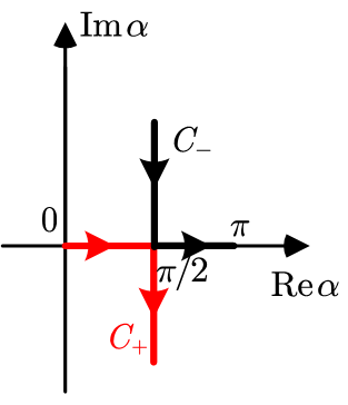
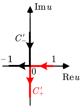
Here, represents the TE wave, and represents the TM wave. The unit vectors are related to the elevation angle and azimuth angle as follows:
| (2) |
The azimuth angle ranges from , while the elevation angle spans . The contours and are illustrated in Fig. 1a. For propagating waves, lies along the real axis between 0 and .
In this paper, we also employ SVWFs , derived from real-valued spherical harmonics [25, Appendix A]. Here, denote regular and outgoing waves, respectively. The subscript indicates polarization type (TE, TM), parity (even, odd), angular degree , and order .
Both SVWFs and PVWFs satisfy the homogeneous vector wave equation, and therefore, they can be converted into one another [24]:
| (3) |
Here, corresponds to , and corresponds to . The integral notation is defined as . The function is given by:
| (4) |
where
Here, the upper (lower) form of applies for even (odd) parity . The is the Kronecker delta. A bar over swaps the TE/TM types of PVWFs (i.e., ). represents the same expression as but with all explicit replaced by . The auxiliary functions
| (5) |
where represents the normalized associated Legendre functions [26]. An efficient algorithm for evaluating these functions for all less than is provided in [26]. This can also be extended to evaluate for imaginary .
A key integral identity used later this work is:
| (6) |
where is nonzero only in the following cases:
III Reflection Coefficient of Antennas in a Layered Planar Environment
The GSM for antennas in free space (the source-scattering formulation) is defined as [27, 28]:
| (7) |
where represents the port S-parameters of the antenna (for a single-mode and single-port antenna, this corresponds to the reflection coefficient), is the receiving matrix, is the transmitting matrix, and is the SVWFs scattering matrix. This paper, building upon previous work [29], uses the method of moments (MoM) to determine the GSM of the antenna.
The GSM relates the incident and response fields of the antenna as:
| (8) |
where and are the expansion coefficients for the incoming and outgoing feeding modes at the antenna ports, respectively. represents the expansion coefficients for the regular spherical wave expansion of the external incident wave , and are the expansion coefficients for the outgoing spherical waves of the antenna’s radiated (scattered) field , specifically:
| (9a) | ||||
| (9b) | ||||
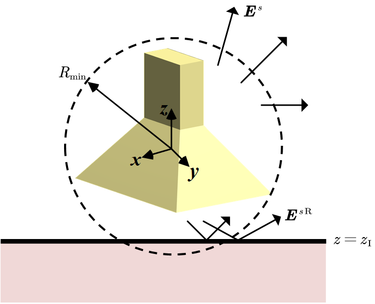
Consider a planar interface located at (with ), as shown in Fig. 2. Further assume that the antenna is actively fed only by wave ports, such that the incident wave entering the antenna from the external space is exclusively the reflected field of , i.e., . To determine , we must calculate how each SVWF component in (9b) is reflected by the interface. To do so, we transform into downward PVWFs using the relation in (3):
| (10) |
The reflected wave of the PVWF , generated by the interface, is given by
| (11) |
where , and is the well-known Fresnel reflection coefficient [see Appendix A]. The phase shift, referenced from the origin, is given by , where . Thus, the reflected wave of can be written as
| (12) |
Equation (3) also provides the SVWF representations for :
| (13) |
where . Consequently, the reflected field can be expressed as
| (14) |
where the -th element of the matrix is given by:
| (15) |
The integral over in (15) can be computed analytically, resulting in the identity in (6). By substituting , we arrive at:
| (16) |
The Sommerfeld integral in (16) traditionally starts from on the contour in Fig. 1b. However, recent research suggests that the starting point of this integral should be truncated by a very finite value , rather than a large value approaching infinite. This modification significantly reduces the computational complexity of (16) while ensuring convergence everywhere above the planar interface. An empirical formula for determining is from [30] as:
| (17) |
which holds for . The maximum degree number is usually chosen as [31]:
| (18) |
where is the minimal radius of the circumscribing sphere around the antenna, and . One can prove the symmetry property , which further reduces the computational burden for evaluating .
With the above results, we can express as
| (19) |
or more compactly:
| (20) |
where
| (21) |
Because GSM connects and as
| (22) |
we substitute into the second equation of (22) to obtain
| (23) |
Solving for gives
| (24) |
where . Substituting this expression into the first equation of (22) leads to the following relation:
| (25) |
This implies that the S-parameters matrix of the antenna near the layered planar medium is
| (26) |
The Neumann series expansion of reads
| (27) |
Each term in this expansion represents interactions of different orders with the layered planar medium. This equation allows for an explicit separation of the contributions from various orders of ground echoes. If multiple reflections between the antenna and the interface are neglected, equation (27) can be approximated by taking only the first term (i.e., the identity matrix ). However, this approximation holds only when the antenna’s scattering is small (). For greater precision, it is usually necessary to consider higher-order terms in the multiple reflections or to directly calculate .
An interesting observation about equation (27) is that are matrices associated with the antenna’s behavior in free space. In contrast, is a matrix that depends on the layered planar medium and the position of the interface , but is independent of the antenna’s characteristics. Therefore, when either or the medium parameters change, only needs to be reevaluated. This process is computationally efficient and can typically be completed within milliseconds, as further detailed in Section IV-D.
IV Numerical Examples
This section demonstrates the numerical performance of the proposed formulas in various planar layered environments. A multi-mode horn antenna, as described in [29], is used as the transmitter. The coordinate origin (geometric center of the antenna) is positioned 80 mm from the radiation aperture. Over the frequency range from 3.2 GHz to 3.8 GHz, the antenna operates in five modes: , , , , and . In the following examples, unless otherwise stated, the maximum degree of SVWFs used is , and the integration truncation number is .
IV-A Example 1—Perfect electric conductor half space
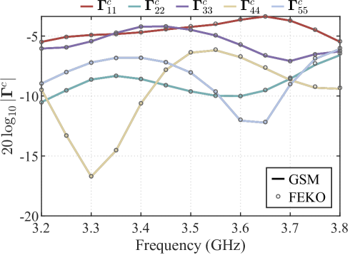
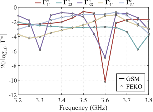
The first example considers a perfect electric conductor (PEC) half-space environment, with the interface located at mm. The distance from the aperture plane to the ground is 120 mm, which is approximately , where represents the low-frequency wavelength. Fig. 3a presents the S-parameters for different modes, with the curve labeled “GSM” representing the results obtained using the method proposed in this paper. A satisfactory agreement is observed when comparing these results with the full-wave simulation results from the FEKO commercial software.
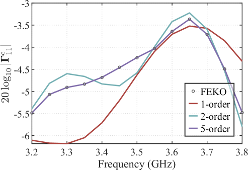
Taking as an example, Fig. 3b illustrates the impact of including different numbers of terms in equation (27) (i.e., accounting for varying orders of ground reflections) on numerical accuracy. It is evident that neglecting multiple reflections (labeled as the “1-order” curve) leads to significant discrepancies when compared with the FEKO results. However, when up to the 5th-order reflections are considered, the results closely match those from FEKO. This highlights the importance of accounting for multiple reflection effects, especially for horn antennas, as traditional methods that neglect multiple reflections may fail to produce accurate results.
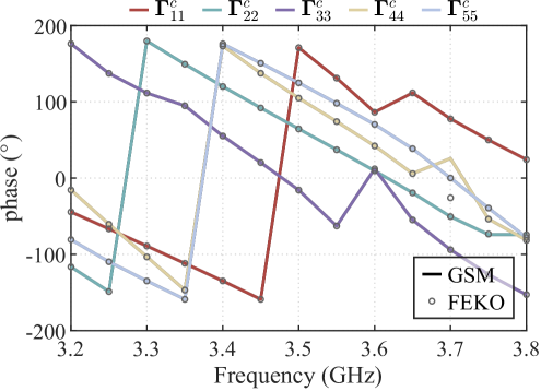
In the next example, we evaluate the numerical accuracy when the antenna is placed very close to the ground. The PEC interface is positioned at mm, where the distance from the horn aperture to the ground is only . To ensure accuracy, we increase the maximum degree of SVWFs to 17 [32], as the sphere circumscribing the horn antenna significantly overlaps with the ground. The truncation number remains at 1.5. Figures 4a and 4b present the magnitude and phase of the antenna’s S-parameters. The results obtained from our method show excellent agreement with those from FEKO, further validating the applicability of our method for accurately predicting antenna performance in near-ground scenarios.
IV-B Example 2—Dielectric material half space
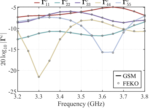
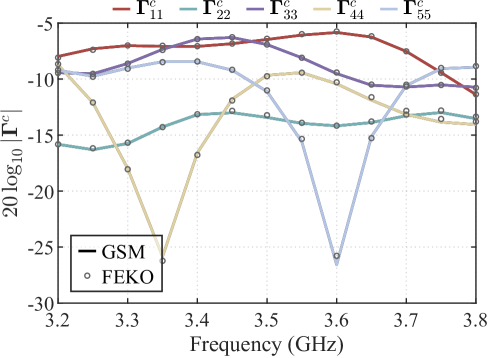
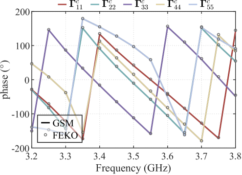
Here, we consider a medium half-space scenario where the material is initially assumed to be seawater (, S/m), with the interface positioned at mm. Figures 5a and 5b present the computed antenna S-parameters. A perfect match is observed when comparing our results with the full-wave simulation data from FEKO.
High-loss scenarios serve as an effective benchmark for evaluating the robustness of most algorithms. To test the capability of our method, we increased the conductivity to S/m and recalculated the antenna’s S-parameters. Figures 6a and 6b show the results, which are in excellent agreement with FEKO, demonstrating that our method can handle high-loss materials effectively.
IV-C Example 3—Layered planar medium environment
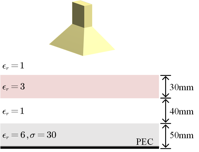
The previous two examples illustrate specific scenarios where our method can be applied. In this final example, we investigate the performance of the same horn antenna in a general multilayer planar medium environment. The FEKO planar multilayer solver (which uses Sommerfeld integrals) supports only simulations with lumped ports, so for this case, the simulation is conducted in free space.
We consider a 5-layer medium structure, as shown in Fig. 7. In the free-space simulation, the lateral dimensions of each layer are set to to model an infinitely large lateral extent. The multilevel fast multipole algorithm (MLFMM) is enabled to run on a 32 GB RAM machine. To ensure the convergence of the MLFMM, the conductivity is kept small. Additionally, smaller permittivities and layer thicknesses are used to reduce the mesh size (with a grid size of ) and ensure the simulation completes within an acceptable time frame. These choices do not affect the generality of the example. The coordinate of the top interface is mm.
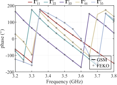
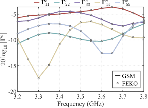
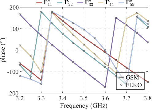
Figures 8a and 8b compare the results from our method with those from the FEKO MLFMM. Both the magnitude and phase of the antenna’s S-parameters show excellent agreement with FEKO results. The minor differences in magnitude at specific frequency points are attributed to the coarse grid discretization and the differences in computational methods.
IV-D Example 4—Demonstration of the implementing time
To implement the proposed method, the GSM of the horn antenna must first be precomputed and stored for each frequency point. In the computational examples presented in the previous subsections, the horn antenna is discretized into 5904 Rao-Wilton-Glisson (RWG) basis functions [33], and the maximum degree of spherical waves is set to . This results in an average computation time of 27 seconds per frequency point when executed on an i5-9400F CPU with 32 GB of RAM.
Next, the transformation matrix needs to be evaluated. In these examples, the calculation of (16) uses a 33-point Gauss-Legendre quadrature rule with a truncation number . The time spent on this procedure per frequency point is approximately 8 ms, and it is almost independent of the layers configurations in the medium.
Finally, the S-parameters are computed using (27), with a computation time of about 7.7 ms. Therefore, excluding the precomputation time for the antenna’s GSM, the total time required to compute the S-parameters is approximately 15.7 ms per frequency point. Notably, since the antenna does not need to be re-simulated when the medium’s material parameters change, new results can be obtained in just 15.7 ms with high accuracy.
As a comparison example, in the half-space case discussed in Sec. IV-B, the FEKO simulation for one frequency point takes approximately 57.6 s using the “reflection coefficient approximation” solver. Furthermore, each time the material parameters change, a new simulation must be run (as the DGLM changes). Although a Sommerfeld integral solver in FEKO cannot be performed with wave port feedings, it would likely take even longer and may fail to converge for thin-layer configurations. These comparisons highlight the significant advantages of the method proposed in this paper.
V Conclusion
This paper introduces a novel numerical method for computing the reflection coefficient of antennas near planar layered media. The method models the transmitting, receiving, and scattering behavior of antennas through a GSM defined by spherical vector wave functions. By expanding SVWFs into PVWFs and applying Fresnel reflection coefficients for the layered medium, the interaction between the antenna and the layered structure is evaluated. Importantly, no approximations are made in this process, ensuring that the computational accuracy matches that of FEKO.
The proposed method benefits from low matrix dimensionality and reduced algebraic complexity. When excluding the one-time preprocessing step to compute the antenna’s GSM in free space, the computation time for each layered media configuration is on the order of milliseconds—vastly outpacing full-wave simulations in FEKO. This makes the method particularly suitable for real-time applications and presents a promising new approach for solving inverse problems involving layered media.
Appendix A Fresnel Reflection Coefficients for Homogeneous Planar Multi-Layers
The reflection coefficient at the - layer interface is given by:
| (28) |
where is the wave impedance of the -th layer medium. Specifically, for TE waves, , and for TM waves, . Here, and , where , , and are the relative permittivity, relative permeability, and conductivity of the -th layer medium, respectively. For a PEC, , while for a perfect magnetic conductor (PMC), .
The longitudinal wavenumber
| (29) |
where is the wavenumber in the -th layer, and is the wavenumber for the top layer (typically free space where the antenna is placed). The convention for the square root is .
With these notations, the Fresnel reflection coefficient at the - layer interface is expressed as:
| (30) |
where denotes the thickness of the -th layer medium. For convenience, the following notations are equivalent: , , and —all representing the Fresnel reflection coefficient of a plane wave incident at the complex elevation angle .
References
- [1] A. Loizos and C. Plati, “Accuracy of ground penetrating radar hornantenna technique for sensing pavement subsurface,” IEEE Sensors J., vol. 7, no. 5, pp. 842-850, May 2007.
- [2] H. Liu and M. Sato, “In situ measurement of pavement thickness and dielectric permittivity by GPR using an antenna array,” NDT & E Int., vol. 64, pp. 65-71, Jun. 2014.
- [3] S. Zhao and I. L. Al-Qadi, “Super-resolution of 3-D GPR signals to estimate thin asphalt overlay thickness using the XCMP method,” IEEE Trans. Geosci. Remote Sens., vol. 57, no. 2, pp. 893-901, Feb. 2019.
- [4] K. Grote, S. Hubbard, J. Harvey, and Y. Rubin, “Evaluation of infiltration in layered pavements using surface GPR reflection techniques,” J. Appl. Geophys., vol. 57, no. 2, pp. 129-153, Feb. 2005.
- [5] J. Minet, P. Bogaert, M. Vanclooster, and S. Lambot, “Validation of ground penetrating radar full-waveform inversion for field scale soil moisture mapping,” J. Hydrol., vol. 424-425, pp. 112-123, Mar. 2012.
- [6] F. M. Fernandes, A. Fernandes, and J. Pais, “Assessment of the density and moisture content of asphalt mixtures of road pavements,” Construct. Building Mater., vol. 154, pp. 1216-1225, Nov. 2017.
- [7] I. L. Al-Qadi, Z. Leng, S. Lahouar, and J. Baek, “In-place hot-mix asphalt density estimation using ground-penetrating radar,” Transp. Res. Rec., J. Transp. Res. Board, vol. 2152, no. 1, pp. 19-27, Jan. 2010.
- [8] S. Zhao, “Development of GPR data analysis algorithms for predicting thin asphalt concrete overlay thickness and density,” Ph.D. dissertation, Dept. Civil Environ. Eng., Univ. Illinois Urbana-Champaign, Champaign, IL, USA, 2018.
- [9] S. B. Thomas and L. P. Roy, “Impact of GPR antenna height in estimating coal layer thickness using spatial smoothing techniques,” IET Sci., Meas. Technol., vol. 14, no. 10, pp. 906-912, Dec. 2020.
- [10] K. A. Michalski and D. Zheng, “Electromagnetic scattering and radiation by surfaces of arbitrary shape in layered media, Part I: Theory,” IEEE Trans. Antennas Propag., vol. 38, pp. 335-344, 1990.
- [11] J. S. Zhao, W. C. Chew, C. C. Lu, E. Michielssen, and J. M. Song, “Thin-stratified medium fast-multipole algorithm for solving microstrip structures,” IEEE Trans. Microwave Theory Tech., vol. 46, no. 4, pp. 395-403, Apr. 1998.
- [12] T. J. Cui and W. C. Chew, “Fast evaluation of sommerfield integrals for em scattering and radiation by three-dimensional buried objects,” IEEE Geosci. Remote Sens., vol. 37, no. 2, pp. 887-900, Mar. 1999.
- [13] W. C. Chew, J. S. Zhao, and T. J. Cui, “The layered medium Green’s function—A new look,” Microwave Opt. Tech. Lett., vol. 31, no. 4, pp. 252-255, 2001.
- [14] W. C. Chew, M. S. Tong, and B. Hu, Integral Equation Methods for Electromagnetic and Elastic Waves. in Synthesis Lectures on Computational Electromagnetics. Cham: Springer International Publishing, 2009. doi: 10.1007/978-3-031-01707-0.
- [15] (2024). Altair FEKO. Altair. [Online]. Available: https://www.altair.com/feko/
- [16] S. Lambot, E. C. Slob, I. van den Bosch, B. Stockbroeckx, and M. Vanclooster, “Modeling of ground-penetrating radar for accurate characterization of subsurface electric properties,” IEEE Trans. Geosci. Remote Sens., vol. 42, no. 11, pp. 2555-2568, Nov. 2004.
- [17] S. Lambot and F. André, “Full-wave modeling of near-field radar data for planar layered media reconstruction,” IEEE Trans. Geosci. Remote Sens., vol. 52, no. 5, pp. 2295-2303, May 2014.
- [18] R. Roohi, A. R. Attari, M. S. Majedi, and S. Lambot, “Prediction of Antenna Reflection Coefficient in Presence of Multilayer Media: A Fast Spectral Domain Approach,” IEEE Trans. Geosci. Remote Sens., vol. 62, 2024.
- [19] S. Liang, C. Shi, and Y. Liu, “A Matrix Pencil-Assisted Parameterized Electromagnetic Parameter Inversion Method for Half-Space Medium via a Single Antenna,” IEEE Trans. Antennas Propagat., vol. 73, no. 2, pp. 1018-1027, Feb. 2025.
- [20] X. Gu, S. Liang, Y. Tang, C. Shi and J. Pan, “Reflection Method for Shielding Effectiveness Measurement: Complex Materials Without Prior Knowledge,” IEEE Trans. Antennas Propag., doi: 10.1109/TAP.2025.3558607.
- [21] G. Kristensson, “Electromagnetic scattering from buried inhomogeneities—a general three-dimensional formalism,” J. Appl. Phys., vol. 51, no. 7, pp. 3486, 1980.
- [22] G. Videen, “Light scattering from a sphere on or near a surface,” J. Opt. Soc. Am. A, vol. 8, no. 3, pp. 483, 1991.
- [23] D. W. Mackowski, “Exact solution for the scattering and absorption properties of sphere clusters on a plane surface,” J. Quant. Spectrosc. Radiat. Transf., vol. 109, no. 5, pp. 770-788, 2008.
- [24] A. Boström, G. Kristensson, and S. Ström, “Transformation properties of plane, spherical and cylindrical scalar and vector wave functions,” in Acoustic, Electromagnetic and Elastic Wave Scattering, Field Representations and Introduction to Scattering, Elsevier, 1991, pp. 165-210.
- [25] V. Losenicky, L. Jelinek, M. Capek, and M. Gustafsson, “Method of Moments and T-Matrix Hybrid,” IEEE Trans. Antennas Propagat., vol. 70, no. 5, pp. 3560-3574, May 2022, doi: 10.1109/TAP.2021.3138265.
- [26] T. Limpanuparb and J. Milthorpe, “Associated Legendre polynomials and spherical harmonics computation for chemistry applications,” arXiv preprint arXiv:1410.1748, 2014.
- [27] J. E. Hansen, Ed., Spherical Near-Field Antenna Measurements. London, U.K.: Peter Peregrinus Ltd., 1988.
- [28] A. D. Yaghjian, Near-field antenna measurements on a cylindrical surface: A source scattering-matrix formulation, Vol. 696, Department of Commerce, National Bureau of Standards, Institute for Basic Standards, Electromagnetics Division, 1977.
- [29] C. Shi, et al., “Generalized Scattering Matrix of Antenna: Moment Solution, Compression Storage and Application,” arXiv preprint arXiv:2411.08904, 2024.
- [30] A. Egel, D. Theobald, Y. Donie, U. Lemmer, and G. Gomard, “Light scattering by oblate particles near planar interfaces: on the validity of the T-matrix approach,” Opt. Express, vol. 24, no. 22, p. 25154, Oct. 2016, doi: 10.1364/OE.24.025154.
- [31] J. Song and W. C. Chew, “Error analysis for the truncation of multipole expansion of vector Green’s functions [EM scattering],” IEEE Microw. Wireless Compon. Lett., vol. 11, no. 7, pp. 311-313, Jul. 2001.
- [32] J. Rubio and R. Gómez-Alcalá, “Mutual coupling of antennas with overlapping minimum spheres based on the transformation between spherical and plane vector waves,” IEEE Trans. Antennas Propag., vol. 69, no. 4, pp. 2103-2111, 2020.
- [33] S. Rao, D. Wilton, and A. Glisson, “Electromagnetic scattering by surfaces of arbitrary shape,” IEEE Trans. Antennas Propagat., vol. 30, no. 3, pp. 409-418, May 1982, doi: 10.1109/TAP.1982.1142818.