Fast and Feature-Complete Differentiable Physics for Articulated Rigid Bodies with Contact

Many modern robotics problems are optimization problems. Finding optimal trajectories, guessing the physical parameters of a world that best fits our observed data, or designing a control policy to optimally respond to a dynamic environment are all types of optimization problems. Optimization methods can be sorted into two buckets: gradient-based, and gradient-free. Despite the well-known drawbacks of gradient-free methods (high sample complexity and noisy solutions), they remain popular in robotics because physics engines with the necessary features to model complex robots are generally non-differentiable. When gradients are required, we typically approximate them using finite differencing [41].

Recent years have seen many differentiable physics engines published [11, 19, 15, 42, 38, 10, 34, 29, 12], but none has yet gained traction as a replacement for popular non-differentiable engines [9, 41, 26]. We hypothesize that an ideal differentiable physics engine needs to implement an equivalent feature set to existing popular non-differentiable engines, as well as provide excellent computational efficiency, in order to gain adoption. In this paper, we extend the existing physics engine DART [26], which is commonly used in robotics and graphics communities, and make it differentiable. Our resulting engine supports all features available to the forward simulation process, meaning existing code and applications will remain compatible while also enjoying new capabilities enabled by efficient analytical differentiability.

A fully-featured physics engine like DART is complex and has many components that must be differentiated. Some components (such as collision detection and contact force computation) are not naively differentiable, but we show that under very reasonable assumptions we can compute useful Jacobians regardless. In order to differentiate through contacts and collision forces, we introduce an efficient method for differentiating the contact Linear Complementarity Problem (LCP) that exploits sparsity, as well as novel contact geometry algorithms and an efficient continuous-time approximation for elastic collisions. As a result, our engine is able to compute gradients with hard contact constraints up to 87 times faster than finite differencing methods, depending on the size of the dynamic system. Our relative speedup over finite differencing grows as the system complexity grows. In deriving our novel method to differentiate through the LCP, we also gain an understanding of the nature of contact dynamics Jacobians that allows us to propose heuristic “complementarity-aware gradients” that may be good search directions to try, if a downstream optimizer is getting stuck in a saddle point.

We provide an open-source implementation of all of these ideas, as well as derivations from previous work [25, 7], in a fully differentiable fork of the DART physics engine, which we call Nimble. Code and documentation are available at nimblephysics.org.

To summarize, our contributions are as follows:

• •

  A novel and fast method for local differentiability of LCPs that exploits the sparsity of the LCP solution, which gives us efficient gradients through static and sliding contacts and friction without changing traditional forward-simulation formulations. Section IV

• •

  A novel method that manipulates gradient computation to help downstream optimization problems escape saddle points due to discrete contact states. Section IV-D

• •

  Fast geometric analytical gradients through collision detection algorithms which support various types of 3D geometry and meshes. Section V

• •

  A novel analytical approximation of continuous-time gradients through elastic contact, which otherwise can lead to errors in discrete-time systems. Section VI

• •

  An open-source implementation of all of our proposed methods (along with analytical gradients through Featherstone first described in GEAR [25]) in a fork of the DART physics engine which we call Nimble. We have created Python bindings and a PyPI package, pip install nimblephysics, for ease of use.

Differentiable physics simulation has been investigated previously in many different fields, including mechanical engineering [16], robotics [14], physics [23, 21] and computer graphics [32, 28]. Enabled by recent advances in automatic differentiation methods and libraries [31, 1, 18], a number of differentiable physics engines have been proposed to solve control and parameter estimation problems for rigid bodies [25, 11, 18, 15, 10, 12, 34] and non-rigid bodies [37, 27, 13, 20, 34, 17, 12]. While they share a similar high-level goal of solving “inverse problems”, the features and functionality provided by these engines vary widely, including the variations in contact handling, state space parameterization and collision geometry support. Table I highlights the differences in a few differentiable physics engines that have demonstrated the ability to simulate articulated rigid bodies with contact. Based on the functionalities each engine intends to support, the approaches to computing gradients can be organized in following categories.

Finite-differencing is a straightforward way to approximate gradients of a function. For a feature-complete physics engine, where analytical gradients are complex to obtain, finite-differencing provides a simpler method. For example, a widely used physics engine, MuJoCo [41], supports gradient computation via finite differencing. However, finite-differencing tends to introduce round-off errors and performs poorly for a large number of input variables.

Automatic differentiation (auto-diff) is a method for computing gradients of a sequence of elementary arithmetic operations or functions automatically. However, the constraint satisfaction problems required by many existing, feature-complete robotic physics engines are not supported by auto-diff libraries. To avoid this issue, many recent differentiable physics engines instead implement impulse-based contact handling, which could lead to numerical instability and constraint violation if the contact parameters are not tuned properly for the specific dynamic system and the simulation task. Degrave et al. [11] implemented a rigid body simulator in the Theano framework [1], while DiffTaichi [18] implemented a number of differentiable physics engines, including rigid bodies, extending the Taichi programming language [19], both representing dynamic equations in Cartesian coordinates and handling contact with impulse-based methods. In contrast, Tiny Differentiable Simulator [15] models contacts as an LCP, but they solve the LCP iteratively via Projected Gauss Siedel (PGS) method [24], instead of directly solving a constraint satisfaction problem, making it possible to compute gradient using auto-diff libraries.

Symbolic differentiation is another way to compute gradients by directly differentiate mathematical expressions. For complex programs like Lagrangian dynamics with constraints formulated as a Differential Algebraic Equations, symbolic differentiation can be exceedingly difficult. Earlier work computed symbolic gradients for smooth dynamic systems [25], and [7] simplified the computation of the derivative of the forward dynamics exploiting the derivative of the inverse dynamics. Symbolic differentiation becomes manageable when the gradients are only required within smooth contact modes [42] or a specific contact mode is assumed [38]. Recently, Amos and Kolter proposed a method, Opt-Net, that back-propagates through the solution of an optimization problem to its input parameters [2]. Building on Opt-Net, de Avila Belbute-Peres et al. [10] derived analytical gradients through LCP formulated as a QP. Their method enables differentiability for rigid body simulation with hard constraints, but their implementation represents 2D rigid bodies in Cartesian coordinates and only supports collisions with a plane, insufficient for simulating complex articulated rigid body systems. More importantly, computing gradients via QP requires solving a number of linear systems which does not take advantage of the sparsity of the LCP structure. Qiao et al. [34] built on [2] and improved the performance of contact handling by breaking a large scene into smaller impact zones. A QP is solved for each impact zone to ensure that the geometry is not interpenetrating, but contact dynamics and conservation laws are not considered. Solving contacts for localized zones has been previously implemented in many existing physics engines [41, 9, 26]. Adapting the collision handling routine in DART, our method by default utilizes the localized contact zones to speed up the performance. Adjoint sensitivity analysis [35] has also been used for computing gradients of dynamics. Millard et al. [29] combined auto-diff with adjoint sensitivity analysis to achieve faster gradient computation for higher-dof systems, but their method did not handle contact and collision. Geilinger et al. [12] analytically computed derivatives through adjoint sensitivity analysis and proposed a differentiable physics engine with implicit forward integration and a customized frictional contact model that is natively differentiable.

Approximating physics with neural networks is a different approach towards differentiable physics engine. Instead of forward simulating a dynamic system from the first principles of Newtonian mechanics, a neural network is learned from training data. Examples of this approach include Battaglia et. al [4], Chang et. al. [8], and Mrowca et. al [30].

Our engine employs symbolic differentiation to compute gradients through every part of the engine using hand-tuned C++ code. We introduce a novel method to differentiate the LCP analytically that takes advantage of the sparsity of the solution and is compatible with using direct methods to solve the LCP. In addition, our engine supports a richer set of geometry for collision and contact handling than has been previously available, including mesh-mesh and mesh-primitive collisions, in order to achieve a fully functional differentiable version of the DART physics engine for robotic applications.

A physics engine can be thought of as a simple function that takes the current position $\boldsymbol{q}_{t}$, velocity $\dot{\boldsymbol{q}}_{t}$, control forces $\boldsymbol{\tau}$ and inertial properties $\boldsymbol{\mu}$, and returns the position and velocity at the next timestep, $\boldsymbol{q}_{t+1}$ and $\dot{\boldsymbol{q}}_{t+1}$:

$$P(\boldsymbol{q}_{t},\dot{\boldsymbol{q}}_{t},\boldsymbol{\tau},\boldsymbol{\mu})=[\boldsymbol{q}_{t+1},\dot{\boldsymbol{q}}_{t+1}].$$

(1)

In an engine with simple explicit time integration, our next position $\boldsymbol{q}_{t+1}$ is a trivial function of current position and velocity, $\boldsymbol{q}_{t+1}=\boldsymbol{q}_{t}+\Delta t\dot{\boldsymbol{q}}_{t}$ , where $\Delta t$ is the descritized time interval.

The computational work of the physics engine comes from solving for our next velocity, $\dot{\boldsymbol{q}}_{t+1}$. We are representing our articulated rigid body system in generalized coordinates using the following Lagrangian dynamic equation:

$$\begin{split}\bm{M}(\bm{q}_{t},\boldsymbol{\mu})\dot{\bm{q}}_{t+1}&=\bm{M}(\bm{q}_{t},\boldsymbol{\mu})\dot{\bm{q}}_{t}-\Delta t(\bm{c}(\bm{q}_{t},\dot{\bm{q}}_{t},\boldsymbol{\mu})-\bm{\tau})\\ &+\bm{J}^{T}(\bm{q}_{t})\bm{f},\end{split}$$

(2)

where $\bm{M}$ is the mass matrix, $\bm{c}$ is the Coriolis and gravitational force, and $\bm{f}$ is the contact impulse transformed into the generalized coordinates by the contact Jacobian matrix $\bm{J}$. Note that multiple contact points and/or other constraint impulses can be trivially added to Equation 2.

Every term in Equation 2 can be evaluated given $\boldsymbol{q}_{t}$, $\dot{\boldsymbol{q}}_{t}$ and $\bm{\tau}$ except for the contact impulse $\boldsymbol{f}$, which requires the engine to form and solve an LCP:

	$\displaystyle\mathrm{find\;\;\;}\bm{f},\bm{v}_{t+1}$
	$\displaystyle\mathrm{such\;that\;\;\;}\bm{f}\geq\bm{0},\;\bm{v}_{t+1}\geq\bm{0},\;\bm{f}^{T}\bm{v}_{t+1}=0.$		(3)

The velocity of a contact point at the next time step, $\bm{v}_{t+1}$, can be expressed as a linear function in $\bm{f}$

	$\displaystyle\bm{v}_{t+1}$	$\displaystyle=\bm{J}\dot{\bm{q}}_{t+1}=\bm{J}\bm{M}^{-1}\left(\bm{M}\dot{\bm{q}}_{t}-\Delta t(\bm{c}-\bm{\tau})+\bm{J}^{T}\bm{f}\right)$
		$\displaystyle=\bm{A}\bm{f}+\bm{b},$		(4)

where $\bm{A}=\bm{J}\bm{M}^{-1}\bm{J}^{T}$ and $\bm{b}=\bm{J}(\dot{\bm{q}}_{t}+\Delta t\bm{M}^{-1}(\bm{\tau}-\bm{c}))$. The LCP procedure can then be expressed as a function that maps $(\bm{A},\bm{b})$ to the contact impulse $\bm{f}$:

$$f_{\text{LCP}}\big{(}\bm{A}(\bm{q}_{t},\boldsymbol{\mu}),\bm{b}(\boldsymbol{q}_{t},\dot{\boldsymbol{q}}_{t},\boldsymbol{\tau},\boldsymbol{\mu})\big{)}=\bm{f}$$

(5)

As such, the process of forward stepping is to find $\bm{f}$ and resulting $\dot{\bm{q}}_{t+1}$ that satisfy Equation 2 and Equation 5.

The main task in developing a differentiable physics engine is to solve for the gradient of next velocity $\dot{\boldsymbol{q}}_{t+1}$ with respect to the input to the current time step, namely $\boldsymbol{q}_{t},\dot{\boldsymbol{q}}_{t},\bm{\tau}_{t}$, and $\bm{\mu}$. The data flow is shown in Figure 2. For brevity we refer to the ouput of a function for a given timestep by the same name as the function with a subscript $t$ (e.g. $\bm{J}_{t}=\bm{J}(\boldsymbol{q}_{t})$). The velocity at the next step can be simplified to

$$\dot{\bm{q}}_{t+1}=\dot{\bm{q}}_{t}+\bm{M}_{t}^{-1}\bm{z}_{t},$$

(6)

where $\boldsymbol{z}_{t}\equiv-\Delta t(\bm{c}_{t}-\bm{\tau}_{t})+\bm{J}_{t}^{T}\bm{f}_{t}$. The gradients we need to compute at each time step are written as:

	$\displaystyle\frac{\partial\dot{\bm{q}}_{t+1}}{\partial\bm{q}_{t}}$	$\displaystyle=\frac{\partial\bm{M}_{t}^{-1}\boldsymbol{z}_{t}}{\partial\boldsymbol{q}_{t}}+\bm{M}_{t}^{-1}\left(-\Delta t\frac{\partial\bm{c}_{t}}{\partial\boldsymbol{q}_{t}}+\frac{\partial\bm{J}_{t}^{T}}{\partial\boldsymbol{q}_{t}}\bm{f}_{t}\right.$
		$\displaystyle\left.+\boldsymbol{J}_{t}^{T}\frac{\partial{\boldsymbol{f}_{t}}}{\partial\boldsymbol{q}_{t}}\right)$		(7)
	$\displaystyle\frac{\partial\dot{\bm{q}}_{t+1}}{\partial\dot{\bm{q}}_{t}}$	$\displaystyle=\bm{I}+\boldsymbol{M}_{t}^{-1}\left(-\Delta t\frac{\partial\boldsymbol{c}_{t}}{\partial\dot{\boldsymbol{q}}_{t}}+\boldsymbol{J}_{t}^{T}\frac{\partial\boldsymbol{f}_{t}}{\partial\dot{\boldsymbol{q}}_{t}}\right)$		(8)
	$\displaystyle\frac{\partial\dot{\bm{q}}_{t+1}}{\partial\bm{\tau}_{t}}$	$\displaystyle=\boldsymbol{M}_{t}^{-1}\left(\Delta t\bm{I}+\boldsymbol{J}_{t}^{T}\frac{\partial\boldsymbol{f}_{t}}{\partial\boldsymbol{\tau}_{t}}\right)$		(9)
	$\displaystyle\frac{\partial\dot{\bm{q}}_{t+1}}{\partial\bm{\mu}}$	$\displaystyle=\frac{\partial\boldsymbol{M}_{t}^{-1}\boldsymbol{z}_{t}}{\partial\boldsymbol{\mu}}+\boldsymbol{M}_{t}^{-1}\left(-\Delta t\frac{\partial\boldsymbol{c}_{t}}{\partial\boldsymbol{\mu}}+\boldsymbol{J}_{t}^{T}\frac{\partial\boldsymbol{f}_{t}}{\partial\boldsymbol{\mu}}\right)$		(10)

We tackle the tricky intermediate Jacobians in sections that follow. In Section IV we will introduce a novel sparse analytical method to compute the gradients of contact force $\boldsymbol{f}_{t}$ with respect to $\boldsymbol{q}_{t},\dot{\boldsymbol{q}}_{t},\bm{\tau}_{t},\bm{\mu}$. Section V will discuss $\frac{\partial\boldsymbol{J}_{t}}{\partial\boldsymbol{q}_{t}}$—how collision geometry changes with respect to changes in position. In Section VI we will tackle $\frac{\partial\boldsymbol{q}_{t+1}}{\partial\boldsymbol{q}_{t}}$ and $\frac{\partial\boldsymbol{q}_{t+1}}{\partial\dot{\boldsymbol{q}}_{t}}$, which is not as simple as it may at first appear, because naively taking gradients through a discrete time physics engine yields problematic results when elastic collisions take place. Additionally, the appendix gives a way to apply the derivations from [25] and [7] to analytically find $\frac{\partial\boldsymbol{M}_{t}^{-1}\boldsymbol{z}_{t}}{\partial\boldsymbol{q}_{t}}$, $\frac{\partial\boldsymbol{c}_{t}}{\partial\boldsymbol{q}_{t}}$, and $\frac{\partial\boldsymbol{c}_{t}}{\partial\dot{\boldsymbol{q}}_{t}}$.

This section introduces a method to analytically compute $\frac{\partial\boldsymbol{f}}{\partial\boldsymbol{A}}$ and $\frac{\partial\boldsymbol{f}}{\partial\boldsymbol{b}}$. It turns out that it is possible to efficiently get unambiguous gradients through an LCP in the vast majority of practical scenarios, without recasting it as a QP (which throws away sparsity information by replacing the complementarity constraint with an objective function). To see this, let us consider a hypothetical LCP problem parameterized by $\boldsymbol{A},\boldsymbol{b}$ with a solution $\boldsymbol{f}^{*}$ found during the forward pass: $f_{\text{LCP}}(\bm{A},\bm{b})=\bm{f}^{*}$.

For brevity, we only include the discussion on normal contact impulses in this section and leave the extension to friction impulses in Appendix -A. Therefore, each element in $\boldsymbol{f}^{*}\geq\boldsymbol{0}$ indicates the normal impulse of a point contact. By complementarity, we know that if some element $f^{*}_{i}>0$, then $v_{i}=(\boldsymbol{A}\boldsymbol{f}^{*}+\boldsymbol{b})_{i}=0$. Intuitively, the relative velocity at contact point $i$ must be 0 if there is any non-zero impulse being exerted at contact point $i$. We call such contact points “Clamping” because the impulse $f_{i}>0$ is adjusted to keep the relative velocity $v_{i}=0$. Let the set $\mathcal{C}$ to be all indices that are clamping. Symmetrically, if $f_{j}=0$, then the relative velocity $v_{j}=(\boldsymbol{A}\boldsymbol{f}^{*}+\boldsymbol{b})_{j}\geq 0$ is free to vary without the LCP needing to adjust $f_{j}$ to compensate. We call such contact points “Separating” and define the set $\mathcal{S}$ to be all indices that are separating. Let us call indices $j$ where $f_{j}=0$ and $v_{j}=0$ “Tied.” Define the set $\mathcal{T}$ to be all indices that are tied.

If no contact points are tied ($\mathcal{T}=\emptyset$), the LCP is strictly differentiable and the gradients can be analytically computed. When some contact points are tied ($\mathcal{T}\neq\emptyset$), the LCP has valid subgradients and it is possible to follow any in an optimization. The tied case is analogous to the non-differentiable points in a QP where an inequality constraint is active while the corresponding dual variable is also zero. In such a case, computing gradients via taking differentials of the KKT conditions will result in a low-rank linear system and thus non-unique gradients [2].

This section addresses efficient computation of $\frac{\partial\boldsymbol{J}_{t}^{T}\boldsymbol{f}}{\partial\boldsymbol{q}_{t}}$, the relationship between position and joint impulse. In theory, we could utilize auto-diff libraries for the derivative computation. However, using auto-diff and passing every gradient through a long kinematic chain of transformations is inefficient for complex articulated rigid body systems. In contrast, computing the gradients symbolically shortcuts much computation by operating directly in the world coordinate frame.

Let $\mathcal{A}_{i}\in se(3)$ be the screw axis for the $i$’th DOF, expressed in the world frame. Let the $k$’th contact point give an impulse $\mathcal{F}_{k}\in dse(3)$, also expressed in the world frame. Let $\psi_{i,k}\in\{-1,0,1\}$ be the relationship between contact $k$ and joint $i$. $\psi_{i,k}=1$ or $\psi_{i,k}=-1$ means contact $k$ is on a child body of joint $i$. Otherwise, $\psi_{i,k}=0$. The total joint impulse caused by contact impulses for the $i$’th joint is given by:

$$(\boldsymbol{J}_{t}^{T}\boldsymbol{f})_{i}=\sum_{k}\psi_{i,k}\mathcal{A}_{i}^{T}\mathcal{F}_{k}=\mathcal{A}_{i}^{T}\sum_{k}\psi_{i,k}\mathcal{F}_{k}.$$

(23)

Taking the derivative of Equation 23 gives

$$\frac{\partial(\boldsymbol{J}_{t}^{T}\boldsymbol{f})_{i}}{\partial\boldsymbol{q}_{t}}=\frac{\partial\mathcal{A}_{i}}{\partial\boldsymbol{q}_{t}}^{T}\sum_{k}\psi_{i,k}\mathcal{F}_{k}+\mathcal{A}_{i}^{T}\sum_{k}\psi_{i,k}\frac{\partial\mathcal{F}_{k}}{\partial\boldsymbol{q}_{t}}.$$

(24)

Evaluating $\frac{\partial\mathcal{A}_{i}}{\partial\boldsymbol{q}_{t}}$ is straightforward, but computing $\frac{\partial\mathcal{F}_{k}}{\partial q_{t}}$ requires understanding how the contact normal $\boldsymbol{n}_{k}\in\mathcal{R}^{3}$ and contact position $\boldsymbol{p}_{k}\in\mathcal{R}^{3}$ change with changes in $\boldsymbol{q}_{t}$.

Let $\mathcal{F}_{k}$ be a concatenation of torque and force in $dse(3)$. The derivative with respect to the current joint position $\boldsymbol{q}_{t}$ is:

$$\frac{\partial\mathcal{F}_{k}}{\partial\boldsymbol{q}_{t}}=\begin{bmatrix}\frac{\partial\boldsymbol{n}_{k}}{\partial\boldsymbol{q}_{t}}\times\boldsymbol{p}_{k}+\boldsymbol{n}_{k}\times\frac{\partial\boldsymbol{p}_{k}}{\partial\boldsymbol{q}_{t}}\\ \frac{\partial\boldsymbol{n}_{k}}{\partial\boldsymbol{q}_{t}}\end{bmatrix}$$

(25)

It turns out that computing $\frac{\partial\boldsymbol{n}_{k}}{\partial q_{t}}$ for curved primitives shape colliders (spheres and capsules) requires different treatment from meshes or polygonal primitives. To understand why, consider using a high polycount mesh to approximate a true sphere as shown in Figure 5.

On a mesh approximation of a sphere, infinitesimally moving the contact point $\boldsymbol{p}_{k}$ by $\epsilon$ (by perturbing $\boldsymbol{q}$ of the triangle) will not cause the normal of the contact face $\boldsymbol{n}_{k}$ to change at all, because we remain on the same face of the mesh. So $\frac{\partial\boldsymbol{n}_{k}}{\partial\boldsymbol{q}}$ is always zero for a mesh or polygonal shape. However, on a true sphere, an infinitesimal perturbation of the contact point with the sphere (no matter how small) will cause the contact normal with the sphere $\boldsymbol{n}_{k}$ to change. The way the contact normal $\boldsymbol{n}_{k}$ changes with position (e.g. $\frac{\partial\boldsymbol{n}_{k}}{\partial\boldsymbol{q}}$) is often crucial information for the optimizer to have in order to solve complex problems, and mesh approximations to curved surfaces falsely set $\frac{\partial\boldsymbol{n}_{k}}{\partial\boldsymbol{q}}=0$.

We refer the interested reader to Appendix -C for a discussion of how we compute $\frac{\partial\boldsymbol{n}_{k}}{\partial\boldsymbol{q}_{t}}$ and $\frac{\partial\boldsymbol{p}_{k}}{\partial\boldsymbol{q}_{t}}$ for different combinations of collider types.

DiffTaichi [18] pointed out an interesting problem that arises from discretization of time in simulating elastic bouncing phenomenon between two objects. The problems arise from the discrete time integration of position: $\boldsymbol{q}_{t+1}=\boldsymbol{q}_{t}+\Delta t\dot{\boldsymbol{q}}_{t}$. The Jacobians $\frac{\partial\boldsymbol{q}_{t+1}}{\partial\boldsymbol{q}_{t}}=\boldsymbol{I}$ and $\frac{\partial\boldsymbol{q}_{t+1}}{\partial\dot{\boldsymbol{q}}_{t}}=\Delta t\boldsymbol{I}$ are correct for most scenarios. However, when an elastic collision occurs, the discrete time integration scheme creates problems for differentiation. In a discrete time world, the closer the object is to the collision site at the beginning of the time step when collision happens, the closer to the collision site it ends up at the end of that time step. In continuous time, however, the closer the object begins to its collision site, the further away it ends up, because the object changes velocity sooner (Figure 6).

DiffTaichi [18] proposed using continuous-time collision detection and resolution during training, but noted that switching to discrete-time at test time did not harm performance. Since introducing full continuous-time collision detection is computationally costly for complex dynamic systems and scenes, we instead opt to find a $\frac{\partial\boldsymbol{q}_{t+1}}{\partial\boldsymbol{q}_{t}}$ and $\frac{\partial\boldsymbol{q}_{t+1}}{\partial\dot{\boldsymbol{q}}_{t}}$ that approximates the behavior of continuous-time Jacobians when elastic collisions occur.

Let $\boldsymbol{p}_{t,i}$ be the relative distance at contact $i$ at time $t$ and $\boldsymbol{v}_{t,i}$ be the relative velocity. We further define $\sigma_{i}$ as the coefficient of restitution at contact $i$ and $t+\boldsymbol{c}_{i}$ as the time of collision of contact $i$, where $\boldsymbol{c}_{i}\in\mathcal{R}$. Assuming the relative velocity is constant in this time step, we get $\boldsymbol{c}_{i}=-\boldsymbol{p}_{i}/\boldsymbol{v}_{i}$ and $\boldsymbol{p}_{t+1,i}=(\Delta t-\boldsymbol{c}_{i})\sigma\boldsymbol{v}_{t,i}$. From there we have:

$$\frac{\partial\boldsymbol{p}_{i,t+1}}{\partial\boldsymbol{p}_{i,t}}=-\sigma_{i},\;\;\;\frac{\partial\boldsymbol{p}_{i,t+1}}{\partial\boldsymbol{v}_{i,t}}=-\sigma_{i}\Delta t.$$

(26)

After finding the above gradients for each collision independently, we need to find a pair of Jacobians, $\frac{\partial\boldsymbol{q}_{t+1}}{\partial\boldsymbol{q}_{t}}$ and $\frac{\partial\boldsymbol{q}_{t+1}}{\partial\dot{\boldsymbol{q}}_{t}}$, that approximate our desired behavior at each of the contact points as closely as possible.

	$\displaystyle\frac{\partial\boldsymbol{p}_{i,t+1}}{\partial\boldsymbol{p}_{i,t}}$	$\displaystyle=\frac{\partial\boldsymbol{p}_{i,t+1}}{\partial\boldsymbol{q}_{t+1}}\frac{\partial\boldsymbol{q}_{t+1}}{\partial\boldsymbol{q}_{t}}\frac{\partial\boldsymbol{q}_{t}}{\partial\boldsymbol{p}_{i,t}}$
		$\displaystyle=\boldsymbol{J}_{i,t+1}\frac{\partial\boldsymbol{q}_{t+1}}{\partial\boldsymbol{q}_{t}}\boldsymbol{J}_{i,t}^{-1},\;\mathrm{for}\;i=1\cdots m$		(27)

where $\boldsymbol{J}_{i,t+1}$ is the Jacobian matrix of contact $i$, $\boldsymbol{J}_{i,t}^{-1}$ is the pseudo inverse Jacobian, and $m$ is the total number of contact points. Our goal is to find a Jacobian $\frac{\partial\boldsymbol{q}_{t+1}}{\partial\boldsymbol{q}_{t}}$ that satisfies the above equations (Equation VI) as closely as possible (details in Appendix -E). Once we find a satisfactory approximation for $\frac{\partial\boldsymbol{q}_{t+1}}{\partial\boldsymbol{q}_{t}}$, we can get

$$\frac{\partial\boldsymbol{q}_{t+1}}{\partial\boldsymbol{\dot{q}}_{t}}=\Delta t\frac{\partial\boldsymbol{q}_{t+1}}{\partial\boldsymbol{q}_{t}}.$$

(28)

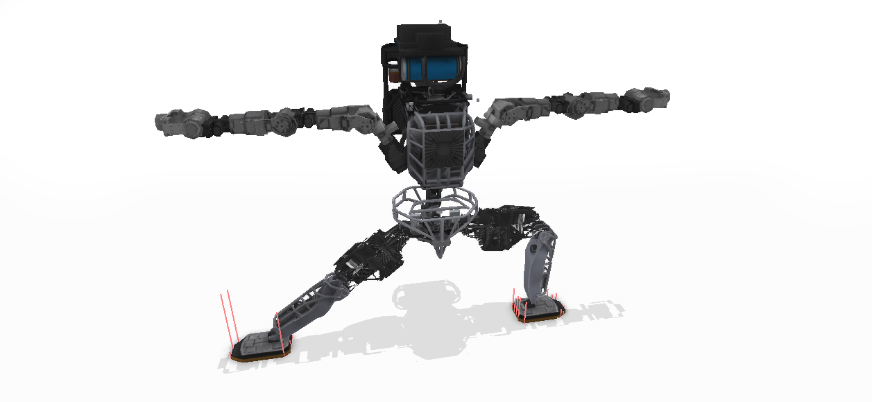
First, we evaluate our methods by testing the performance of gradient computation. In addition, we compare gradient-based trajectory optimization enabled by our method to gradient-free stochastic optimization, and discuss implications. We also demonstrate the effectiveness of the complementarity-aware gradients in a trajectory optimization problem. Finally, we show that our physics engine can solve optimal control problems for complex dynamic systems with contact and collision, including an Atlas humanoid jumping in the air.

We present a fast and feature-complete differentiable physics engine for articulated rigid body simulation. We introduce a method to compute analytical gradients through the LCP formulation of inelastic contact by exploiting the sparsity of the LCP solution. Our engine supports complex contact geometry and approximating continuous-time elastic collision. We also introduce a novel method to compute complementarity-aware gradients that help optimizers to avoid stalling in saddle points.

There a few limitations of our current method. Currently, computing $\frac{\partial\boldsymbol{J}_{t}\boldsymbol{f}}{\partial\boldsymbol{q}_{t}}$, the way the joint torques produced by the contact forces change as we vary joint positions (which in turn varies contact positions and normals) takes a large portion of the total time to compute all Jacobians of dynamics for a given timestep. Perhaps a more efficient formulation can be found.

Our engine also doesn’t yet differentiate through the geometric properties (like link length) of a robot, or friction coefficients. Extending to these parameters is an important step to enable parameter estimation applications.

We are excited about future work that integrates gradients and stochastic methods to solve hard optimization problems in robotics. In running the experiments for this paper, we found that stochastic trajectory optimization methods could often find better solutions to complex problems than gradient-based methods, because they were able to escape from local optima. However, stochastic methods are notoriously sample inefficient, and have trouble fine-tuning results as they begin to approach a local optima. The authors speculate that there are many useful undiscovered techniques waiting to be invented that lie at the intersection of stochastic gradient-free methods and iterative gradient-based methods. It is our hope that an engine like the one presented in this paper will enable such research.

References

- Al-Rfou et al. [2016] Rami Al-Rfou, Guillaume Alain, Amjad Almahairi, Christof Angermueller, Dzmitry Bahdanau, Nicolas Ballas, Frédéric Bastien, Justin Bayer, Anatoly Belikov, Alexander Belopolsky, et al. Theano: A python framework for fast computation of mathematical expressions. arXiv e-prints, pages arXiv–1605, 2016.
- Amos and Kolter [2017] Brandon Amos and J Zico Kolter. Optnet: Differentiable optimization as a layer in neural networks. In Proceedings of the 34th International Conference on Machine Learning-Volume 70, pages 136–145. JMLR. org, 2017.
- Baraff [1994] David Baraff. Fast contact force computation for nonpenetrating rigid bodies. In Proceedings of the 21st annual conference on Computer graphics and interactive techniques, pages 23–34, 1994.
- Battaglia et al. [2016] Peter Battaglia, Razvan Pascanu, Matthew Lai, Danilo Jimenez Rezende, et al. Interaction networks for learning about objects, relations and physics. In Advances in neural information processing systems, pages 4502–4510, 2016.
- Boutselis et al. [2020] George I Boutselis, Ziyi Wang, and Evangelos A Theodorou. Constrained sampling-based trajectory optimization using stochastic approximation. In 2020 IEEE International Conference on Robotics and Automation (ICRA), pages 2522–2528. IEEE, 2020.
- Boyd et al. [2003] Stephen Boyd, Lin Xiao, and Almir Mutapcic. Subgradient methods. lecture notes of EE392o, Stanford University, Autumn Quarter, 2004:2004–2005, 2003.
- Carpentier and Mansard [2018] Justin Carpentier and Nicolas Mansard. Analytical derivatives of rigid body dynamics algorithms. In Robotics: Science and Systems (RSS 2018), 2018.
- Chang et al. [2016] Michael B Chang, Tomer Ullman, Antonio Torralba, and Joshua B Tenenbaum. A compositional object-based approach to learning physical dynamics. arXiv preprint arXiv:1612.00341, 2016.
- Coumans [2010] Erwin Coumans. Bullet physics engine. Open Source Software: http://bulletphysics. org, 1(3):84, 2010.
- de Avila Belbute-Peres et al. [2018] Filipe de Avila Belbute-Peres, Kevin Smith, Kelsey Allen, Josh Tenenbaum, and J Zico Kolter. End-to-end differentiable physics for learning and control. In Advances in Neural Information Processing Systems, pages 7178–7189, 2018.
- Degrave et al. [2019] Jonas Degrave, Michiel Hermans, Joni Dambre, and Francis Wyffels. A differentiable physics engine for deep learning in robotics. Frontiers in neurorobotics, 13:6, 2019.
- Geilinger et al. [2020] Moritz Geilinger, David Hahn, Jonas Zehnder, Moritz Bächer, Bernhard Thomaszewski, and Stelian Coros. Add: analytically differentiable dynamics for multi-body systems with frictional contact. ACM Transactions on Graphics (TOG), 39(6):1–15, 2020.
- Hahn et al. [2019] David Hahn, Pol Banzet, James M. Bern, and Stelian Coros. Real2sim: Visco-elastic parameter estimation from dynamic motion. ACM Trans. Graph., 38(6), November 2019.
- Heiden et al. [2019] Eric Heiden, David Millard, Hejia Zhang, and Gaurav S Sukhatme. Interactive differentiable simulation. arXiv preprint arXiv:1905.10706, 2019.
- Heiden et al. [2020] Eric Heiden, David Millard, Erwin Coumans, and Gaurav S Sukhatme. Augmenting differentiable simulators with neural networks. arXiv preprint arXiv:2007.06045, 2020.
- Hermans et al. [2014] Michiel Hermans, Benjamin Schrauwen, Peter Bienstman, and Joni Dambre. Automated design of complex dynamic systems. PLOS ONE, 9(1):1–11, 01 2014.
- Holl et al. [2020] Philipp Holl, Nils Thuerey, and Vladlen Koltun. Learning to control pdes with differentiable physics. In International Conference on Learning Representations, 2020.
- Hu et al. [2019a] Yuanming Hu, Luke Anderson, Tzu-Mao Li, Qi Sun, Nathan Carr, Jonathan Ragan-Kelley, and Frédo Durand. Difftaichi: Differentiable programming for physical simulation. arXiv preprint arXiv:1910.00935, 2019a.
- Hu et al. [2019b] Yuanming Hu, Tzu-Mao Li, Luke Anderson, Jonathan Ragan-Kelley, and Frédo Durand. Taichi: a language for high-performance computation on spatially sparse data structures. ACM Transactions on Graphics (TOG), 38(6):1–16, 2019b.
- Hu et al. [2019c] Yuanming Hu, Jiancheng Liu, Andrew Spielberg, Joshua B Tenenbaum, William T Freeman, Jiajun Wu, Daniela Rus, and Wojciech Matusik. Chainqueen: A real-time differentiable physical simulator for soft robotics. Proceedings of IEEE International Conference on Robotics and Automation (ICRA), 2019c.
- Iollo et al. [2001] A. Iollo, M. Ferlauto, and L. Zannetti. An aerodynamic optimization method based on the inverse problem adjoint equations. Journal of Computational Physics, 173(1):87–115, 2001.
- Jacobson and Mayne [1970] David H Jacobson and David Q Mayne. Differential dynamic programming. 1970.
- Jarny et al. [1991] Y. Jarny, M.N. Ozisik, and J.P. Bardon. A general optimization method using adjoint equation for solving multidimensional inverse heat conduction. International Journal of Heat and Mass Transfer, 34(11):2911–2919, 1991.
- Jourdan et al. [1998] Franck Jourdan, Pierre Alart, and Michel Jean. A gauss-seidel like algorithm to solve frictional contact problems. Computer Methods in Applied Mechanics and Engineering, 155(1):31–47, 1998.
- Kim [2012] Junggon Kim. Lie group formulation of articulated rigid body dynamics. Technical report, Technical Report. Carnegie Mellon University, 2012.
- Lee et al. [2018] Jeongseok Lee, Michael X Grey, Sehoon Ha, Tobias Kunz, Sumit Jain, Yuting Ye, Siddhartha S Srinivasa, Mike Stilman, and C Karen Liu. Dart: Dynamic animation and robotics toolkit. Journal of Open Source Software, 3(22):500, 2018.
- Liang et al. [2019] Junbang Liang, Ming Lin, and Vladlen Koltun. Differentiable cloth simulation for inverse problems. In H. Wallach, H. Larochelle, A. Beygelzimer, F. d'Alché-Buc, E. Fox, and R. Garnett, editors, Advances in Neural Information Processing Systems, volume 32. Curran Associates, Inc., 2019.
- McNamara et al. [2004] Antoine McNamara, Adrien Treuille, Zoran Popović, and Jos Stam. Fluid control using the adjoint method. ACM Trans. Graph., 23(3):449–456, August 2004.
- Millard et al. [2020] David Millard, Eric Heiden, Shubham Agrawal, and Gaurav S. Sukhatme. Automatic differentiation and continuous sensitivity analysis of rigid body dynamics, 2020.
- Mrowca et al. [2018] Damian Mrowca, Chengxu Zhuang, Elias Wang, Nick Haber, Li F Fei-Fei, Josh Tenenbaum, and Daniel L Yamins. Flexible neural representation for physics prediction. In Advances in neural information processing systems, pages 8799–8810, 2018.
- Paszke et al. [2017] Adam Paszke, Sam Gross, Soumith Chintala, Gregory Chanan, Edward Yang, Zachary DeVito, Zeming Lin, Alban Desmaison, Luca Antiga, and Adam Lerer. Automatic differentiation in pytorch. 2017.
- Popović et al. [2000] Jovan Popović, Steven M. Seitz, Michael Erdmann, Zoran Popović, and Andrew Witkin. Interactive manipulation of rigid body simulations. In Proceedings of the 27th Annual Conference on Computer Graphics and Interactive Techniques, SIGGRAPH ’00, page 209–217. ACM Press/Addison-Wesley Publishing Co., 2000.
- Press et al. [2007] William H. Press, Saul A. Teukolsky, William T. Vetterling, and Brian P. Flannery. Numerical Recipes 3rd Edition: The Art of Scientific Computing. Cambridge University Press, USA, 3 edition, 2007.
- Qiao et al. [2020] Yi-Ling Qiao, Junbang Liang, Vladlen Koltun, and Ming C. Lin. Scalable differentiable physics for learning and control. In ICML, 2020.
- Rackauckas et al. [2018] Christopher Rackauckas, Yingbo Ma, Vaibhav Dixit, Xingjian Guo, Mike Innes, Jarrett Revels, Joakim Nyberg, and Vijay Ivaturi. A comparison of automatic differentiation and continuous sensitivity analysis for derivatives of differential equation solutions, 2018.
- Ridders [1982] C.J.F. Ridders. Accurate computation of f’(x) and f’(x) f”(x). Advances in Engineering Software (1978), 4(2):75–76, 1982.
- Schenck and Fox [2018] Connor Schenck and Dieter Fox. Spnets: Differentiable fluid dynamics for deep neural networks. In Proceedings of The 2nd Conference on Robot Learning, volume 87 of Proceedings of Machine Learning Research, pages 317–335. PMLR, 29–31 Oct 2018.
- Song and Boularias [2020] Changkyu Song and Abdeslam Boularias. Learning to slide unknown objects with differentiable physics simulations. In Robotics: Science and Systems, Oregon State University at Corvallis, Oregon, USA, 14–16 July 2020.
- Tassa et al. [2012] Yuval Tassa, Tom Erez, and Emanuel Todorov. Synthesis and stabilization of complex behaviors through online trajectory optimization. In 2012 IEEE/RSJ International Conference on Intelligent Robots and Systems, pages 4906–4913. IEEE, 2012.
- Todorov and Li [2005] Emanuel Todorov and Weiwei Li. A generalized iterative lqg method for locally-optimal feedback control of constrained nonlinear stochastic systems. In Proceedings of the 2005, American Control Conference, 2005., pages 300–306. IEEE, 2005.
- Todorov et al. [2012] Emanuel Todorov, Tom Erez, and Yuval Tassa. Mujoco: A physics engine for model-based control. In 2012 IEEE/RSJ International Conference on Intelligent Robots and Systems, pages 5026–5033. IEEE, 2012.
- Toussaint et al. [2018] Marc Toussaint, Kelsey R. Allen, K. Smith, and J. Tenenbaum. Differentiable physics and stable modes for tool-use and manipulation planning. In Robotics: Science and Systems, 2018.