Fast electromagnetic response of a thin film of resonant atoms with permanent dipole
Abstract
We consider the propagation of extremely short pulses through a dielectric thin film containing resonant atoms (two level atoms) with permanent dipole. Assuming that the film width is less than the field wave length, we can solve the wave equation and reduce the problem to a system of generalized Bloch equations describing the resonant atoms. We compute the stationary solutions for a constant irradiation of the film. Superimposing a small amplitude linear wave we compute the reflection and transmission coefficients. From these, one can then deduce the different parameters of the model. We believe this technique could be used in experiments to obtain the medium atomic and relaxation parameters.
1:Laboratoire de Mathématiques, INSA de Rouen,
B.P. 8, 76131 Mont-Saint-Aignan cedex, France
E-mail: caputo@insa-rouen.fr
2 Center for Engineering Science Advanced Research,
Computer Science and Mathematics Division,
Oak Ridge National Laboratory,
Oak Ridge, TN 37831, USA
E-mail: kazantsevaev@ornl.gov
3: Department of Solid State Physics and Nanosystems,
Moscow Engineering Physics Institute,
Kashirskoe sh. 31, Moscow 115409, Russia
E-mail: amaimistov@gmail.com
PACS numbers : 42.25.Bs, 42.65.Pc, 42.81.Dp
Keywords: thin film, two level atoms, permanent dipole, refractive phenomena
1 Introduction
One of the famous models describing field-matter interaction is the Maxwell-Bloch system [1]. It corresponds to an ensemble of two-level atoms whose states alternate due to the electromagnetic field. In a simple approach the electromagnetic field is assumed to be scalar and the operator of dipole transition to only have non-diagonal matrix elements. This model was the base for the description of many coherent nonlinear effects, the coherent pulse propagation (self-induced transparency [2]) and the coherent transient effects (optical nutations, free induction decay, quantum beats, superradiance, photon echo). A detailed review of these phenomena may be found in [3, 4] and in the book [1].
The Maxwell-Bloch system can be extended further than the model of two-level atoms discussed above. In particular one can generalize the resonant atomic model. The model of three-level atom now attracts great interest, because it describes electromagnetic induced transparency, slow light propagation in (three-level) atomic vapor [5] and the coherent population transfer [6]. The coherent interaction of electromagnetic pulses with quantum dots [7, 8] can be described by such a generalized Maxwell-Bloch system. Another generalization of the two-level model is to take into account diagonal matrix elements of the dipole transition operator [12]. In this medium steady state one-half cycle pulses were obtained in the sharp line limit [13]. A new kind of steady state pulse was found, characterized by an algebraic decay of the electric field.
The reduced Maxwell-Bloch equation in the sharp line limit have a zero-curvature representation[14, 15]. A number of results related with the complete integrability of this reduced system have been obtained in [16, 17, 18]. The numerical simulation of the propagation of extremely short pulses [19] shows the existence of an extraordinary breather with non zero pulse square. An analytical expression for this breather has been found in [14, 15] and reproduced in [20] using the Darboux transformation method. Recently Zabolotzki[21] developed the inverse scattering method to find the solution for the isotropic limit of the general model of a two-component electromagnetic field interacting with two-level atoms with a permanent dipole moment without invoking the slowly varying envelope approximation.
The influence of the permanent dipole on parametric processes was studied in [9, 10]. Recently Weifeng et al studied the generation of attosecond pulses in a two-level system with permanent dipole moment[11]. For this, higher harmonics are generated and the spectrum can be extended to the X-ray range. The quantum interference of both even and odd harmonics results in the generation of higher intensity attosecond pulses.
The propagation of ultrashort pulses propagation through a thin film containing resonant atoms located at the interface between two dielectrics is also described by the Maxwell-Bloch equations. However, if the width of the film is less than a wave length [22], the atomic system is compressed into a ”point”. An insightful comment was made in [23, 24], concerning the critical role of the local Lorentz field. This local field induces a nonlinearity so that the thin film of two-level atoms acts as a nonlinear Fabry-Perot resonator. One then expects optical bistability for this device. There are many generalizations of the thin film model, where three (or more) level atoms, two-photon transition between resonant levels and non-resonant nonlinearity were studied. Here we consider a thin film corresponding to two-level atoms with permanent dipole moment [25]. There the author analyzed numerically the pulse propagation through the film taking into account the local field. He showed that a dense film irradiated by a one-circle pulse emits a short response with a delay much longer than the characteristic cooperative time of the atom ensemble. Contrary to [25] we assume that the atoms of the film are rare so that the local field can be neglected.
Recently [28] we introduced a general formalism to describe
the interaction of a (linear polarized) electromagnetic pulse with a
medium. With this we studied a ferroelectric film
which was described by a Duffing oscillator naturally giving a double well
potential. Here we generalize this approach to the case of a layer
of resonant atoms described by the generalized Bloch equations
taking into account the permanent dipole moment. An important feature
of the model is that there is a clear separation between the medium
and the surrounding vacuum so that no dispersion relation can be written.
Instead we obtain a scattering problem where the reflection
and transmission coefficients need to be calculated.
After presenting the model in section 2, we compute its equilibria and
their stability
in section 3. In section 4 we assume an additional periodic
modulation around a fixed background field. This enables to do a
spectroscopy study of the film so that both the dipole parameter
and the coupling parameter can be extracted from the reflection
curve. Section 5 concludes the article.
2 The model
2.1 One dimensional wave propagation
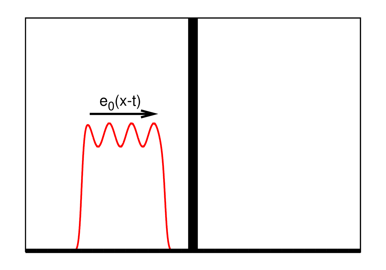
Following the formalism of [28] we assume that an electromagnetic wave is incident from the left on a medium whose position is given by the function . The configuration is shown in Fig. 1. Denoting by subscripts the partial derivatives, the equations are
| (1) | |||||
| (2) |
where is the polarization in the medium. Let the dielectric susceptibilities of surrounding mediums be the same. That eliminates the Fresnel refraction. The boundary conditions are
| (3) |
and the initial conditions are following the scattering problem. Then we have
| (4) |
We assume that the initial pulse is located at the left far from the film.
Using the general procedure for solving the wave equation (see [27]), we showed in [28] that the solution of this problem is
| (5) |
where we use the step-function
which can also be written as
When the medium is reduced to a single thin film placed at ,
The field at is given by
With this general formalism, one can address the question of what happens for a medium represented by an ensemble of resonant atoms. These could be molecules, quantum dots, or two or three level atoms. Here we will restrict ourselves to the two-level atoms with permanent dipole embedded into a thin film.
2.2 The case of a thin film of resonant atoms
Let the plane electromagnetic wave interact with the atoms or molecules characterized by the operator of the dipole transition between resonant energy levels and let this operator have both non-diagonal and diagonal matrix elements [12]. In the two-level approximation the Hamiltonian of the considered model can be written as[15]
where is the amplitude of the electric field of the electromagnetic wave and is the frequency difference between the levels. The polarization of the medium is
| (6) |
where is the film thickness and where is the volume density of the atoms. We assumed a homogeneous film and neglected the transverse dependence of . The atomic polarizability is given by the expression
| (7) |
where is the density matrix and where we used the constraint . In the expression above, the first term corresponds to the constant polarizability of the molecules. The average of this quantity over all atoms must be zero because we assume no polarization of the medium in the absence of an electromagnetic field. Note that all relaxation processes are neglected because we assume short electromagnetic pulses. We also neglect the dipole-dipole interaction, ie we assume the atoms carrying dipoles are rare in the film. The evolution of the elements of is given by the Heisenberg equation and yields the Bloch equations.
So the total system of equations describing the interaction of an electromagnetic wave with a collection of identical atoms in a film placed at is [12]
| (8) |
| (9) |
| (10) |
| (11) |
where are the components of the Bloch vector
| (12) |
In equations (9)-(11) the field is taken in the film, i.e., at . This system differs from the well-known Maxwell-Bloch equations [29, 30] by the terms containing the parameter .
We normalize time, space and electric field as
We also introduce the parameter which measures the strength of the permanent dipole:
| (13) |
Then the Maxwell-Bloch equations (8)-(11) take the form:
| (14) |
| (15) |
where , and
| (16) |
A rough estimation of this parameter taking 1 Debye gives so that for a film thickness of and a volume density we get . If the film is thinner, we can take the same range of with densities . This is still compatible with our hypothesis of dilute impurities in the medium so that we can neglect the dipole-dipole interaction.
The system can be further simplified by noting from equation (14) that . We then get
| (17) |
| (18) |
This is the model that we will analyze in detail in this article.
We will assume the general initial conditions where the medium is initially at rest so that , at . From the Bloch equations (14) we obtain and using the initial conditions we get the value of this integral of motion
| (19) |
We consider the effect of an electromagnetic pulse impinging on the thin film placed at . For that we can use the general result (5) to solve the wave equation (17). Taking the right part of (17) as a function under the integral in (5) we obtain the following expression
| (20) |
which represents the strength of the electrical field in the film. Now, using this expression we can write the modified Bloch equations as
| (21) | |||||
| (22) | |||||
| (23) |
These are the correct equations describing the resonant responses of two-level atoms of a thin film to an ultra-short electromagnetic pulse. It is worth noting that the electromagnetic wave is incident normally on the film. Second, all atoms of the film are identical. Finally note that we did not assume any limitation on the time duration of the electromagnetic pulse. It may be a half period pulse, i.e. an electromagnetic spike or a quasiharmonic wave.
Finally note that since the motion occurs on the Bloch sphere, the system (23) has the constraint . It is then natural to write it in the reduced coordinates such that
| (24) |
The system is then
| (25) | |||
| (26) |
3 Equilibrium states
We now study the stationary points of the system (23). Initially before the wave reaches it, the film is at rest. The electromagnetic field shifts the film state to a new equilibrium. The system then relaxes back to its original state after the wave has passed. We will examine these new transient states and their stability.
For constant, the system of equations (21-23) has the fixed point where satisfy
| (27) |
Assuming leads to a contradiction. From (19) it follows that
| (28) |
Combining these two equations we obtain
| (29) |
This fixed point corresponds to a stationary polarization and population induced in the two-level atoms by the incident constant field . When
| (30) |
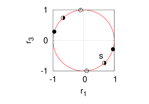
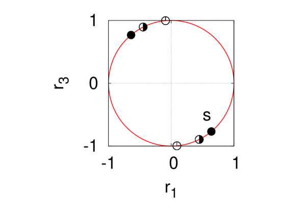
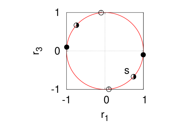
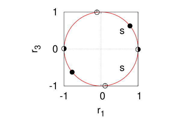
To understand geometrically the position of the fixed points, we can parametrize the Bloch sphere with by
yielding the relation
| (31) |
The dependence of the values on the electric field is monotonic so there is no bistability. The two fixed points are shown in Fig. 2 for . For small (left panel) the fixed points start from and rotate following with given by (31). For and so we obtain . Since is the difference in the population of the levels, these are equally populated. When is large and positive (top right panel) the fixed points do not change very much when the electric field is increased. On the contrary when is large and negative (bottom right panel) increasing the electric field shifts the fixed points from to for and about for . For this last value of the parameter we can have a strong population inversion.
To study the stability of the fixed point we linearize the modified Bloch equations. We set , , . The linearized modified Bloch equations read
| (32) | |||||
where as usual the subscript indicates the derivative. We introduce the field modified frequency
| (33) |
and ratio
| (34) |
From (32) we can get the equation for
| (35) |
The characteristic equation is
whose roots are
Then if and the fixed point is stable. Depending on two cases occur. Consider first a small so that . Then if , if . Then the fixed point such that is unstable. Conversely the fixed point such that is stable. If which occurs for and large fields the situation is reversed. The fixed point such that is stable while the one such that is unstable. The oscillation frequency of the orbit as it approaches the fixed point is given by the imaginary part of
| (36) |
.
When corresponding to a large , there is no imaginary part of . Even for very large the stability remains unchanged because for the first term will always dominate the second one . Therefore the fixed point such that is stable (resp. unstable) for (resp. ). In this case there are no oscillations around the fixed point.
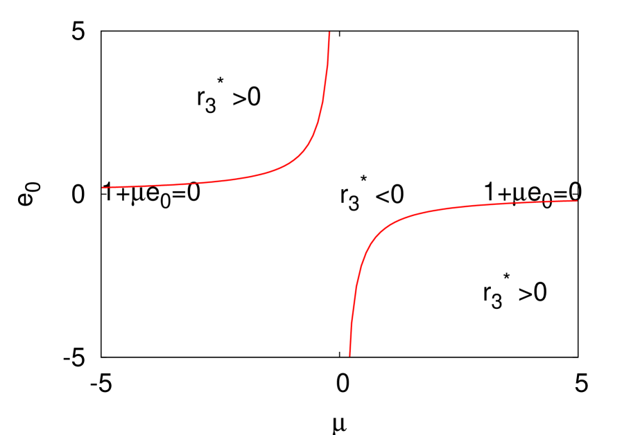
To conclude, for all values of , the stability is shown in Fig. 3 in the parameter space .
3.1 Numerical results
To illustrate the previous analysis, we have solved numerically the system of ordinary differential equations (21-23). We used the Runge-Kutta 4-5 Dopri5[34] as solver. For all the runs presented, we choose an incoming pulse
| (37) |
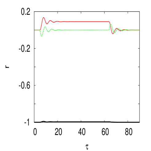
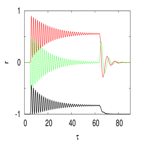
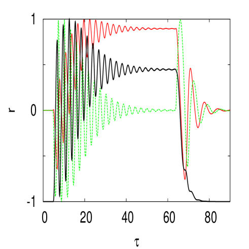
where , and . In the following we will abusively name the amplitude . We first consider . Fig. 4 shows the evolution of the Bloch vector components as a function of time, with from left to right and 2. As expected the system reaches the stable equilibrium state given by (29) with . The oscillations are given by the frequency and 3.6 from left to right. These plots correspond to the upper right panel of Fig. 2.
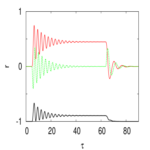
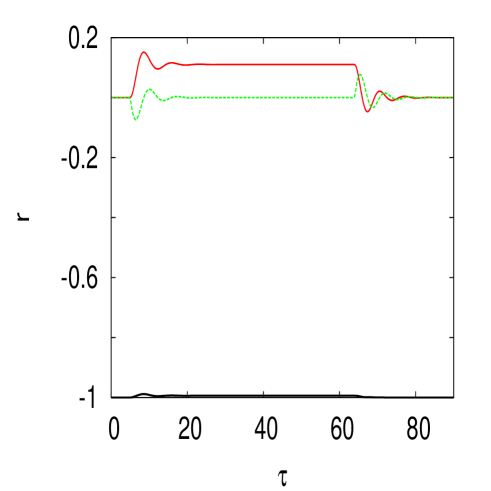
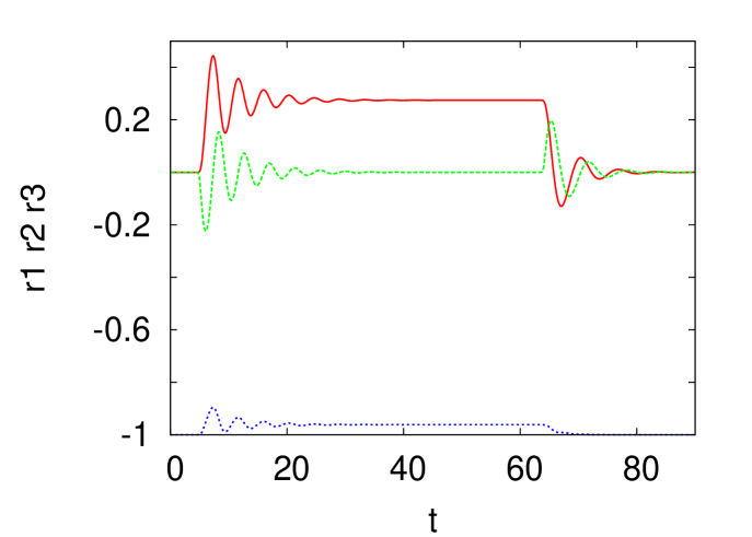
The case is shown in Fig. 5. When is small, we have an equilibrium very close to the one for as expected from the bottom right panel of Fig. 2. When we obtain the situation where and . Note the typical frequency as in the left panel. For a larger field , shown in the right panel we obtain as expected an equilibrium . Note the relatively small oscillation frequency compared for the one for the same and (right panel of Fig. 4).
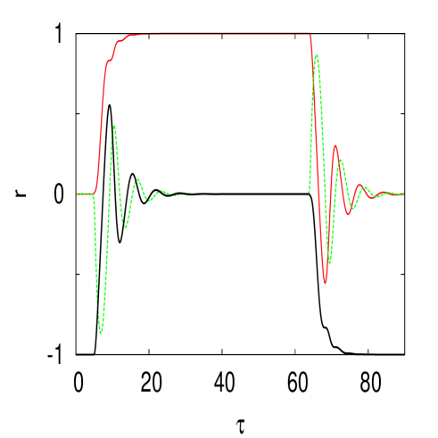
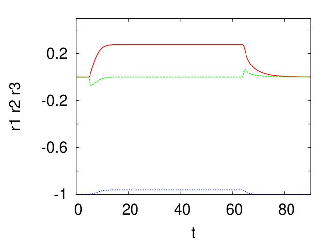
When is large, the fixed point does not change but the eigenvalue of the Jacobian is now real. We then get no oscillations as the system reaches the equilibrium as shown in the right panel of Fig. 6 for which and . Reducing to 1 restores the oscillations of frequency as shown in the left panel of Fig. 6.
4 Spectroscopic analysis of the film
We now assume a constant field applied to the film together with a small harmonic wave. It is then possible to examine how these waves of different frequencies get scattered by the film. Using this spectroscopic analysis of the film, we will see that one can recover the atomic dipolar parameter and the coupling parameter .
For a constant , the system (14,17) becomes
| (38) | |||||
| (39) | |||||
| (40) | |||||
| (41) |
where we temporarily use to define the Dirac delta function.
We separate time and space
| (42) |
and obtain the system
| (43) | |||||
| (44) | |||||
| (45) | |||||
| (46) |
From the second and fourth equations we get
| (47) |
Plugging these expression into (43) results in
| (48) |
where is given by (33). The substitution of the previous equation into (38) leads to the non standard eigenvalue problem
| (49) |
As usual we assume a scattering experiment so that the field is given by
| (52) |
At the film the field is continuous and its gradient satisfies the jump condition
| (55) |
where
Writing the two conditions (55) using the left and right fields results in
| (56) |
The solution is
The fixed point is such that , so that , so the reflection and transmission coefficients are
| (57) |
| (58) |
where the reflection and transmission coefficients satisfy From (29) we have
| (59) |
so that the transmission coefficient is
| (60) |
The modulus squared of the transmission and reflection coefficients are then
| (61) |
| (62) |
Let us examine how depends on the different parameters. It attains its maximum 1 for and decays at infinity as . The half-width of the resonance, such that can be easily obtained. Solving the quadratic equation for we get
| (63) |
for large . Therefore the half-width is
| (64) |
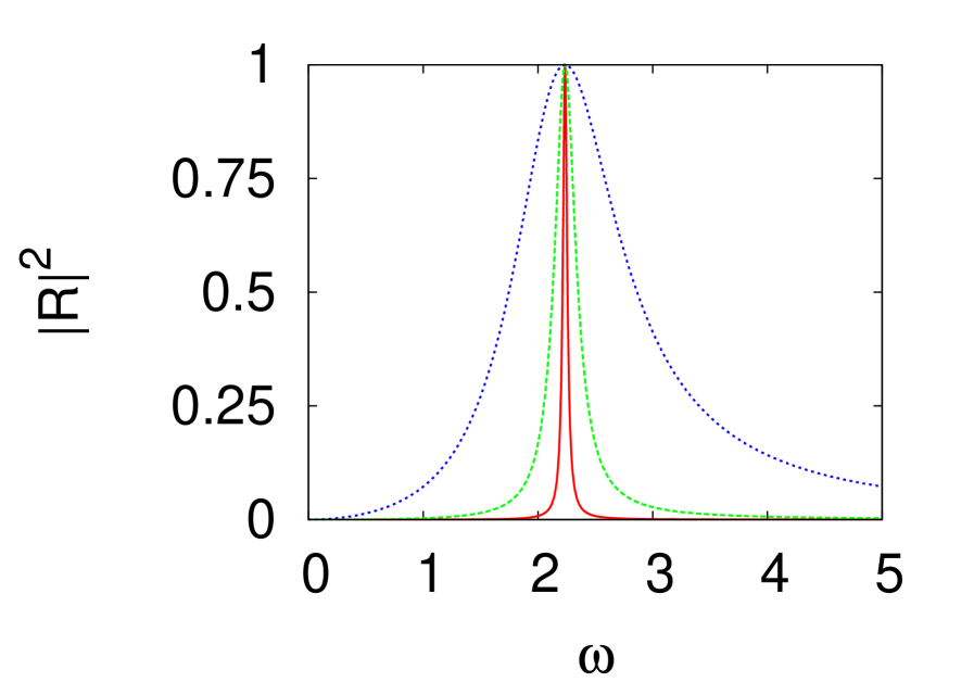
Fig. 7 shows the square of the modulus for a fixed (). As expected the half-width is proportional to . Notice how the resonance becomes asymmetric for large indicating that all higher order terms in (63) should be considered.
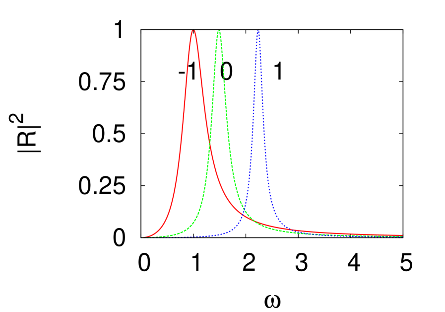
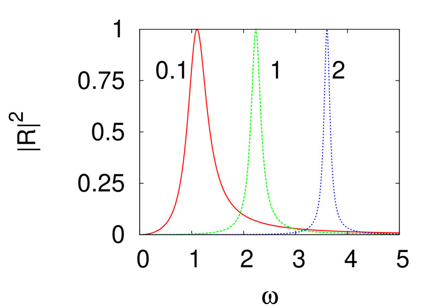
When is varied varies so will be shifted. Fig. 8 shows for and 1. As expected for (resp. ) the resonance is shifted towards low (resp. high) frequencies. For , the higher order terms in (63) should be taken into account and the resonance is not symmetric. When , the higher order terms can dropped and the resonance curve becomes symmetric.
The amplitude of the incoming pulse will also change the resonance by shifting . Fig. 9 shows for and 2. As expected, for the resonance is asymmetric. It becomes symmetric for .
5 Conclusion
We consider the electromagnetic pulse propagation thought the thin film containing the two-level atoms with taking account both non-diagonal and diagonal matrix elements of the operator of the dipole transition between resonant energy levels. The exact solution of the wave equation allows to derive the modified Bloch equations. Thus the problem of propagating extremely short (one- or few-cycle) pulses through a thin film is reduced to the analysis of a system of nonlinear ordinary differential equations on the Bloch sphere.
In the presence of a constant background field the equilibrium state of the system film/field is changed. These new equilibrium states are the fixed points of the modified Bloch equations. They depend on the field amplitude, the difference of diagonal elements of the operator of the dipole transition (dipole parameter) and the coupling constant. The stability analysis of these fixed points indicates which states will be attained by the system. For the stable states the population difference is negative or positive depending on the sign of the dipole parameter. When the film is illuminated by an electromagnetic field it reaches the new stable state with a typical relaxation time which depends on the field amplitude, the dipole parameter and the coupling constant. Using our estimate, experimentalists could measure the dipole parameter.
In the last part of the article we considered that in addition to a constant background, the thin film is irradiated by a small harmonic field of frequency . This spectroscopy analysis yields the reflection and transmission coefficients of the film as a function of . As expected the film is completely opaque i.e. its reflection coefficient is equal to 1 for the field modified transition frequency given by (33). We found that the width of the resonant curve is proportional to the coupling constant. The position of the resonance depends on the dipole parameter and the ground field.
The modern progress in nano-technology allows to produce thin films of different features and the investigation of such features is attractive. Our study shows that the fast electromagnetic response of a thin film could be used in experiments to measure intrinsic parameters of generalized atoms (quantum dots, meta-atoms, molecules …) and their coupling parameter to the field.
Acknowledgments
One of the authors (A.I.M.) is grateful to the Laboratoire de Mathématiques, INSA de Rouen for hospitality and support. Elena Kazantseva thanks the Region Haute-Normandie for a Post-doctoral grant. Jean-Guy Caputo thanks the Centre de Ressources Informatiques de Haute-Normandie for access to computing ressources. The authors express their gratitude to S.O. Elyutin for enlightening discussions.
References
- [1] L. Allen, J.H. Eberly, Optical Resonance and Two-Level Atoms, Wiley, N.Y. 1975).
- [2] S.L. McCall, E.L. Hahn, Phys.Rev.Lett. 18, 908 (1967); Phys.Rev.183, 457 (1969)
- [3] R.L.Shoemaker Ann.Rev.Phys.Chem. 30, 239-270 (1979)
- [4] A.I. Maimistov, A.M. Basharov, S.O. Elyutin, Yu.M. Sklyarov, Phys. Report 191, 1 (1990).
- [5] M.Fleischhauer, A.Imamoglu, and J.P. Marangos Rev.Mod. Phys. 77, 633-673 (2005)
- [6] K. Bergmann, H. Theuer, and B. W. Shore Rev.Mod.Phys. 70, 1003-1025 (1998)
- [7] S.O. Elyutin, E.V. Kazantseva, and A.I. Maimistov, Opt. Spectrosc. 90, 439-445 (2001)
- [8] A.I. Maimistov and S.O. Elyutin, Opt. Spectrosc. 93, 257-262 (2002).
- [9] J.P. Lavoine, C. Hoerner, A.A. Volleys, Phys.Rev. A 44, 5947 (1991)
- [10] R. Bavli, Y.B. Band, Phys.Rev. A 43, 5039 (1991),
- [11] Weifeng Yang, Shangqing Gong, Ruxin Li and Zhizhan Xu, Phys.Lett. A362, No. 1, 37-41 (2007)
- [12] L.W. Casperson, Phys. Rev. A,57 , 609-621 (1998).
- [13] A.I. Maimistov, J.-G. Caputo, Physica D 189, 107 (2004).
- [14] M. Agrotis, N.M. Ercolani, S.A. Glasgow, J.V. Moloney, Physica D 138. 134-162 (2000)
- [15] J. G. Caputo and A. I. Maimistov, Phys. Lett. A 296, 34-42, (2002).
- [16] M. Agrotis Physica D183, 141-158 (2003)
- [17] S.A. Glasgow, M.A. Agrotis, and N.M. Ercolani Physica D212, 82-99 (2005)
- [18] A.A. Zabolotski, Optics and Spectroscopy 95, 751-759 (2003).
- [19] S. O. Elyutin JETP 101, 11 (2005)
- [20] N. V. Ustinov, Proceedings SPIE, Vol. 6725 ICONO 2007: Nonlinear Space-Time Dynamics, Yuri Kivshar; Nikolay Rosanov, Editors, 67250F (2007); Breather-like pulses in a medium with the permanent dipole moment, arXiv: nlin.SI/0512056
- [21] A. A. Zabolotskii, J. Exp. Theor. Phys. 106, No. 5, 846-857 (2008)
- [22] V. I. Rupasov and V. I. Yudson, Sov. J. Quantum Electronics, 12, 415, (1982).
- [23] , M. G. Benedict, A. I. Zaitsev, V. A. Malyshev, and E.D. Trifonov, Opt. Spectrosk. 66, 726-728 (1989)
- [24] M. G. Benedict, V. A. Malishev, E.D. Trifonov and A. I. Zaitsev, Phys. Rev A 43, 3845, (1991).
- [25] S.O. Elyutin, Propagation of a videopulse through a thin layer of two-level dipolar atoms, J. Phys. B: At. Mol. Opt. Phys. 40, 2533-2550 (2007)
- [26] A.I. Maimistov, I.R. Gabitov, Nonlinear optical effects in artificial materials, Eur. Phys. J. Special Topics 147, 1, 265-286 (2007) in ”Nonlinear aves in complex systems: energy flow and geometry” (Springer, 2007)
- [27] A. N. Tikhonov and A. A. Samarski, Equations of Mathematical Physics (Dover, New York, 1983).
- [28] J.-G. Caputo, E. V. Kazantseva, A.I. Maimistov, Electromagnetically induced switching of ferroelectric thin films, Phys. Rev. B 75, 014113 (2007)
- [29] G.L.Lamb, Jr., Rev.Mod Phys. 43, 99- (1971).
- [30] R.K. Bullough, P.M. Jack, P.W. Kitchenside, R. Saudders , Phys.Scr. 20, 364- (1979).
- [31] F.T. Arecchi, E. Courtens, Phys.Rev. A 2, 1730 (1970)
- [32] N.E. Rehler, J.H. Eberly, Phys.Rev. A 3, 1735 (1971).
- [33] M.J. Ablowitz, H. Segur, Solitons and the Inverse Scattering Transformation, SIAM, Philadelphia, 1981.
- [34] E. Hairer, S. P. Norsett and G. Wanner. Solving ordinary differential equations I (Springer-Verlag, 1987).