Fast iterative method with a second order implicit difference scheme for time-space fractional convection-diffusion equations

Xian-Ming Gu^1,2, Ting-Zhu Huang¹, Cui-Cui Ji³,
Bruno Carpentieri⁴, Anatoly A. Alikhanov⁵
1. School of Mathematical Sciences,
University of Electronic Science and Technology of China,
Chengdu, Sichuan 611731, P.R. China
2. Institute of Mathematics and Computing Science, University of Groningen,
Nijenborgh 9, P.O. Box 407, 9700 AK Groningen, The Netherlands
3. Department of Mathematics,
Southeast University, Nanjing, Jiangsu 210096, P.R. China
4. School of Science and Technology,
Nottingham Trent University, Clifton Campus, Nottingham, NG11 8NS, UK
5. Institute of Applied Mathematics and Automation,
Russian Academy of Sciences, ul. Shortanova 89 a, Nalchik, 360000, Russia E-mail: guxianming@live.cn, x.m.gu@rug.nl.Corresponding author. E-mail: tingzhuhuang@126.com. Tel.: +86 28 61831608.E-mail: cuicuiahuan@163.com.E-mail: bcarpentieri@gmail.com.E-mail: aaalikhanov@gmail.com.

Abstract

In this paper we want to propose practical numerical methods to solve a class of initial-boundary problem of time-space fractional convection-diffusion equations (TSFCDEs). To start with, an implicit difference method based on two-sided weighted shifted Grünwald formulae is proposed with a discussion of the stability and convergence. We construct an implicit difference scheme (IDS) and show that it converges with second order accuracy in both time and space. Then, we develop fast solution methods for handling the resulting system of linear equation with the Toeplitz matrix. The fast Krylov subspace solvers with suitable circulant preconditioners are designed to deal with the resulting Toeplitz linear systems. Each time level of these methods reduces the memory requirement of the proposed implicit difference scheme from $\mathcal{O}(N^{2})$ to $\mathcal{O}(N)$ and the computational complexity from $O(N^{3})$ to $O(N\log N)$ in each iterative step, where $N$ is the number of grid nodes. Extensive numerical example runs show the utility of these methods over the traditional direct solvers of the implicit difference methods, in terms of computational cost and memory requirements.

Keywords: Fractional convection-diffusion equation; Shifted Grünwald discretization; Toeplitz matrix; Fast Fourier transform; Circulant preconditioner; Krylov subspace method.

AMSC (2010): 65F15, 65H18, 15A51.

1 Introduction

In recent years there has been a growing interest in the field of fractional calculus. Podlubny [1], Samko et al. [2] and Kilbas et al. [3] provide the history and a comprehensive treatment of this subject. Many phenomena in engineering, physics, chemistry and other sciences can be described very successfully by using fractional differential equations (FDEs). Diffusion with an additional velocity field and diffusion under the influence of a constant external force field are, in the Brownian case, both modelled by the convection-dispersion equation. In the case of anomalous diffusion this is no longer true, i.e., the fractional generalisation may be different for the advection case and the transport an external force field in [4]. In the study, we are very interested in the fast solver for solving the initial-boundary value problem of the time-space fractional convection-diffusion equation (TSFCDE) [5, 6]:

\begin{cases}\partial^{\alpha}_{0,t}u(x,t)=\gamma(t)\frac{\partial u(x,t)}{\partial x}+d_{+}(t){}_{a}D^{\beta}_{x}u(x,t)+d_{-}(t){}_{x}D^{\beta}_{b}u(x,t)+f(x,t),\\ u(x,0)=\phi(x),\qquad\qquad\quad a\leq x\leq b,\\ u(a,t)=u(b,t)=0,\qquad\quad 0<t\leq T,\\ \end{cases}

(1.1)

where $\alpha\in(0,1],~\beta\in(1,2],~a<x<b$ , and $0<t\leq T$ . Here, the parameters $\alpha$ and $\beta$ are the order of the TSFCDE, $f(x,t)$ is the source term, and diffusion coefficient functions $d_{\pm}(t)$ are non-negative under the assumption that the flow is from left to right. Moreover, the variable coefficients $\gamma(t)$ are real. The TSFCDE (1.1) can be regarded as generalizations of classical convection-diffusion equations with the first-order time derivative replaced by the Caputo fractional derivative of order $\alpha\in(0,1]$ , and the second-order space derivatives replaced by the two-sided Riemman-Liouville fractional derivative of order $\beta\in(1,2]$ . Namely, the time fractional derivative in (1.1) is the Caputo fractional derivative of order $\alpha$ [1] denoted by

\partial^{\alpha}_{0,t}u(x,t)=\frac{1}{\Gamma(1-\alpha)}\int^{t}_{0}\frac{\partial u(x,\xi)}{\partial\xi}\frac{d\xi}{(t-\xi)^{\alpha}},

(1.2)

and the left-handed ( ${}_{a}D^{\beta}_{x}$ ) and the right-handed ( ${}_{x}D^{\beta}_{b}$ ) space fractional derivatives in (1.1) are the Riemann-Liouville fractional derivatives of order $\beta$ [3, 2] which are defined by

{}_{a}D^{\beta}_{x}u(x,t)=\frac{1}{\Gamma(2-\beta)}\frac{\partial^{2}}{\partial x^{2}}\int^{x}_{a}\frac{u(\eta,t)d\eta}{(x-\eta)^{\beta-1}}

(1.3)

and

{}_{x}D^{\beta}_{b}u(x,t)=\frac{1}{\Gamma(2-\beta)}\frac{\partial^{2}}{\partial x^{2}}\int^{b}_{x}\frac{u(\eta,t)d\eta}{(\eta-x)^{\beta-1}},

(1.4)

where $\Gamma(\cdot)$ denotes the Gamma function. Truly, when $\alpha=1$ and $\beta=2$ , the above equation reduces to the classical convection-diffusion equation (CDE).

The fractional CDE has been recently treated by a number of authors. It is presented as a useful approach for the description of transport dynamics in complex systems which are governed by anomalous diffusion and non-exponential relaxation patterns [4, 5]. The fractional CDE is also used in groundwater hydrology research to model the transport of passive tracers carried by fluid flow in a porous medium [7]. Though analytic approaches, such as the Fourier transform method, the Laplace transform methods, and the Mellin transform method, have been proposed to seek closed-form solutions [1, 6, 8], there are very few FDEs whose analytical closed-form solutions are available. Therefore, the research on numerical approximation and techniques for the solution of FDEs has attracted intensive interest. Most early established numerical methods are developed for handling the space factional CDE or the time fractional CDE. For space fractional CDE, many researchers exploited the conventional shifted Grünwald discretization [9] and the implicit Euler (or Crank-Nicolson) time-step discretization for two-sided Riemman-Liouville fractional derivatives and the first order time derivative, respectively. Then they constructed many numerical treatments for space fractional CDE, refer to [9, 10, 11, 12, 16, 13, 14, 15, 17, 18] and references therein for details. Later, Chen and Deng combined the second-order discretization with the Crank-Nicolson temporal discretization for producing the novel numerical methods, which archive the second order accuracy in both time and space for space fractional CDE [19, 20]. Even Chen & Deng and Qu et al. separately designed the fast computational techniques, which can also reduce the required algorithmic storage, for implementing the above mentioned second order numerical method; see [20, 21] for details. Additionally, there are also some other interesting numerical methods for space fractional CDE, refer, e.g., to [22, 23, 24, 25, 26] for a discussion of these issues.

On the other hand, for time fractional CDE, many early implicit numerical methods are derived by the combination of the $L1$ approximate formula [27] for Caputo fractional derivative and the first/second order spatial discretization. These numerical methods are unconditionally convergent with the $\mathcal{O}(\tau^{2-\alpha}+h)$ or $\mathcal{O}(\tau^{2-\alpha}+h^{2})$ accuracy, where $\tau$ and $h$ are time-step size and spatial grid size, respectively. In order to improve the spatial accuracy, Cui [28, 29] and Mohebbi & Abbaszadeh [30] proposed, respectively, two compact exponential methods and a compact finite difference method for a time fractional convection-subdiffusion equation so that the spatial accuracy is improved to the fourth-order. However, the methods and analyses in [28, 30] are only for the equations with constant coefficients. In particular, the discussions in [30] are limited to a special time fractional convection-subdiffusion equation where the diffusion and convection coefficients are assumed to be one. In addition, some other related numerical methods have already been proposed for handling the time fractional CDE, see e.g. [31, 32, 33, 34, 35, 36] for details.

On contrast, although the numerical methods for space (or time) fractional CDE are extensively investigated in the past research, the work about numerically handling the TSFCDE is not too much. Firstly, Zhang [37, 38], Shao & Ma [39], Qin & Zhang [40], and Liu et al. [17] have worked out a series of studies about constructing the implicit difference scheme (IDS) for TSFCDE, however all these numerical scheme can archive the convergence with first order accuracy in both space and time from the both theoretical and numerical perspectives. Moreover, Liu et al. [41, 17], Zhao et al. [42], and Shen [43] had considered to solve the more general form of TSFCDE, in which the first-order space derivative is replaced by the two-sided Riemman-Liouville fractional derivative of order $\nu\in(0,1)$ . Again, their numerical methods cannot enjoy the convergence with second order accuracy in both space and time. In addition, some other efficient approaches are also developed for dealing with TSFCDE numerically. Moreover, most of these numerical methods have no complete theoretical analysis for both convergence and stability; e.g., refer to [44, 45, 46, 47, 24, 48, 49, 50] for details.

Traditional methods for solving FDEs tend to generate full coefficient matrices, which incur computational cost of $\mathcal{O}(N^{3})$ and storage of $O(N^{2})$ with $N$ being the number of grid points [14, 21]. To optimize the computational complexity, a shifted Grünwald discretization scheme with the property of unconditional stability was proposed by Meerschaet and Tadjeran [9] to approximate the space fractional CDE. Later, Wang and Wang [14] discovered that the linear system generated by this discretization has a special Toeplitz-like coefficient matrix, or, more precisely, this coefficient matrix can be expressed as a sum of diagonal-multiply-Toeplitz matrices. This implies that the storage requirement is $\mathcal{O}(N)$ instead of $\mathcal{O}(N^{2})$ , and the complexity of the matrix-vector multiplication only requires $\mathcal{O}(N\log N)$ operations by the fast Fourier transform (FFT) [51]. Upon using this advantage, Wang and Wang proposed the CGNR method having computational cost of $\mathcal{O}(N\log^{2}N)$ to solve the linear system and numerical experiments show that the CGNR method is fast when the diffusion coefficients are very small, i.e., the discretized systems are well-conditioned [14]. However, the discretized systems become ill-conditioned when the diffusion coefficients are not small. In this case, the CGNR method converges slowly. To remedy this shortcoming, Zhao et al. have extended the preconditioned technique, which is introduced by Lin et al. in the context of space fractional diffusion equation [52], for handling the Toeplitz-like linear systems coming from numerical discretization of TSFCDE [42]. Their results related to the promising acceleration of the convergence of the iterative methods, while solving (1.1).

In this paper, we firstly derive an implicit difference scheme for solving (1.1) and then verify that the proposed scheme can archive the stability and convergence with second order accuracy in both space and time (i.e. $\mathcal{O}(\tau^{2}+h^{2})$ ) from the both theoretical and numerical perspectives. As far as we know, the scheme is the first one (without extrapolation techniques) who can have the convergence with $\mathcal{O}(\tau^{2}+h^{2})$ . For the time marching of the scheme, plenty of linear systems, which possess different Toeplitz coefficient matrices, are required to be solved. Those linear systems can be solved efficiently one after one by using Krylov subspace method with suitable circulant preconditioners [51, 53], then it can reduce the computational cost and memory deeply. Especially for TSFCDE with constant coefficients, we turn to represent the inverse of the Toeplitz coefficient matrix as a sum of products of Toeplitz triangular matrices [51, 54], so that the solution of each linear system for time marching can be obtained directly via several fast Fourier transforms (FFTs). To obtain the explicit representation of Toeplitz matrix inversion, only two specific linear systems with the same Toeplitz coefficient matrix are needed to be solved, which can be done by using the preconditioned Krylov subspace methods [55] with complexity $O(N\log N)$ .

An outline of this paper is as follows. In Section 2, we establish an implicit difference scheme for (1.1) and prove that this scheme is unconditionally stable and convergent with $O(\tau^{2}+h^{2})$ order accuracy. In Section 3, we investigate that the resulting linear systems have the nonsymmetric Toeplitz matrices, then we design the fast solution techniques based on preconditioned Krylov subspace methods to solve (1.1) by exploiting the Toeplitz matrix property of the implicit difference scheme. Finally, we present numerical experiments to illustrate the effectiveness of our numerical approaches in Section 4 and provide concluding remarks in Section 5.

2 Implicit difference scheme

In this section, we present an implicit difference method for discretizing the TSFCDE defined by (1.1). Unlike former numerical approaches with the first order accuracy in both time and space [41, 42, 38, 37, 39], we exploit henceforth two-sided fractional derivatives to approximate the Riemann-Liouville derivatives in (1.3) and (1.4). We can show that, by two-sided fractional derivatives, this proposed method is also unconditionally stable and convergent under second order accuracy in time and space.

2.1 Numerical discretization of the TSFCDE

In order to derive the proposed scheme, we first introduce some notations. In the rectangle $\bar{Q}_{T}=\{(x,t):a\leq x\leq b,0\leq t\leq T\}$ we introduce the mesh $\varpi_{h\tau}=\varpi_{h}\times\varpi_{\tau}$ , where $\varpi_{h}=\{x_{i}=ih,~i=0,1,\ldots,N;~hN=b-a\}$ , and $\varpi_{\tau}=\{t_{j}=j\tau,~j=0,1,\ldots,M;~\tau=T/M\}$ . Besides, ${\bm{v}}=\{v_{i}\mid 0\leq i\leq N\}$ be any grid function. Then, the following lemma introduced in [56] gives a description on the time discretization.

Lemma 2.1

Suppose $0<\alpha<1$ , $\sigma=1-\frac{\alpha}{2},u(t)\in\mathcal{C}^{3}[0,T]$ , and $t_{j+\sigma}=(j+\sigma)\tau$ . Then

\partial^{\alpha}_{0,t_{j+\sigma}}u(t)-\Delta^{\alpha}_{0,t_{j+\sigma}}u(t)=\mathcal{O}(\tau^{3-\alpha}),

where $\Delta^{\alpha}_{0,t_{j+\sigma}}u(t)=\frac{\tau^{-\alpha}}{\Gamma(2-\alpha)}\sum^{j}_{s=0}c^{(\alpha,\sigma,j)}_{j-s}[u(t_{s+1})-u(t_{s})]$ , and $c^{(\alpha,\sigma,0)}_{0}=a^{(\alpha,\sigma)}_{0}$ for $j=0$ ,

c^{(\alpha,\sigma,j)}_{m}=\begin{cases}a^{(\alpha,\sigma)}_{0}+b^{(\alpha,\sigma)}_{1},&m=0,\\ a^{(\alpha,\sigma)}_{m}+b^{(\alpha,\sigma)}_{m+1}-b^{(\alpha,\sigma)}_{m},&1\leq m\leq j-1,\\ a^{(\alpha,\sigma)}_{j}-b^{(\alpha,\sigma)}_{j},&m=j,\\ \end{cases}

for $j\geq 1$ , in which $a^{(\alpha,\sigma)}_{0}=\sigma^{1-\alpha}$ , $a^{(\alpha,\sigma)}_{\ell}=(\ell+\sigma)^{1-\alpha}-(\ell-1+\sigma)^{1-\alpha},$ for $\ell\geq 1$ ; and $b^{(\alpha,\sigma)}_{\ell}=\frac{1}{2-\alpha}[(\ell+\sigma)^{2-\alpha}-(\ell-1+\sigma)^{2-\alpha}]-\frac{1}{2}[(\ell+\sigma)^{1-\alpha}+(\ell-1+\sigma)^{1-\alpha}]$ .

Denote $\mathfrak{L}^{n+\beta}(\mathbb{R})=\{v|v\in L_{1}(\mathbb{R})\ \mathrm{and}\ \int^{+\infty}_{-\infty}(1+|k|)^{n+\beta}|\hat{v}(k)|dk<\infty\}$ , where $\hat{v}(k)=\int^{+\infty}_{-\infty}e^{\iota kx}v(x)dx$ is the Fourier transformation of $v(x)$ , and we use $\iota=\sqrt{-1}$ to denote the imaginary unit. For the discretization on space, we introduce the following Lemma:

Lemma 2.2

([57, 58]) Suppose that $v\in\mathfrak{L}^{n+\beta}(\mathbb{R})$ , and let

\delta^{\beta}_{x,+}v(x)=\frac{1}{h^{\beta}}\sum^{[\frac{x-a}{h}]}_{k=0}\omega^{(\beta)}_{k}v(x-(k-1)h),

\delta^{\beta}_{x,-}v(x)=\frac{1}{h^{\beta}}\sum^{[\frac{b-x}{h}]}_{k=0}\omega^{(\beta)}_{k}v(x+(k-1)h),

then for a fixed $h$ , we have

{}_{a}D^{\beta}_{x}v(x)=\delta^{\beta}_{x,+}v(x)+\mathcal{O}(h^{2}),

{}_{x}D^{\beta}_{b}v(x)=\delta^{\beta}_{x,-}v(x)+\mathcal{O}(h^{2}),

where

\begin{cases}\omega^{(\beta)}_{0}=\lambda_{1}g^{(\beta)}_{0},\quad\ \omega^{(\beta)}_{1}=\lambda_{1}g^{(\beta)}_{1}+\lambda_{0}g^{(\beta)}_{0},\\ \omega^{(\beta)}_{k}=\lambda_{1}g^{(\beta)}_{k}+\lambda_{0}g^{(\beta)}_{k-1}+\lambda_{-1}g^{(\beta)}_{k-2},&k\geq 2,\end{cases}

with

\lambda_{1}=\frac{\beta^{2}+3\beta+2}{12},\quad\lambda_{0}=\frac{4-\beta^{2}}{6},\quad\lambda_{-1}=\frac{\beta^{2}-3\beta+2}{12},\quad and\ \ g^{(\beta)}_{k}=(-1)^{k}\binom{\beta}{k}.

Let $u(x,t)\in\mathcal{C}^{4,3}_{x,t}$ be a solution of the problem (1.1). Let us consider Eq. (1.1) for $(x,t)=(x_{i},t_{j+\sigma})\in\bar{Q}_{T},~i=1,2,\ldots,N-1,~j=0,1,\ldots,M-1,~\sigma=1-\frac{\alpha}{2}$ :

\begin{split}\partial^{\alpha}_{0,t_{j+\sigma}}u(x,t)=&~\gamma(t_{j+\sigma})\Big{(}\frac{\partial u(x,t)}{\partial x}\Big{)}_{(x_{i},t_{j+\sigma})}+d_{+}(t_{j+\sigma})\Big{(}{}_{a}D^{\beta}_{x}u(x,t)\Big{)}_{(x_{i},t_{j+\sigma})}+\\ &d_{-}(t_{j+\sigma})\Big{(}{}_{x}D^{\beta}_{b}u(x,t)\Big{)}_{(x_{i},t_{j+\sigma})}+f(x_{i},t_{j+\sigma}).\end{split}

For simplicity, let us introduce some notations

u^{(\sigma)}_{i}=\sigma u^{j+1}_{i}+(1-\sigma)u^{j}_{i},\quad\gamma^{(j+\sigma)}=\gamma(t_{j+\sigma}),\quad D^{(j+\sigma)}_{\pm}=d_{\pm}(t_{j+\sigma}),\quad f^{j+\sigma}_{i}=f(x_{i},t_{j+\sigma})

and

\delta^{\beta}_{h}u^{(\sigma)}_{i}=\gamma^{(j+\sigma)}\frac{u^{(\sigma)}_{i+1}-u^{(\sigma)}_{i-1}}{2h}+\frac{D^{(j+\sigma)}_{+}}{h^{\beta}}\sum^{i+1}_{k=0}\omega^{(\beta)}_{k}u^{(\sigma)}_{i-k+1}+\frac{D^{(j+\sigma)}_{-}}{h^{\beta}}\sum^{N-i+1}_{k=0}\omega^{(\beta)}_{k}u^{(\sigma)}_{i+k-1}.

Then with regard to Lemma 2.1 we derive the implicit difference scheme with the approximation order $\mathcal{O}(h^{2}+\tau^{2})$ :

\begin{cases}\Delta^{\alpha}_{0,t_{j+\sigma}}u_{i}=\delta^{\beta}_{h}u^{(\sigma)}_{i}+f^{j+\sigma}_{i},&1\leq i\leq N-1,\quad 0\leq j\leq M-1,\\ u^{0}_{i}=\phi(x_{i}),&1\leq i\leq N-1,\\ u^{j}_{0}=u^{j}_{N}=0,&0\leq j\leq M.\end{cases}

(2.1)

It is interesting to note that for $\alpha\rightarrow 1$ we obtain the Crank-Nicolson difference scheme.

2.2 Analysis of the implicit difference scheme

In this section, we analyze the stability and convergence for the implicit difference scheme (2.1). Let

V_{h}=\{{\bm{v}}\mid{\bm{v}}=\{v_{i}\}\ {\rm is}\ {\rm a}\ {\rm grid}\ {\rm function}\ {\rm on}\ \varpi_{h}\ {\rm and}\ v_{i}=0\ {\rm if}\ i=0,N\}

For $\forall{\bm{u}},~{\bm{v}}\in V_{h}$ , we define the discrete inner product and the corresponding discrete $L_{2}$ norm as follows,

({\bm{u}},{\bm{v}})=h\sum^{N-1}_{i=1}u_{i}v_{i},~~{\rm and}~~\|{\bm{u}}\|=\sqrt{({\bm{u}},{\bm{u}})}.

Now, some lemmas are provided for proving the stability and convergence of implicit difference scheme (2.1).

Lemma 2.3

([57, 9, 52]) Let $1<\alpha<2$ and $g^{(\beta)}_{k}$ be defined in Lemma 2.2. Then we have

\begin{cases}g^{(\beta)}_{0}=1,\quad g^{(\beta)}_{1}=-\beta,\quad g^{(\beta)}_{2}>g^{(\beta)}_{3}>\cdots>0,\\ \sum^{\infty}_{k=0}g^{(\beta)}_{k}=0,\quad\sum^{N}_{k=0}g^{(\beta)}_{k}<0,\quad\ N>1,\\ g^{(\beta)}_{k}=\mathcal{O}(k^{-(\beta+1)}),\quad\ g^{(\beta)}_{k}=\Big{(}1-\frac{\beta+1}{k}\Big{)}g^{(\beta)}_{k-1},\quad k=1,2,\ldots.\end{cases}

Lemma 2.4

([57, 58]) Let $1<\alpha<2$ and $g^{(\beta)}_{k}$ be defined in Lemma 2.2. Then we have

\begin{cases}\omega^{(\beta)}_{0}=1,\quad\omega^{(\beta)}_{1}<0,\quad\omega^{(\beta)}_{k}>0,\quad k\geq 3,\\ \sum^{\infty}_{k=0}\omega^{(\beta)}_{k}=0,\quad\sum^{N}_{k=0}\omega^{(\beta)}_{k}<0,\quad\ N>1,\\ \omega^{(\beta)}_{0}+\omega^{(\beta)}_{2}\geq 0.\end{cases}

Lemma 2.5

([57, 58]) For $1<\beta<2$ , and any ${\bm{v}}\in V_{h}$ , it holds that

(\delta^{\beta}_{x,+}{\bm{v}},{\bm{v}})=(\delta^{\beta}_{x,-}{\bm{v}},{\bm{v}})\leq\Big{(}\frac{1}{h^{\beta}}\sum^{N-1}_{k=0}\omega^{(\beta)}_{k}\Big{)}\|{\bm{v}}\|^{2}.

Lemma 2.6

For $1<\beta<2$ , $N\geq 5$ , and any ${\bm{v}}\in V_{h}$ , there exists a positive constant $c_{1}$ , such that

(-\delta^{\beta}_{x,+}{\bm{v}},{\bm{v}})=(-\delta^{\beta}_{x,-}{\bm{v}},{\bm{v}})>c_{1}\ln 2\|{\bm{v}}\|^{2}.

Proof. Since

\sum^{2N+2}_{k=N}\omega^{(\beta)}_{k}=\sum^{2N}_{k=N}g^{(\beta)}_{k}+(\lambda_{1}+\lambda_{0})g^{(\beta)}_{2N+1}+\lambda_{1}g^{(\beta)}_{2N+2}+\zeta(\beta),

where

\begin{split}\zeta(\beta)=(\lambda_{0}+\lambda_{-1})g^{(\beta)}_{N-1}+\lambda_{-1}g^{(\beta)}_{N-2}&=\Big{[}(\lambda_{0}+\lambda_{-1})\frac{N-2-\beta}{N-1}+\lambda_{-1}\Big{]}g^{(\beta)}_{N-2}\\ &=\frac{(12-6\beta)N+\beta^{3}+4\beta^{2}-\beta-22}{12(N-1)}g^{(\beta)}_{N-2},\\ &\triangleq\frac{\vartheta(\beta)}{12(N-1)}g^{(\beta)}_{N-2}\end{split}

then $\zeta(2)=0$ , $\vartheta(2)=0$ and $\vartheta^{\prime}(\beta)=-6N+3\beta^{2}+8\beta-1\leq 27-6N$ , which implies $\zeta(\beta)$ is a decreasing function for $\beta\in[1,2]$ , if $N\geq 5$ and $\vartheta^{\prime}(\beta)<0$ . Hence $\zeta(\beta)>0$ when $N\geq 5$ .

Then, by Lemma 2.3, there exist positive constants $\tilde{c}_{1}$ and $c_{1}$ , such that

\begin{split}\frac{1}{h^{\beta}}\sum^{\infty}_{k=N}\omega^{(\beta)}_{k}&>\frac{1}{h^{\beta}}\sum^{2N+2}_{k=N}\omega^{(\beta)}_{k}>\frac{1}{h^{\beta}}\sum^{2N}_{k=N}g^{(\beta)}_{k}\geq\tilde{c}_{1}\sum^{2N}_{k=N}k^{-(\beta+1)}N^{\beta}\\ &>\tilde{c}_{1}\sum^{2N}_{k=N}k^{-(\beta+1)}\Big{(}\frac{k}{2}\Big{)}^{\beta}\\ &=\frac{\tilde{c}_{1}}{2^{\beta}}\sum^{2N}_{k=N}\frac{1}{k}\geq c_{1}\int^{2N}_{N}\frac{1}{x}dx=c_{1}\ln 2,\quad\ N\geq 5.\end{split}

(2.2)

Using Lemmas 2.4 and 2.5, we then obtain

(-\delta^{\beta}_{x,+}{\bm{v}},{\bm{v}})=(-\delta^{\beta}_{x,-}{\bm{v}},{\bm{v}})>\Big{(}\frac{1}{h^{\beta}}\sum^{\infty}_{k=N}\omega^{(\beta)}_{k}\Big{)}\|{\bm{v}}\|^{2}>c_{1}\ln 2\|{\bm{v}}\|^{2},

which proves the lemma. $\Box$

Based on the above lemmas, we can obtain the following theorem, which is essential for analyzing the stability of the proposed implicit difference scheme.

Theorem 2.1

For any ${\bm{v}}\in V_{h}$ , it holds that

(\delta^{\beta}_{h}{\bm{v}},{\bm{v}})\leq-c\ln 2\|{\bm{v}}\|^{2},

where $c$ is a positive constant independent of the spatial step size $h$ .

Proof. The concrete expression of $(\delta^{\beta}_{h}{\bm{v}},{\bm{v}})$ can be written by

(\delta^{\beta}_{h}{\bm{v}},{\bm{v}})=\gamma^{(j+\sigma)}h\sum^{N-1}_{i=1}\frac{v_{i+1}-v_{i-1}}{2h}v_{i}+D^{(j+\sigma)}_{+}(\delta^{\beta}_{x,+}{\bm{v}},{\bm{v}})+D^{(j+\sigma)}_{-}(\delta^{\beta}_{x,-}{\bm{v}},{\bm{v}}).

(2.3)

It notes that $v^{0}=v^{N}=0$ , we have

\gamma^{(j+1)}h\sum^{N-1}_{i=1}\frac{v_{i+1}-v_{i-1}}{2h}v_{i}=0.

(2.4)

Moreover, according to Lemma 2.6, there exists a positive constant $c_{1}$ independent of the spatial step size $h$ , such that for any non-vanishing vector ${\bm{u}}\in V_{h}$ , we obtain

D^{(j+\sigma)}_{+}(\delta^{\beta}_{x,+}{\bm{v}},{\bm{v}})+D^{(j+\sigma)}_{-}(\delta^{\beta}_{x,-}{\bm{v}},{\bm{v}})\leq-c_{1}\ln 2\Big{(}D^{(j+\sigma)}_{+}+D^{(j+\sigma)}_{-}\Big{)}\|{\bm{v}}\|^{2}

(2.5)

Let $c=c_{1}\Big{(}D^{(j+\sigma)}_{+}+D^{(j+\sigma)}_{-}\Big{)}$ . Inserting (2.4) and (2.5) into (2.3), Theorem 2.1 holds. $\Box$

Lemma 2.7

([56, 58]) Let $V_{\tau}=\{{\bm{u}}|{\bm{u}}=(u^{0},u^{1},\ldots,u^{M})\}$ For any ${\bm{u}}\in V_{\tau}$ ; one has the following inequality

[\sigma u^{j+1}+(1-\sigma)u^{j}]\Delta^{\alpha}_{0,t_{j+\sigma}}{\bm{u}}\geq\frac{1}{2}\Delta^{\alpha}_{0,t_{j+\sigma}}({\bm{u}})^{2}.

Now we can conclude the stability and convergence of the implicit difference scheme (2.1). For simplicity of presentation, in our proof, we denote $a^{j+1}_{s}=\frac{c^{(\alpha,\sigma,j)}_{j-s}}{\tau^{\alpha}\Gamma(2-\alpha)}$ . Then $\Delta^{\alpha}_{0,t_{j+\sigma}}u=\sum^{j}_{s=0}(u^{s+1}-u^{s})a^{j+1}_{s}$ .

Theorem 2.2

Denote $\|f^{j+\sigma}\|^{2}=h\sum^{N-1}_{i=1}f^{2}(x_{i},t_{j+\sigma})$ . Then the implicit difference scheme (2.1) is unconditionally stable and the following a priori estimate holds:

\|u^{j+1}\|^{2}\leq\|u^{0}\|^{2}+\frac{T^{\alpha}\Gamma(1-\alpha)}{2c\ln 2}\|f^{j+\sigma}\|^{2},\quad\ 0\leq j\leq M-1,

(2.6)

where $u^{j+1}=(u^{j+1}_{1},u^{j+1}_{2},\ldots,u^{j+1}_{N-1})^{T}$ .

Proof. To make an inner product of (2.1) with $u^{(\sigma)}$ , we have

(\Delta^{\alpha}_{0,t_{j+\sigma}}u,u^{(\sigma)})=(\delta^{\beta}_{h}u^{(\sigma)},u^{(\sigma)})+(f^{j+\sigma},u^{(\sigma)}).

(2.7)

It follows from Theorem 2.1 and Lemma 2.6 that

	$\displaystyle(\delta^{\beta}_{h}u^{(\sigma)},u^{(\sigma)})\leq-c\ln 2\\|u^{(\sigma)}\\|^{2},$		(2.8)
	$\displaystyle(\Delta^{\alpha}_{0,t_{j+\sigma}}u,u^{(\sigma)})\geq\frac{1}{2}\Delta^{\alpha}_{0,t_{j+\sigma}}(\\|u\\|^{2}).$		(2.9)

Inserting (2.8)-(2.9) into (2.7) and using the Cauchy-Schwarz inequality, we obtain

\begin{split}\frac{1}{2}\Delta^{\alpha}_{0,t_{j+\sigma}}(\|u\|^{2})&\leq-c\ln 2\|u^{(\sigma)}\|^{2}+(f^{j+\sigma},u^{(\sigma)})\\ &\leq-c\ln 2\|u^{(\sigma)}\|^{2}+c\ln 2\|u^{(\sigma)}\|^{2}+\frac{1}{8c\ln 2}\|f^{j+\sigma}\|^{2}\\ &\leq\frac{1}{8c\ln 2}\|f^{j+\sigma}\|^{2}.\end{split}

(2.10)

Next, it holds that

a^{j+1}_{j}\|u^{j+1}\|^{2}\leq\sum^{j}_{s=1}(a^{j+1}_{s}-a^{j+1}_{s-1})\|u^{s}\|^{2}+a^{j+1}_{0}\|u^{0}\|^{2}+\frac{1}{4c\ln 2}\|f^{j+\sigma}\|^{2}.

Then, to notice that $a^{j+1}_{0}>\frac{1}{2T^{\alpha}\Gamma(1-\alpha)}$ (cf. [56]), we obtain

a^{j+1}_{j}\|u^{j+1}\|^{2}\leq\sum^{j}_{s=1}(a^{j+1}_{s}-a^{j+1}_{s-1})\|u^{s}\|^{2}+a^{j+1}_{0}\Big{(}\|u^{0}\|^{2}+\frac{T^{\alpha}\Gamma(1-\alpha)}{2c\ln 2}\|f^{j+\sigma}\|^{2}\Big{)}.

(2.11)

Suppose $h<1$ and denote

\check{\mathcal{P}}\triangleq\|u^{0}\|^{2}+\frac{T^{\alpha}\Gamma(1-\alpha)}{2c\ln 2}\|f^{j+\sigma}\|^{2}

Then, Eq. (2.11) can be rewritten by

a^{j+1}_{j}\|u^{j+1}\|^{2}\leq\sum^{j}_{s=1}(a^{j+1}_{s}-a^{j+1}_{s-1})\|u^{s}\|^{2}+a^{j+1}_{0}\check{\mathcal{P}}.

(2.12)

Next, we prove that the estimate relation (2.6) is valid for $j=0,1\ldots,M-1$ by mathematical induction. Obviously, It follows from (2.12) that (2.6) holds for $j=0$ . Let us assume that the inequality (2.6) takes place for all $0\leq j\leq k~(0\leq k\leq M-1)$ , that is

\|u^{j}\|\leq\check{\mathcal{P}},\qquad j=0,1,\ldots,k.

For (2.12) at $j=k$ , one has

\begin{split}a^{k+1}_{k}\|u^{k+1}\|^{2}&\leq\sum^{k}_{s=1}(a^{k+1}_{s}-a^{k+1}_{s-1})\|u^{s}\|^{2}+a^{k+1}_{0}\check{\mathcal{P}}\\ &\leq\sum^{k}_{s=1}(a^{k+1}_{s}-a^{k+1}_{s-1})\check{\mathcal{P}}+a^{k+1}_{0}\check{\mathcal{P}}=a^{k+1}_{k}\check{\mathcal{P}}.\end{split}

The proof of Theorem 2.2 is fully completed. $\Box$

Theorem 2.3

Suppose that $u(x,t)$ is the solution of (1.1) and $\{u^{j}_{i}\mid x_{i}\in\varpi_{h},~~0\leq j\leq M\}$ , is the solution of the implicit difference scheme (2.1). Denote

E^{j}_{i}=u(x_{i},t_{j})-u^{j}_{i},\quad x_{i}\in\varpi_{h},\quad 0\leq j\leq M.

Then there exists a positive constant $\tilde{c}$ such that

\|E^{j}\|\leq\tilde{c}(\tau^{2}+h^{2}),\quad\ 0\leq j\leq M.

Proof. It can easily obtain that $E^{j}$ satisfies the following error equation

\begin{cases}\Delta^{\alpha}_{0,t_{j+\sigma}}E_{i}=\delta^{\beta}_{h}E^{(\sigma)}_{i}=R^{j+\sigma}_{i},&1\leq i\leq N-1,\quad 0\leq j\leq M-1,\\ E^{0}_{i}=0,&1\leq i\leq N-1,\\ E^{j}_{0}=E^{j}_{N}=0,&0\leq j\leq M.\end{cases}

where $R^{j+\sigma}_{i}=\mathcal{O}(\tau^{2}+h^{2})$ . By exploiting Theorem 2.2, we get

\|E^{j+1}\|^{2}\leq\frac{T^{\alpha}\Gamma(1-\alpha)}{2c\ln 2}\|R^{j+\sigma}\|^{2}\leq\tilde{c}(\tau^{2}+h^{2}),\quad\ 0\leq j\leq M-1,

which proves the theorem. $\Box$

3 Fast solution techniques based on preconditioned iterative solvers

In the section, we contribute to establish the efficient methods for solving a group of linear systems with Toeplitz coefficient matrices, which are arisen from the matrix form of the implicit difference scheme (2.1). First of all, we derive the essential matrix form of the implicit difference scheme (2.1). Using notations in Section 2, the coefficient matrix of (2.1) corresponding to each time level $j$ can be written as the following form,

\begin{cases}\Big{[}\eta_{j}I-\sigma\Big{(}\frac{\gamma^{(\sigma)}}{2h}Q+\frac{D^{(\sigma)}_{+}}{h^{\beta}}W_{\beta}+\frac{D^{(\sigma)}_{-}}{h^{\beta}}W^{T}_{\beta}\Big{)}\Big{]}{\bm{u}}^{1}=\Big{[}\eta_{j}I+(1-\sigma)\Big{(}\frac{\gamma^{(\sigma)}}{2h}Q+\frac{D^{(\sigma)}_{+}}{h^{\beta}}W_{\beta}\\ +\frac{D^{(\sigma)}_{-}}{h^{\beta}}W^{T}_{\beta}\Big{)}\Big{]}{\bm{u}}^{0}+{\bm{f}}^{\sigma},\qquad\qquad\quad\ \ j=0,\\ \Big{[}\eta_{j}I-\sigma\Big{(}\frac{\gamma^{(j+\sigma)}}{2h}Q+\frac{D^{(j+\sigma)}_{+}}{h^{\beta}}W_{\beta}+\frac{D^{(j+\sigma)}_{-}}{h^{\beta}}W^{T}_{\beta}\Big{)}\Big{]}{\bm{u}}^{j+1}=\Big{[}\eta_{j}I+(1-\sigma)\Big{(}\frac{\gamma^{(j+\sigma)}}{2h}Q~+\\ \frac{D^{(j+\sigma)}_{+}}{h^{\beta}}W_{\beta}+\frac{D^{(j+\sigma)}_{-}}{h^{\beta}}W^{T}_{\beta}\Big{)}\Big{]}{\bm{u}}^{j}-\frac{\tau^{-\alpha}}{\Gamma(2-\alpha)}\sum\limits^{j-1}_{s=0}c^{(\alpha,\sigma,j)}_{j-s}({\bm{u}}^{s+1}-{\bm{u}}^{s})+{\bm{f}}^{j+\sigma},\\ \qquad\qquad\qquad\qquad\qquad\qquad\qquad\ \ j=1,2,\ldots,M-1,\end{cases}

(3.1)

where we have the coefficient

\eta_{j}=\begin{cases}\frac{c^{(\alpha,\sigma,0)}_{0}}{\tau^{\alpha}\Gamma(2-\alpha)}=\frac{a^{(\alpha,\sigma)}_{0}}{\tau^{\alpha}\Gamma(2-\alpha)},&j=0\\ \frac{c^{(\alpha,\sigma,j)}_{0}}{\tau^{\alpha}\Gamma(2-\alpha)}=\frac{a^{(\alpha,\sigma)}_{0}+b^{(\alpha,\sigma)}_{1}}{\tau^{\alpha}\Gamma(2-\alpha)},&j=1,2,\ldots,M-1,\end{cases}

then $Q$ and $W$ are two $(N-1)\times(N-1)$ real matrices of the following forms

Q=\begin{bmatrix}0&1&0&\cdots&0\\ -1&0&1&\ddots&\vdots\\ 0&-1&\ddots&\ddots&0\\ \vdots&\ddots&\ddots&\ddots&1\\ 0&\cdots&0&-1&0\end{bmatrix},\quad\ \ \ W_{\beta}=\begin{bmatrix}\omega^{(\beta)}_{1}&\omega^{(\beta)}_{0}&0&\cdots&0\\ \omega^{(\beta)}_{2}&\omega^{(\beta)}_{1}&\omega^{(\beta)}_{0}&\ddots&\vdots\\ \vdots&\omega^{(\beta)}_{2}&\omega^{(\beta)}_{1}&\ddots&0\\ \omega^{(\beta)}_{N-2}&\cdots&\ddots&\ddots&\omega^{(\beta)}_{0}\\ \omega^{(\beta)}_{N-1}&\omega^{(\beta)}_{N-2}&0&\omega^{(\beta)}_{2}&\omega^{(\beta)}_{1}\end{bmatrix}.

(3.2)

It is obvious that $W_{\beta}$ is a Toeplitz matrix (see [51, 14, 58]). Therefore, it can be stored with $N+1$ entries [51].

3.1 Resulting problems from the discretized scheme

According to (3.1) and (3.2), it indicates that the implicit difference scheme (2.1) requires to solve a nonsymmetric Toeplitz linear system in each time level $j$ , more precisely, there is a sequence of nonsymmetric Toeplitz linear systems

A^{(j+\sigma)}{\bm{u}}^{(j+1)}=B^{(j+\sigma)}{\bm{u}}^{(j)}+\delta{\bm{u}}^{(j)}+{\bm{f}}^{(j+\sigma)}

(3.3)

where $\delta{\bm{u}}^{(j)}$ is used to denote the calculation of $\frac{\tau^{-\alpha}}{\Gamma(2-\alpha)}\sum\limits^{j-1}_{s=0}c^{(\alpha,\sigma,j)}_{j-s}({\bm{u}}^{s+1}-{\bm{u}}^{s})$ and

	$\displaystyle A^{(j+\sigma)}=\eta_{j}I-\sigma\Big{(}\frac{\gamma^{(j+\sigma)}}{2h}Q+\frac{D^{(j+\sigma)}_{+}}{h^{\beta}}W_{\beta}+\frac{D^{(j+\sigma)}_{-}}{h^{\beta}}W^{T}_{\beta}\Big{)},$
	$\displaystyle B^{(j+\sigma)}=\eta_{j}I+(1-\sigma)\Big{(}\frac{\gamma^{(j+\sigma)}}{2h}Q+\frac{D^{(j+\sigma)}_{+}}{h^{\beta}}W_{\beta}+\frac{D^{(j+\sigma)}_{-}}{h^{\beta}}W^{T}_{\beta}\Big{)},$

$j=0,1,\ldots,M-1$ and $A^{(j+1)}$ varies with $j$ ; ${\bm{f}}^{(j+\sigma)}\in\mathbb{R}^{N-1}$ also varies with $j$ . Here it should highlight that the sequence of linear systems (3.3) corresponds to the time-stepping scheme (2.1), which is inherently sequential, hence the sequence of linear systems (3.3) is extremely difficult to parallelize over time.

On the other hand, it is remarkable that if the coefficients $\gamma(t)=\gamma$ and $d_{\pm}(t)=d_{\pm}$ , then the coefficient matrices

A^{(j+\sigma)}=\begin{cases}A^{(\sigma)},&j=0,\\ A,&j=1,2,\ldots,M-1.\end{cases}

(3.4)

Moreover, it is highlighted that the coefficient $\eta_{j}$ is a real constant, which does not vary with $j=1,2,\ldots,M-1$ . In other words, $A^{(j+\sigma)}=A=\eta_{j}I-\sigma\Big{(}\frac{\gamma}{2h}Q+\frac{d_{+}}{h^{\beta}}W_{\beta}+\frac{d_{-}}{h^{\beta}}W^{T}_{\beta}\Big{)}$ is independent of $j=1,\ldots,M-1$ , i.e. the coefficient matrix of (3.3) is unchanged in each time level ( $j=1,2,\ldots,M$ ) of the implicit difference scheme. In this case, if we still solve linear systems (3.3) one by one, it should be not sensible. A natural idea for this case is to find the inverse of the Toeplitz matrix $A$ , i.e. ${\bm{u}}=A^{-1}{\bm{f}}^{(j+\sigma)}$ . It means that we are interested in computing $A^{-1}$ once for all. One option is to compute the inverse by some direct methods such as the LU decomposition [60, pp. 44-54]. However, Toeplitz matrix is often dense, and the computation of the inverse of a large dense matrix is prohibitive, especially when the matrix is large. Fortunately, as $A$ is also a Toeplitz matrix, we have the Gohberg-Semencul formula (GSF) [51, 54] for its inverse. Indeed, the inverse of a Toeplitz matrix $A$ can be reconstructed from its first and last columns. More precisely, denote by ${\bm{e}}_{1},{\bm{e}}_{N-1}$ the first and the last column of the $(N-1)$ -by- $(N-1)$ identity matrix, and let ${\bm{x}}=[\xi_{0},\xi_{1},\ldots,\xi_{N-2}]^{T}$ and ${\bm{y}}=[\eta_{0},\eta_{1},\ldots,\eta_{N-2}]^{T}$ be the solutions of the following two Toeplitz systems

A{\bm{x}}={\bm{e}}_{1}\quad\ \mathrm{and}\quad\ A{\bm{y}}={\bm{e}}_{N-1}.

(3.5)

If $\xi_{0}\neq 0$ , then the Gohberg-Semencul formula can be expressed as

\begin{split}A^{-1}=&~\frac{1}{\xi_{0}}\Biggl{(}\begin{bmatrix}\xi_{0}&0&\cdots&0\\ \xi_{1}&\xi_{0}&\cdots&0\\ \vdots&\vdots&\ddots&\vdots\\ \xi_{N-2}&\xi_{N-3}&\cdots&\xi_{0}\\ \end{bmatrix}\cdot\begin{bmatrix}\eta_{N-2}&\eta_{N-3}&\cdots&\eta_{0}\\ 0&\eta_{N-2}&\cdots&\eta_{1}\\ \vdots&\vdots&\ddots&\vdots\\ 0&0&\cdots&\eta_{N-2}\\ \end{bmatrix}\\ &-\begin{bmatrix}0&0&\cdots&0\\ \eta_{0}&\cdots&0&0\\ \vdots&\vdots&\ddots&\vdots\\ \eta_{N-3}&\cdots&\eta_{0}&0\\ \end{bmatrix}\cdot\begin{bmatrix}0&\xi_{N-2}&\cdots&\xi_{1}\\ \vdots&\vdots&\ddots&\vdots\\ 0&0&\cdots&\xi_{N-2}\\ 0&0&\cdots&0\\ \end{bmatrix}\Biggr{)}=\frac{1}{\xi_{0}}(L_{p}R_{p}-L^{0}_{p}R^{0}_{p}),\end{split}

(3.6)

where $L_{p},~L^{0}_{p}$ are both lower Toeplitz matrices, and $R_{p},R^{0}_{p}$ are upper Toeplitz matrices. Consequently, the Toeplitz matrix-vector multiplication $A^{-1}{\bm{f}}^{(j+\sigma)}$ can be archived in several FFTs of length $N-1$ [51]. For convenience, the following fast algorithm can be applied to compute the product of $A^{-1}$ and a vector ${\bm{v}}$ .

Algorithm 1 Compute

{\bm{z}}=A^{-1}{\bm{v}}

1: Solve two linear systems in Eq. (3.5)

2: Compute

{\bm{z}}_{1}=R^{0}_{p}{\bm{v}}

and

{\bm{z}}_{2}=R_{p}{\bm{v}}

via FFTs

3: Compute

{\bm{z}}_{3}=L^{0}_{p}{\bm{z}}_{1}

and

{\bm{z}}_{4}=L_{p}{\bm{z}}_{2}

via FFTs

4: Compute

{\bm{z}}=\frac{1}{\xi_{0}}({\bm{z}}_{4}-{\bm{z}}_{3})

In summary, we need to search some efficient solvers for the nonsymmetric resulted Toeplitz linear systems, whether to solve (3.3) or to solve (3.5). In next subsection, we will introduce how to build efficient preconditioned iterative solvers for nonsymmetric Toeplitz linear systems.

3.2 Fast implementation of IDS based on preconditioned iterative solvers

In this subsection, we discuss the detailed framework about implementing the proposed implicit difference scheme (2.1). For the sake of clarity, an algorithm for solving the implicit difference scheme is given in Algorithm 2.

Algorithm 2 Practical implementation of IDS

1: for

j=0,1,\ldots,M-1

, do

2: Compute

{\bm{g}}^{(j+1)}=B^{(j+\sigma)}{\bm{u}}^{(j)}+\delta{\bm{u}}^{(j)}+{\bm{f}}^{(j+\sigma)}

3: Solve

A^{(j+\sigma)}{\bm{u}}^{(j+1)}={\bm{g}}^{(j+1)}

4: end for

From Algorithm 2, $M$ real linear systems are required to be solved. If a direct solver (e.g., Gaussian elimination method [60, pp. 33-44]) is applied, its complexity will be $\mathcal{O}(MN^{3})$ , which is very expansive if $N$ is large. Note that in Steps 2-3 of Algorithm 2, the Toeplitz structure of the matrices $A^{(j+\sigma)}$ and $B^{(j+\sigma)}$ has not been utilized when solving the linear system. Actually, the matrix-vector product $B^{(j+\sigma)}{\bm{u}}^{(j)}$ in Step 2 can be evaluated by FFTs in $\mathcal{O}(N\log N)$ operations, then fast Toeplitz iterative solvers have been studied intensively, see e.g., [51] and references therein. Recently, they have been applied for space fractional diffusion equation [52, 58, 59, 42, 14, 53]. With Krylov subspace method with circulant preconditioners in [53], the Toeplitz system from space fractional diffusion equation can be solved with a fast convergence rate. In this case, it also remarked that the algorithmic complexity of preconditioned Krylov subspace methods is only in $\mathcal{O}(N\log N)$ arithmetic operations per iteration step.

Motivated by the above considerations, we first implement the matrix-vector multiplication $B^{(j+\sigma)}{\bm{u}}^{(j)}$ in Step 1 of Algorithm 2 by FFTs. Then solving the Toeplitz linear systems $A^{(j+\sigma)}{\bm{u}}^{(j+1)}={\bm{g}}^{(j+1)}$ in Step 3 by Krylov subspace methods, e.g., the conjugate gradient squared (CGS) method [55, pp. 241-244], with the circulant preconditoner

P^{(j+\sigma)}=\eta_{j}I-\sigma\Big{(}\frac{\gamma^{(j+\sigma)}}{2h}s(Q)+\frac{D^{(j+\sigma)}_{+}}{h^{\beta}}s(W_{\beta})+\frac{D^{(j+\sigma)}_{-}}{h^{\beta}}s(W^{T}_{\beta})\Big{)},

(3.7)

where $s(\cdot)$ means the well-known Strang circulant approximation of a given Toeplitz matrix [51, 53]. High efficiency of Strang circulant preconditioner for space FDEs has been verified in [53]. To make sure the preconditioner defined in (3.7) is well-defined, let us illustrate that $P^{(j+\sigma)}$ are nonsingular,

Lemma 3.1

All eigenvalues of $s(W_{\beta})$ and $s(W^{T}_{\beta})$ fall inside the open disc

\{z\in\mathbb{C}:|z-\omega^{(\beta)}_{1}|<-\omega^{(\beta)}_{1}\}

(3.8)

Proof. All the Gershgorin disc [55, pp. 119-122] of the circulant matrices $s(W_{\beta})$ and $s(W^{T}_{\beta})$ are centered at $-\omega^{(\beta)}_{1}>0$ with radius

r_{N}=\omega^{(\beta)}_{0}+\sum^{\frac{\lfloor N\rfloor}{2}}_{k=2}\omega^{(\beta)}_{k}<\sum^{\infty}_{k=0,k\neq 1}\omega^{(\beta)}_{k}=-\omega^{(\beta)}_{1}.

(3.9)

by the properties of the sequence $\{\omega^{(\beta)}_{k}\}$ ; refer to Lemma 2.3 and Lemma 2.4. $\Box$

Remark 3.1

It is worth to mention that:

1.

The real parts of all eigenvalues of $s(W_{\beta})$ and $s(W^{T}_{\beta})$ are strictly negative for all $N$ ;
2.

The absolute values of all eigenvalues of $s(W_{\beta})$ and $s(W^{T}_{\beta})$ are bounded above by $2|\omega^{(\beta)}_{1}|$ for all $N$ .

As we know, a circulant matrix can be quickly diagonalized by the Fourier matrix $F$ [51, 21, 53]. Then it follows that $s(Q)=F^{*}\Lambda_{q}F$ , $s(W_{\beta})=F^{*}\Lambda_{\beta}F$ , and $s(W^{T}_{\beta})=F^{*}\bar{\Lambda}_{\beta}F$ , where $\bar{\Lambda}_{\beta}$ is the complex conjugate of $\Lambda_{\beta}$ . Decompose the circulant matrix $P^{(j+\sigma)}=F^{*}\Lambda_{p}F$ with the diagonal matrix $\Lambda_{p}=\eta_{j}I-\sigma\Big{(}\frac{\gamma^{(j+\sigma)}}{2h}\Lambda_{q}+\frac{D^{(j+\sigma)}_{+}}{h^{\beta}}\Lambda_{\beta}+\frac{D^{(j+\sigma)}_{-}}{h^{\beta}}\bar{\Lambda}_{\beta}\Big{)}$ . Then $P^{(j+\sigma)}$ is invertible if all diagonal entries of $\Lambda_{p}$ are nonzero. Moreover, we can obtain the following conclusion about the invertibility of $P^{(j+\sigma)}$ in (3.7).

Theorem 3.1

The circulant preconditioners $P^{(j+\sigma)}$ defined as in (3.7) are nonsingular.

Proof. First of all, we already know that $Q$ is a skew-symmetric Toeplitz matrix, it also finds that $s(Q)$ is also a skew-symmetric circulant matrix, thus the real part $\Lambda_{q}$ is equal to zero, i.e., $\mathrm{Re}([\Lambda_{q}]_{k,k})=0$ . On the other hand, by Part 1 of Remark 3.1, we have $\mathrm{Re}([\Lambda_{\beta}]_{k,k})<0$ . Noting that $\eta_{j}>0$ , $\sigma>0$ , and $D^{(j+\sigma)}_{\pm}\geq 0$ , thus we obtain

\mathrm{Re}([\Lambda_{p}]_{k,k})=\eta_{j}-\sigma\Big{(}0+\frac{D^{(j+\sigma)}_{+}}{h^{\beta}}\mathrm{Re}([\Lambda_{\beta}]_{k,k})+\frac{D^{(j+\sigma)}_{-}}{h^{\beta}}\mathrm{Re}([\bar{\Lambda}_{\beta}]_{k,k})\Big{)}\neq 0,

for each $k=1,2,\ldots,N-1$ . Therefore, $P^{(j+\sigma)}$ are invertible. $\Box$

Here although we do not plan to theoretically investigate the eigenvalue distributions of preconditioned matrices $(P^{(j+\sigma)})^{-1}A^{(j+\sigma)}$ , we still can give some figures to illustrate the clustering eigenvalue distributions of several specified preconditioned matrices in next section. Furthermore, our numerical experiments show that the iteration numbers always fluctuates between 6 and 10, so we regard the complexity of solving the linear system in Step 3 as $\mathcal{O}(N\log N)$ . It also implies that the computational complexity for implementing the whole IDS is about $\mathcal{O}(MN\log N)$ operations.

Beside, if we have the coefficients $\gamma(t)=\gamma$ and $d_{\pm}(t)=d_{\pm}$ in Eq. (1.1), the matrix $B^{(j+\sigma)}$ also has the similar form as $B^{(j+\sigma)}$ in Eq. (3.4), then we can simplify Algorithm 2 as the following Algorithm 3.

Algorithm 3 Practical implementation of IDS with constant coefficients

1: for

j=0,1,\ldots,M-1

, do

2: if

j=0

then

3: Compute

{\bm{g}}^{(1)}=B^{(\sigma)}{\bm{u}}^{(0)}+{\bm{f}}^{(\sigma)}

4: Solve

A^{(\sigma)}{\bm{u}}^{(1)}={\bm{g}}^{(1)}

5: else

6: Compute

{\bm{g}}^{(j+1)}=B{\bm{u}}^{(j)}+\delta{\bm{u}}^{(j)}+{\bm{f}}^{(j+\sigma)}

7: Solve

{\bm{u}}^{(j+1)}=A^{-1}{\bm{g}}^{(j+1)}

8: end if

9: end for

Again, if a direct method is employed to solve the linear system in Step 4 and compute matrix inverse $A^{-1}$ with the help of LU decomposition¹¹1For the given linear system $A{\bm{x}}={\bm{b}}$ , we solve it by MATLAB as: $\mathtt{[L,U]=lu(A);~~x=U\backslash(L\backslash b);}$ , which can be reused in Step 7 of Algorithm 3, but its complexity will be still $\mathcal{O}(MN^{3})$ , which is very costly if $N$ is large. Observe that in Steps 3, 4, 6 and 7 of Algorithm 3, the Toeplitz structure of those four matrices has not been utilized when solving the linear system. Actually, two matrix-vector multiplications $B^{(\sigma)}{\bm{u}}^{(0)}$ and $B{\bm{u}}^{(j)}$ in Steps 3 and 6 can be evaluated by FFTs in $\mathcal{O}(N\log N)$ operations, then fast Toeplitz iterative solvers with suitable circulant preconditioners, the Toeplitz system in Step 4 and (3.5) can be solved with a fast convergence rate. Here we can construct two circulant preconditioners defined as

	$\displaystyle P^{(\sigma)}=\eta_{0}I-\sigma\Big{(}\frac{\gamma}{2h}s(Q)+\frac{D_{+}}{h^{\beta}}s(W_{\beta})+\frac{D_{-}}{h^{\beta}}s(W^{T}_{\beta})\Big{)},$		(3.10)
	$\displaystyle P=\eta_{j}I-\sigma\Big{(}\frac{\gamma}{2h}s(Q)+\frac{D_{+}}{h^{\beta}}s(W_{\beta})+\frac{D_{-}}{h^{\beta}}s(W^{T}_{\beta})\Big{)},$		(3.11)

for the linear systems in Step 4 and (3.5), respectively. Here the invertibility of those above two circulant preconditioners introduced in (3.10)-(3.11) can be similarly archived by using Theorem 3.1. Then we can employ Algorithm 1 to evaluate the matrix-vector multiplication $A^{-1}{\bm{g}}^{(j+1)}$ in Step 7 of Algorithm 3. Similarly, according to results in next section, we find that the iteration numbers required by preconditioned Krylov subspace methods always fluctuate between 6 and 10. In this case, it also is remarkable that the algorithmic complexity of preconditioned Krylov subspace methods is only $\mathcal{O}(N\log N)$ at each iteration step. In conclusion, the total complexity for implementing the IDS with constant coefficients is also in $\mathcal{O}(MN\log N)$ operations.

4 Numerical results

In this section we first carry out some numerical experiments to illustrate that our proposed IDS can indeed converge with the second order accuracy in both space and time. At the same time, some numerical examples are reported to show the effectiveness of the fast solution techniques (i.e., Algorithms 1-3) designed in Section 3. For Krylov subspace method and direct solver, we choose built-in functions for the preconditioned CGS (PCGS) method, LU factorization of MATLAB in Example 1 and MATLAB’s backslash in Example 2, respectively. For the CGS method with circulant preconditioners, the stopping criterion of those methods is $\|{\bm{r}}^{(k)}\|_{2}/\|{\bm{r}}^{(0)}\|_{2}<10^{-12}$ , where ${\bm{r}}^{(k)}$ is the residual vector of the linear system after $k$ iterations, and the initial guess is chosen as the zero vector. All experiments were performed on a Windows 7 (64 bit) PC-Intel(R) Core(TM) i5-3740 CPU 3.20 GHz, 8 GB of RAM using MATLAB 2014a with machine epsilon $10^{-16}$ in double precision floating point arithmetic.

Example 1. In this example, we consider the equation (1.1) on space interval $[a,b]=[0,1]$ and time interval $[0,T]=[0,1]$ with diffusion coefficients $d_{+}(t)=d_{+}=0.8,~d_{-}(t)=d_{-}=0.5$ , convection coefficient $\gamma(t)=\gamma=-0.1$ , initial condition $u(x,0)=x^{2}(1-x)^{2}$ , and source term

\begin{split}f(x,t)=&~\frac{\Gamma(3+\alpha)}{2}x^{2}(1-x)^{2}t^{2}-(t^{2+\alpha}+1)\Big{\{}2\gamma x(1-x)(1-2x)+\frac{\Gamma(3)}{\Gamma(3-\beta)}[d_{+}x^{2-\beta}\\ &+d_{-}(1-x)^{2-\beta}]-\frac{2\Gamma(4)}{\Gamma(4-\beta)}[d_{+}x^{3-\beta}+d_{-}(1-x)^{3-\beta}]+\frac{\Gamma(5)}{\Gamma(5-\beta)}[d_{+}x^{4-\beta}\\ &+d_{-}(1-x)^{4-\beta}]\Big{\}}.\end{split}

The exact solution of this example is $u(x,t)=(t^{2+\alpha}+1)x^{2}(1-x)^{2}$ . For the finite difference discretization, the space step and time step are taken to be $h=1/N$ and $\tau=h$ , respectively. The errors ( $E=U-u$ ) and convergence order (CO) in the norms $\|\cdot\|_{0}$ and $\|\cdot\|_{\mathcal{C}(\bar{\omega}_{h\tau})}$ , where $\|U\|_{\mathcal{C}(\bar{\omega}_{h\tau})}=\max_{(x_{i},t_{j})\in\bar{\omega}_{h\tau}}|U|$ , are given in Tables 1-2. Here these notations are used throughout this section. Additionally, the performance of fast solution techniques presented in Section 3 for this example will be illustrated in Tables 3-4. In the following tables “Speed-up” is defined as

{\tt Speed\texttt{-}up}=\frac{\mathtt{Time1}}{\mathtt{Time2}}.

Obviously, when ${\tt Speed\texttt{-}up}>1$ , it means that Time2 needed by our proposed method is more competitive than Time1 required by Algorithm 3 with reusing LU decomposition in aspects of the CPU time elapsed.

Table 1:

L_{2}

-norm and maximum norm error behavior versus grid size reduction when

\tau=h

and

\beta=1.8

in Example 1.

$\alpha$	$h$	$\max_{0\leq n\leq M}\\|E^{n}\\|_{0}$	CO in $\\|\cdot\\|_{0}$	$\\|E\\|_{\mathcal{C}(\bar{\omega}_{h\tau})}$	CO in $\\|\cdot\\|_{\mathcal{C}(\bar{\omega}_{h\tau})}$
0.10	1/32	2.7954e-4	–	4.0880e-4	–
	1/64	6.6775e-5	2.0657	9.8580e-5	2.0520
	1/128	1.6010e-5	2.0603	2.3815e-5	2.0494
	1/256	3.8514e-6	2.0556	5.7630e-6	2.0470
0.50	1/32	2.6670e-4	–	3.8874e-4	–
	1/64	6.3583e-5	2.0685	9.3590e-5	2.0544
	1/128	1.5219e-5	2.0628	2.2573e-5	2.0518
	1/256	3.6558e-6	2.0576	5.4539e-6	2.0492
0.90	1/32	2.4972e-4	–	3.6255e-4	–
	1/64	5.9441e-5	2.0708	8.7173e-5	2.0562
	1/128	1.4206e-5	2.0650	2.0993e-5	2.0540
	1/256	3.4078e-6	2.0596	5.0762e-6	2.0481
0.99	1/32	2.5899e-4	–	3.7959e-4	–
	1/64	6.2121e-5	2.0598	9.1923e-5	2.0460
	1/128	1.4944e-5	2.0555	2.2275e-5	2.0450
	1/256	3.6057e-6	2.0512	5.4042e-6	2.0433

Table 2:

L_{2}

-norm and maximum norm error behavior versus

\tau

-grid size reduction when

h=1/1000

and

\beta=1.8

in Example 1.

$\alpha$	$\tau$	$\max_{0\leq n\leq M}\\|E^{n}\\|_{0}$	CO in $\\|\cdot\\|_{0}$	$\\|E\\|_{\mathcal{C}(\bar{\omega}_{h\tau})}$	CO in $\\|\cdot\\|_{\mathcal{C}(\bar{\omega}_{h\tau})}$
0.10	1/10	1.9209e-5	–	3.0437e-5	–
	1/20	4.6741e-6	2.0390	7.4069e-6	2.0389
	1/40	1.0134e-6	2.2054	1.6095e-6	2.2023
0.50	1/10	1.2639e-4	–	1.9985e-4	–
	1/20	3.1564e-5	2.0015	4.9914e-5	2.0014
	1/40	7.7315e-6	2.0295	1.2232e-5	2.0288
0.90	1/10	2.4927e-4	–	3.9380e-4	–
	1/20	6.2151e-5	2.0039	9.8203e-5	2.0036
	1/40	1.5356e-5	2.0170	2.4272e-5	2.0165
0.99	1/10	2.7402e-4	–	4.3269e-4	–
	1/20	6.8333e-5	2.0036	1.0791e-4	2.0035
	1/40	1.6913e-5	2.0145	2.6714e-5	2.0142

As seen from Table 1, it finds that as the number of the spatial subintervals and time steps is increased keeping $h=\tau$ , a reduction in the maximum error takes place, as expected and the convergence order of the approximate scheme is $\mathcal{O}(h^{2})=\mathcal{O}(\tau^{2})$ , where the convergence order is given by the formula: CO = $\log_{h_{1}/h_{2}}\frac{\|E_{1}\|}{\|E_{2}\|}$ ( $E_{i}$ is the error corresponding to $h_{i}$ ). On the other hand, Table 2 illustrates that if $h=1/1000$ , then as the number of time steps of our approximate scheme is increased, a reduction in the maximum error takes place, as expected and the convergence order of time is $\mathcal{O}(\tau^{2})$ , where the convergence order is given by the following formula: CO = $\log_{\tau_{1}/\tau_{2}}\frac{\|E_{1}\|}{\|E_{2}\|}$ .

Refer to caption — Fig. 1: Spectrum of both original and preconditioned matrices at the time level $j=0$ , respectively, when $N=M=128,~\alpha=0.9$ and $\beta=1.8$ . Left: Original matrix; Right: circulant preconditioned matrix.

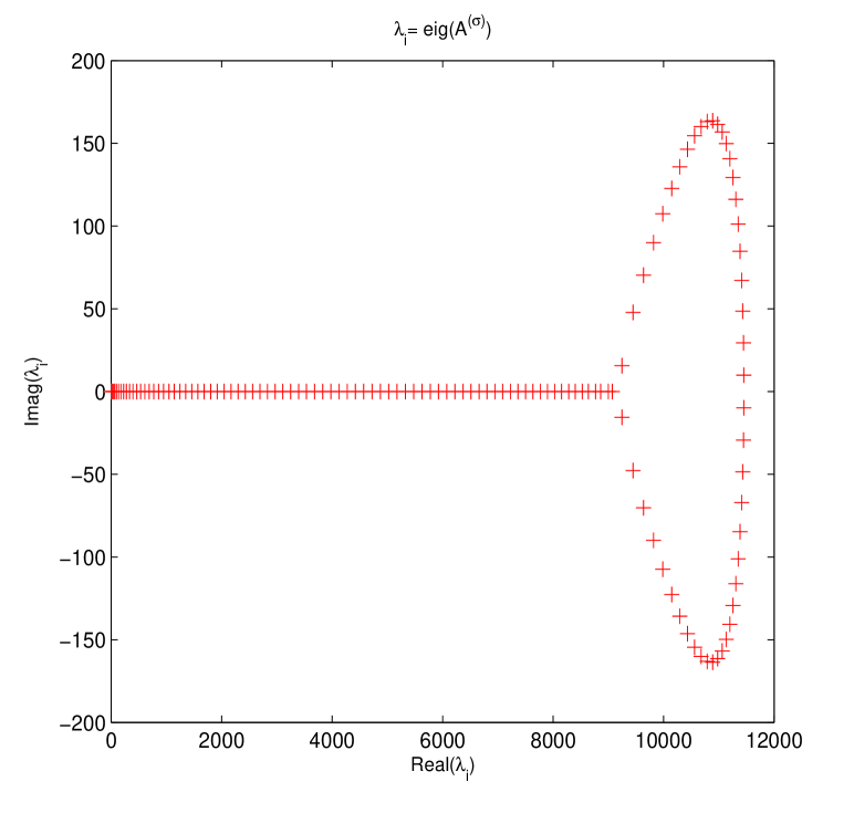
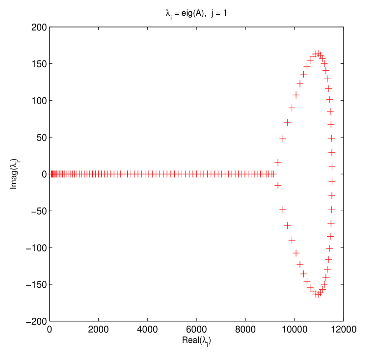
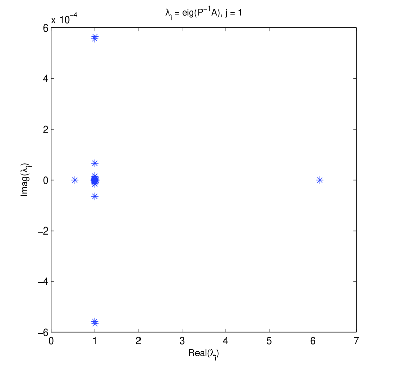
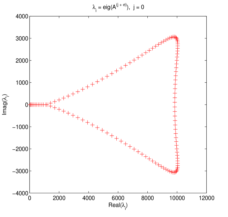
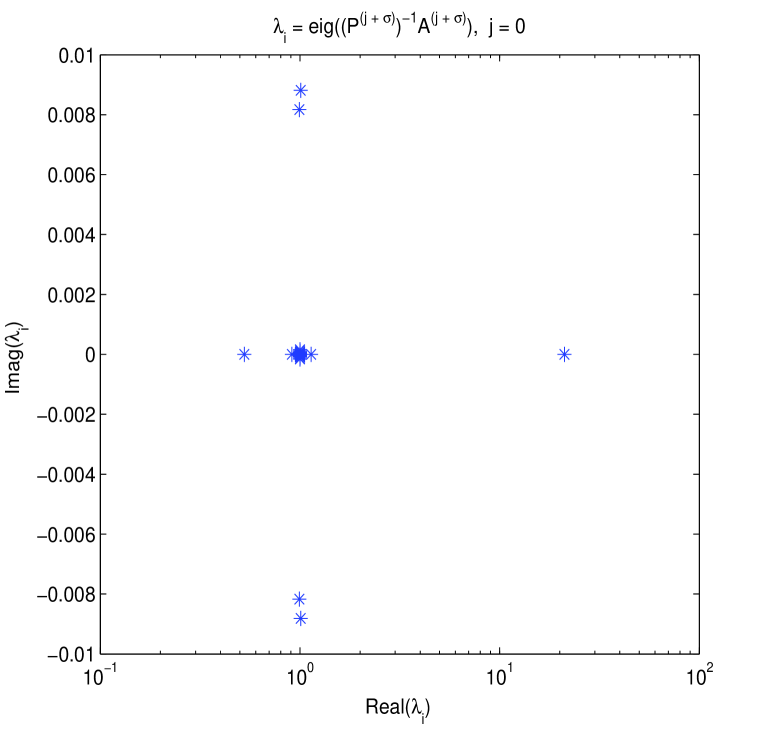
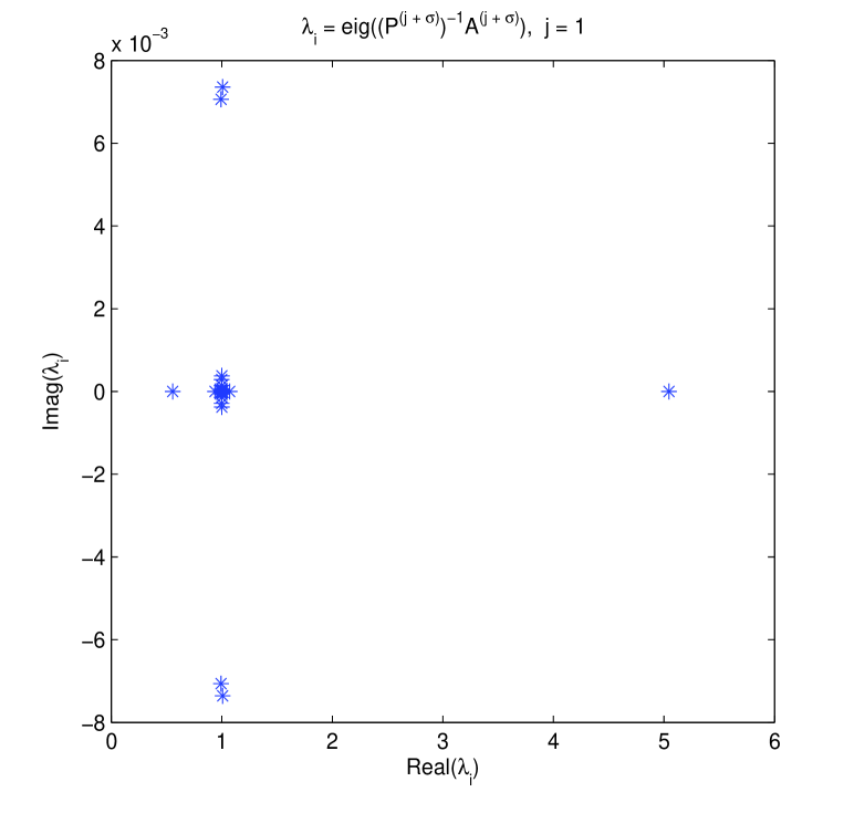
Firstly, some eigenvalue plots about both original and preconditioned matrices are drawn in Figs. 1-2. These two figures confirm that for circulant preconditioning, the eigenvalues of preconditioned matrices are clustered at 1, expect for few (about $6\sim 10$ ) outliers. The vast majority of the eigenvalues are well separated away from 0. It may be interpreted as that in our implementation the number of iterations required by preconditioned Krylov subspace methods almost ranges from 6 to 10. We validate the effectiveness and robustness of the designed circulant preconditioner from the perspective of clustering spectrum distribution.

Table 3: CPU time in seconds for solving Example 1 with

\alpha=0.9

that Time1 is done by for Algorithm 3 (LU decomposition) and Time2 is done by Algorithm 3 with Algorithm 1.

$h=\tau$	Time1	Time2	Speed-up	Time1	Time2	Speed-up	Time1	Time2	Speed-up
	$\beta=1.2$			$\beta=1.5$			$\beta=1.8$
$2^{-5}$	0.003	0.009	0.33	0.003	0.009	0.33	0.003	0.009	0.33
$2^{-6}$	0.011	0.017	0.65	0.011	0.017	0.65	0.011	0.016	0.69
$2^{-7}$	0.061	0.059	1.03	0.062	0.058	1.05	0.062	0.058	1.05
$2^{-8}$	0.344	0.266	1.29	0.336	0.267	1.26	0.335	0.268	1.25
$2^{-9}$	4.319	1.902	2.27	4.317	1.901	2.27	4.338	1.899	2.28
$2^{-10}$	41.683	17.035	2.43	42.106	17.556	2.40	41.808	17.166	2.43

Table 4: CPU time in seconds for solving Example 1 with

\beta=1.8

that Time1 is done by for Algorithm 3 (LU decomposition) and Time2 is done by Algorithm 3 with Algorithm 1.

$h=\tau$	Time1	Time2	Speed-up	Time1	Time2	Speed-up	Time1	Time2	Speed-up
	$\alpha=0.1$			$\alpha=0.5$			$\alpha=0.9$
$2^{-5}$	0.003	0.010	0.30	0.003	0.010	0.30	0.003	0.010	0.30
$2^{-6}$	0.011	0.017	0.65	0.011	0.017	0.65	0.011	0.017	0.65
$2^{-7}$	0.061	0.059	1.03	0.060	0.059	1.02	0.060	0.058	1.03
$2^{-8}$	0.343	0.268	1.28	0.345	0.268	1.29	0.340	0.266	1.28
$2^{-9}$	4.329	1.903	2.27	4.349	1.907	2.28	4.357	1.900	2.27
$2^{-10}$	41.639	17.058	2.44	41.677	17.097	2.44	41.662	16.986	2.45

In Tables 3-4, it illustrates that the proposed fast direct solver for different discretized problems takes much less CPU time elapsed as $M$ and $N$ become large. When $M=N=2^{10}$ and different discretized parameters, the CPU time of Algorithm 3 is about 17 seconds, the speedup is more than 2 times. Meanwhile, although Time1 required by Algorithm 3 for small test problems ( $M=N=32,64$ ) than Time2 needed by Algorithm 3, our proposed method is still more attractive in terms of lower memory requirement. Compared to Algorithm 3 with reusing LU decomposition, it highlighted that in the whole implementation the proposed solution technique does not require to store the full matrices (e.g. some matrices $A^{(\sigma)},A$ and their LU factors) at all. In short, we can conclude that our proposed IDS with fast implementation is still more competitive than the IDS with reusing the conventional LU decomposition.

Example 2. In the last test, we investigate the equation (1.1) on the space interval $[a,b]=[0,1]$ and the time interval $[0,T]=[0,1]$ with diffusion coefficients $d_{+}(t)=9\sin(t),~d_{-}(t)=4\sin(t)$ , convection coefficient $\gamma(t)=-t$ , initial condition $u(x,0)=x^{2}(1-x)^{2}$ , and source term

\begin{split}f(x,t)=&\frac{\Gamma(3+\alpha)}{2}t^{2}x^{2}(1-x)^{2}-(t^{2+\alpha}+1)\Big{\{}-2tx(1-x)(1-2x)+\frac{\Gamma(3)\sin(t)}{\Gamma(3-\beta)}[9x^{2-\beta}\\ &+4(1-x)^{2-\beta}]-\frac{2\Gamma(4)\sin(t)}{\Gamma(4-\beta)}[9x^{3-\beta}+4(1-x)^{3-\beta}]+\frac{\Gamma(5)\sin(t)}{\Gamma(5-\beta)}[9x^{4-\beta}~+\\ &4(1-x)^{4-\beta}]\Big{\}}.\end{split}

The exact solution of this example is defined as $u(x,t)=(t^{2+\alpha})x^{2}(1-x)^{2}$ . For the implicit finite difference discretization, the space step and time step are taken to be $h=1/N$ and $\tau=h$ , respectively. The experiment results about the proposed IDS for Example 3 are reported in Tables 5-6. Furthermore, the effectiveness of fast solution techniques presented in Section 3 for this example will be illustrated in Tables 7-8.

Table 5:

L_{2}

-norm and maximum norm error behavior versus grid size reduction when

\tau=h

and

\beta=1.3

in Example 2.

$\alpha$	$h$	$\max_{0\leq n\leq M}\\|E^{n}\\|_{0}$	CO in $\\|\cdot\\|_{0}$	$\\|E\\|_{\mathcal{C}(\bar{\omega}_{h\tau})}$	CO in $\\|\cdot\\|_{\mathcal{C}(\bar{\omega}_{h\tau})}$
0.10	1/32	3.1941e-4	–	5.6886e-4	–
	1/64	7.6298e-5	2.0657	1.6055e-4	1.8250
	1/128	1.8397e-5	2.0521	4.2694e-5	1.9110
	1/256	4.4694e-5	2.0414	1.1036e-5	1.9519
0.50	1/32	3.0866e-4	–	5.6897e-4	–
	1/64	7.3673e-5	2.0668	1.6054e-4	1.8254
	1/128	1.7757e-5	2.0527	4.2689e-5	1.9110
	1/256	4.3137e-6	2.0414	1.1035e-5	1.9518
0.90	1/32	2.9880e-4	–	5.6951e-4	–
	1/64	7.1478e-5	2.0636	1.6058e-4	1.8264
	1/128	1.7232e-5	2.0524	4.2691e-5	1.9113
	1/256	4.1814e-6	2.0430	1.1034e-5	1.9519
0.99	1/32	3.2304e-4	–	5.7367e-4	–
	1/64	7.7278e-5	2.0638	1.6119e-4	1.8314
	1/128	1.8633e-5	2.0522	4.2748e-5	1.9149
	1/256	4.5227e-6	2.0426	1.1035e-5	1.9538

Table 6:

L_{2}

-norm and maximum norm error behavior versus

\tau

-grid size reduction when

h=1/1200

and

\beta=1.3

in Example 2.

$\alpha$	$\tau$	$\max_{0\leq n\leq M}\\|E^{n}\\|_{0}$	CO in $\\|\cdot\\|_{0}$	$\\|E\\|_{\mathcal{C}(\bar{\omega}_{h\tau})}$	CO in $\\|\cdot\\|_{\mathcal{C}(\bar{\omega}_{h\tau})}$
0.10	1/10	2.0652e-5	–	3.2538e-5	–
	1/20	5.0679e-6	2.0269	7.9617e-6	2.0310
	1/40	1.1568e-6	2.1312	1.7951e-6	2.1490
0.50	1/10	1.3380e-4	–	2.1072e-4	–
	1/20	3.3465e-5	1.9994	5.2683e-5	1.9999
	1/40	8.2623e-6	2.0180	1.2988e-5	2.0202
0.90	1/10	2.6237e-4	–	4.1300e-4	–
	1/20	6.5529e-5	2.0014	1.0313e-4	2.0016
	1/40	1.6266e-5	2.0103	2.5583e-5	2.0112
0.99	1/10	2.8754e-4	–	4.5251e-4	–
	1/20	7.1771e-5	2.0023	1.1293e-4	2.0025
	1/40	1.7825e-5	2.0095	2.8027e-5	2.0105

According to the numerical results illustrated in Table 5, it finds that as the number of the spatial subintervals and time steps is increased keeping $h=\tau$ , a reduction in the maximum error takes place, as expected and the convergence order of the approximate scheme is $\mathcal{O}(h^{2})=\mathcal{O}(\tau^{2})$ , where the convergence order is given by the formula: CO = $\log_{h_{1}/h_{2}}\frac{\|E_{1}\|}{\|E_{2}\|}$ ( $E_{i}$ is the error corresponding to $h_{i}$ ). On the other hand, Table 6 illustrates that if $h=1/1000$ , then as the number of time steps of our approximate scheme is increased, a reduction in the maximum error takes place, as expected and the convergence order of time is $\mathcal{O}(\tau^{2})$ , where the convergence order is given by the following formula: CO = $\log_{\tau_{1}/\tau_{2}}\frac{\|E_{1}\|}{\|E_{2}\|}$ .

Again, for the case of variable time coefficients, several eigenvalue plots about both original and preconditioned matrices are similarly displayed in Figs. 3-4. These two figures confirm that for circulant preconditioning, the eigenvalues of preconditioned matrices are clustered at 1, expect for few (about $6\sim 10$ ) outliers. The vast majority of the eigenvalues are well separated away from 0. It may be mainly interpreted as that in our implementation the number of iterations needed by PCGS with circulant preconditioners almost ranges from 6 to 10. We validate the effectiveness and robustness of the proposed circulant preconditioner from the perspective of clustering spectrum.

Table 7: CPU time in seconds for solving Example 2 with

\alpha=0.9

that Time1 is done by for Algorithm 2 (MATLAB’s backslash) and Time2 is done by Algorithm 2 with PCGS solver.

$h=\tau$	Time1	Time2	Speed-up	Time1	Time2	Speed-up	Time1	Time2	Speed-up
	$\beta=1.3$			$\beta=1.5$			$\beta=1.9$
$2^{-5}$	0.03	0.06	0.50	0.03	0.06	0.50	0.03	0.06	0.50
$2^{-6}$	0.09	0.13	0.69	0.09	0.14	0.64	0.09	0.13	0.69
$2^{-7}$	0.46	0.32	1.44	0.47	0.34	1.38	0.45	0.34	1.32
$2^{-8}$	2.65	0.86	3.08	2.61	0.91	2.87	2.59	0.88	2.94
$2^{-9}$	31.39	3.70	8.48	31.63	3.93	8.05	31.33	3.74	8.38
$2^{-10}$	316.34	22.39	14.13	321.05	22.96	13.98	329.89	22.74	14.51

Table 8: CPU time in seconds for solving Example 2 with

\beta=1.8

that Time1 is done by for Algorithm 2 (MATLAB’s backslash) and Time2 is done by Algorithm 2 with PCGS solver.

$h=\tau$	Time1	Time2	Speed-up	Time1	Time2	Speed-up	Time1	Time2	Speed-up
	$\alpha=0.5$			$\alpha=0.9$			$\alpha=0.99$
$2^{-5}$	0.03	0.06	0.50	0.03	0.06	0.50	0.03	0.06	0.50
$2^{-6}$	0.09	0.13	0.69	0.09	0.13	0.69	0.09	0.13	0.69
$2^{-7}$	0.45	0.35	1.28	0.46	0.34	1.35	0.45	0.34	1.32
$2^{-8}$	2.54	0.98	2.59	2.55	0.89	2.87	2.57	0.90	2.86
$2^{-9}$	31.56	4.14	7.62	31.53	3.92	8.04	31.87	3.88	8.21
$2^{-10}$	328.59	23.46	14.01	328.73	23.15	14.20	329.37	22.83	14.41

In Tables 7-8, it verifies that the proposed fast direct solver for different discretized problems takes much less CPU time elapsed as $M$ and $N$ become large. When $M=N=2^{10}$ and different discretized parameters, the CPU time of Algorithm 3 by PCGS with circulant preconditioners is about 23 seconds, the speedup is almost 14 times. Meanwhile, although Time1 required by Algorithm 3 with MATLAB’s backslash for small test problems ( $M=N=32,64$ ) than Time2 needed by Algorithm 3 with using the PCGS method, our proposed method is still more attractive in aspects of lower memory requirement. Compared to Algorithm 3 with MATLAB’s backslash, it highlighted that in the whole procedure the proposed solution technique does not require to store a series of full matrices (e.g. coefficient matrices $A^{(j+\sigma)},~j=0,1,\ldots,M-1$ ) at all. All in all, we can conclude that our proposed IDS with fast solution techniques is still more promising than the IDS with common implementation.

5 Conclusions

In this paper, the stability and convergence of an implicit difference schemes approximating the time-space fractional convection-diffusion equation of a general form is studied. Sufficient conditions for the unconditional stability of such difference schemes are obtained. For proving the stability of a wide class of difference schemes approximating the time fractional diffusion equation, it is simple enough to check the stability conditions obtained in this paper. Meanwhile, the new difference schemes of the second approximation order in space and the second approximation order in time for the TSFCDE with variable coefficients (in terms of $t$ ) are constructed as well. The stability and convergence of these implicit schemes in the mesh $L_{2}$ -norm with the rate equal to the order of the approximation error are proved. The method can be easily adopted to other TSFCDEs with other boundary conditions. Numerical tests completely confirming the obtained theoretical results are carried out.

More significantly, with the aid of (3.1), we can ameliorate the calculation skill by the implementation of reliable preconditioning iterative techniques, with only computational cost and memory of $\mathcal{O}(N\log N)$ and $\mathcal{O}(N)$ , respectively. Extensive numerical results are reported to illustrate that the efficiency of the proposed preconditioning methods. In future work, we will focus on the extension of the proposed IDS for handling two/three-dimensional TSFCDEs with fast solution techniques subject to various boundary value conditions. Meanwhile, we will also focus on the development of other efficient preconditioners for accelerating the convergence of Krylov subspace solver for the discretized Toeplitz systems; refer, e.g., to our recent work [59] for this topic.

Acknowledgement

We are grateful to Prof. Zhi-Zhong Sun and Dr. Zhao-Peng Hao for their insightful discussions about the convergence analysis of the proposed implicit difference scheme. The work of the first two authors is supported by 973 Program (2013CB329404), NSFC (61370147, 11301057, and 61402082), the Fundamental Research Funds for the Central Universities (ZYGX2013J106, ZYGX2013Z005, and ZYGX2014J084). The work of the last author has been partially implemented with the financial support of the Russian Presidential grant for young scientists MK-3360.2015.1.

References

[1] I. Podlubny, Fractional Differential Equations, vol. 198 of Mathematics in Science and Engineering, Academic Press, Inc., San Diego, CA, 1999.
[2] S.G. Samko, A.A. Kilbas, O.I. Marichev, Fractional Integrals and Derivatives: Theory and Applications, Gordon and Breach Science Publishers, Yverdonn, 1993.
[3] A.A. Kilbas, H.M. Srivastava, J.J. Trujillo, Theory and Applications of Fractional Differential Equations, Elsevier, Amsterdam, 2006.
[4] R. Metzler, J. Klafter, The random walk’s guide to anomalous diffusion: a fractional dynamics approach, Phys. Rep., 339 (2000), pp. 1-77.
[5] A.I. Saichev, G.M. Zaslavsky, Fractional kinetic equations: solutions and applications, Chaos, 7 (1997), pp. 753-764. Available online at http://dx.doi.org/10.1063/1.166272.
[6] Y. Povstenko, Space-time-fractional advection diffusion equation in a plane, in Advances in Modelling and Control of Non-integer-Order Systems, K.J. Latawiec, M. Łukaniszyn, R. Stanisławski eds., Volume 320 of the series Lecture Notes in Electrical Engineering, Springer, 2015, pp. 275-284.
[7] D.A. Benson, S.W. Wheatcraft, M.M. Meerschaert, Application of a fractional advection-dispersion equation, Water Resour. Res., 36 (2000), pp. 1403-1412.
[8] Y.Z. Povstenko, Fundamental solutions to time-fractional advection diffusion equation in a case of two space variables, Math. Probl. Eng., 2014 (2014), Article ID 705364, 7 pages. Available online at http://dx.doi.org/10.1155/2014/705364.
[9] M.M. Meerschaert, C. Tadjeran, Finite difference approximations for fractional advection-dispersion flow equations, J. Comput. Appl. Math., 172 (2004), pp. 65-77.
[10] L. Su, W. Wang, Q. Xu, Finite difference methods for fractional dispersion equations, Appl. Math. Comput., 216 (2010), pp. 3329-3334.
[11] L. Su, W. Wang, Z. Yang, Finite difference approximations for the fractional advection-diffusion equation, Phys. Lett. A, 373 (2009), pp. 4405-4408.
[12] E. Sousa, Finite difference approximations for a fractional advection diffusion problem, J. Comput. Phys., 228 (2009), pp. 4038-4054.
[13] L. Su, W. Wang, H. Wang, A characteristic difference method for the transient fractional convection-diffusion equations, Appl. Numer. Math., 61 (2011), pp. 946-960.
[14] K. Wang, H. Wang, A fast characteristic finite difference method for fractional advection-diffusion equations, Adv. Water Resour., 34 (2011), pp. 810-816.
[15] Z. Deng, V. Singh, L. Bengtsson, Numerical solution of fractional advection-dispersion equation, J. Hydraul. Eng., 130 (2004), pp. 422-431.
[16] Z. Ding, A. Xiao, M. Li, Weighted finite difference methods for a class of space fractional partial differential equations with variable coefficients, J. Comput. Appl. Math., 233 (2010), pp. 1905-1914.
[17] F. Liu, P. Zhuang, K. Burrage, Numerical methods and analysis for a class of fractional advection-dispersion models, Comput. Math. Appl., 64 (2012), pp. 2990-3007.
[18] S. Momani, A.A. Rqayiq, D. Baleanu, A nonstandard finite difference scheme for two-sided space-fractional partial differential equations, Int. J. Bifurcat. Chaos, 22 (2012), 1250079, 5 pages. Available online at http://dx.doi.org/10.1142/S0218127412500794.
[19] M. Chen, W. Deng, A second-order numerical method for two-dimensional two-sided space fractional convection diffusion equation, Appl. Math. Model., 38 (2014), pp. 3244-3259.
[20] W. Deng, M. Chen, Efficient numerical algorithms for three-dimensional fractional partial differential equations, J. Comp. Math., 32 (2014), pp. 371-391.
[21] W. Qu, S.-L. Lei, S.-W. Vong, Circulant and skew-circulant splitting iteration for fractional advection-diffusion equations, Int. J. Comput. Math., 91 (2014), pp. 2232-2242.
[22] N.J. Ford, K. Pal, Y. Yan, An algorithm for the numerical solution of two-sided space-fractional partial differential equations, Comput. Methods Appl. Math., 15 (2015), pp. 497-514.
[23] A.H. Bhrawy, D. Baleanu, A spectral Legendre-Gauss-Lobatto collocation method for a space-fractional advection diffusion equations with variable coefficients, Rep. Math. Phys., 72 (2013), pp. 219-233.
[24] A.H. Bhrawy, M.A. Zaky, A method based on the Jacobi tau approximation for solving multi-term time-space fractional partial differential equations, J. Comput. Phys., 281 (2015), pp. 876-895.
[25] H. Hejazi, T. Moroney, F. Liu, Stability and convergence of a finite volume method for the space fractional advection-dispersion equation, J. Comput. Appl. Math., 255 (2014), pp. 684-697.
[26] W.Y. Tian, W. Deng, Y. Wu, Polynomial spectral collocation method for space fractional advection-diffusion equation, Numerical Methods for Partial Differential Equations, 30 (2014), pp. 514-535.
[27] Y. Lin, C. Xu, Finite difference/spectral approximations for the time-fractional diffusion equation, J. Comput. Phys., 225 (2007), pp. 1533-1552.
[28] M. Cui, A high-order compact exponential scheme for the fractional convection-diffusion equation, J. Comput. Appl. Math., 255 (2014), pp. 404-416.
[29] M. Cui, Compact exponential scheme for the time fractional convection-diffusion reaction equation with variable coefficients, J. Comput. Phys., 280 (2015), pp. 143-163.
[30] A. Mohebbi, M. Abbaszadeh, Compact finite difference scheme for the solution of time fractional advection-dispersion equation, Numer. Algorithms, 63 (2013), pp. 431-452.
[31] S. Momani, An algorithm for solving the fractional convection-diffusion equation with nonlinear source term, Commun. Nonlinear Sci. Numer. Simul., 12 (2007), pp. 1283-1290.
[32] Z. Wang, S. Vong, A high-order exponential ADI scheme for two dimensional time fractional convection-diffusion equations, Comput. Math. Appl., 68 (2014), pp. 185-196.
[33] Z.-J. Fu, W. Chen, H.-T. Yang, Boundary particle method for Laplace transformed time fractional diffusion equations, J. Comput. Phys., 235 (2013), pp. 52-66.
[34] S. Zhai, X. Feng, Y. He, An unconditionally stable compact ADI method for three-dimensional time-fractional convection-diffusion equation, J. Comput. Phys., 269 (2014), pp. 138-155.
[35] P. Zhuang, Y.T. Gu, F. Liu, I. Turner, P.K.D.V. Yarlagadda, Time-dependent fractional advection-diffusion equations by an implicit MLS meshless method, Int. J. Numer. Meth. Eng., 88 (2011), pp. 1346-1362.
[36] Y.-M. Wang, A compact finite difference method for solving a class of time fractional convection-subdiffusion equations, BIT, 55 (2015), pp. 1187-1217.
[37] Y. Zhang, A finite difference method for fractional partial differential equation, Appl. Math. Comput., 215 (2009), pp. 524-529.
[38] Y. Zhang, Finite difference approximations for space-time fractional partial differential equation, J. Numer. Math., 17 (2009), pp. 319-326.
[39] Y. Shao, W. Ma, Finite difference approximations for the two-side space-time fractional advection-diffusion equations, J. Comput. Anal. Appl., 21 (2016), pp. 369-379.
[40] P. Qin, X. Zhang, A numerical method for the space-time fractional convection-diffusion equation, Math. Numer. Sin., 30 (2008), pp. 305-310. (in Chinese)
[41] F. Liu, P. Zhuang, V. Anh, I. Turner, K. Burrage, Stability and convergence of the difference methods for the space-time fractional advection-diffusion equation, Appl. Math. Comput., 191 (2007), pp. 12-20.
[42] Z. Zhao, X.-Q. Jin, M.M. Lin, Preconditioned iterative methods for space-time fractional advection-diffusion equations, J. Comput. Phys., 319 (2016), pp. 266-279.
[43] S. Shen, F. Liu, V. Anh, Numerical approximations and solution techniques for the space-time Riesz-Caputo fractional advection-diffusion equation, Numer. Algorithms, 56 (2011), pp. 383-403.
[44] M. Parvizi, M.R. Eslahchi, M. Dehghan, Numerical solution of fractional advection-diffusion equation with a nonlinear source term, Numer. Algorithms, 68 (2015), pp. 601-629.
[45] Y. Chen, Y. Wu, Y. Cui, Z. Wang, D. Jin, Wavelet method for a class of fractional convection-diffusion equation with variable coefficients, J. Comput. Sci., 1 (2010), pp. 146-149.
[46] S. Irandoust-pakchin, M. Dehghan, S. Abdi-mazraeh, M. Lakestani, Numerical solution for a class of fractional convection-diffusion equations using the flatlet oblique multiwavelets, J. Vib. Control, 20 (2014), pp. 913-924.
[47] A.H. Bhrawy, M.A. Zaky, J.A. Tenreiro Machado, Efficient Legendre spectral tau algorithm for solving the two-sided space-time Caputo fractional advection-dispersion equation, J. Vib. Control, 22 (2016), pp. 2053-2068.
[48] H. Hejazi, T. Moroney, F. Liu, A finite volume method for solving the two-sided time-space fractional advection-dispersion equation, Cent. Eur. J. Phys., 11 (2013), pp. 1275-1283.
[49] W. Jiang, Y. Lin, Approximate solution of the fractional advection-dispersion equation, Comput. Phys. Commun., 181 (2010), pp. 557-561.
[50] J. Wei, Y. Chen, B. Li, M. Yi, Numerical solution of space-time fractional convection-diffusion equations with variable coefficients using Haar wavelets, Comput. Model. Eng. Sci. (CMES), 89 (2012), pp. 481-495.
[51] M. Ng, Iterative Methods for Toeplitz Systems, Oxford University Press, New York, 2004.
[52] F.-R. Lin, S.-W. Yang, X.-Q. Jin, Preconditioned iterative methods for fractional diffusion equation, J. Comput. Phys., 256 (2014), pp. 109-117.
[53] S.-L. Lei, H.-W. Sun, A circulant preconditioner for fractional diffusion equations, J. Comput. Phys., 242 (2013), pp. 715-725.
[54] I. Gohberg, A. Semencul, On the inversion of finite Toeplitz matrices and their continuous analogues, Matem. Issled., 7 (1972), pp. 201-223. (in Russian)
[55] Y. Saad, Iterative Methods for Sparse Linear Systems, 2nd edition, SIAM, Philadelphia, USA, 2003.
[56] A.A. Alikhanov, A new difference scheme for the time fractional diffusion equation, J. Comput. Phys., 280 (2015), pp. 424-438.
[57] Z.-P. Hao, Z.-Z. Sun, W.-R. Cao, A fourth-order approximation of fractional derivatives with its applications, J. Comput. Phys., 281 (2015), pp. 787-805.
[58] S. Vong, P. Lyu, X. Chen, S.-L. Lei, High order finite difference method for time-space fractional differential equations with Caputo and Riemann-Liouville derivatives, Numer. Algorithms, 72 (2016), pp. 195-210.
[59] X.-M. Gu, T.-Z. Huang, H.-B. Li, L. Li, W.-H. Luo, On $k$ -step CSCS-based polynomial preconditioners for Toeplitz linear systems with application to fractional diffusion equations, Appl. Math. Lett., 42 (2015), pp. 53-58.
[60] Å. Björck, Direct Methods for Linear Systems, in Numerical Methods in Matrix Computations, Volume 59 of the series Texts in Applied Mathematics, Springer, Switzerland, 2014, pp. 1-209.