Fast magnetic wave could heat the solar low-beta chromosphere
Abstract
Magnetohydrodynamic (MHD) waves are candidates for heating the solar chromosphere, although it is still unclear which mode of the wave is dominant in heating. We perform two-dimensional radiative MHD simulation to investigate the propagation of MHD waves in the quiet region of the solar chromosphere. We identify the mode of the shock waves by using the relationship between gas pressure and magnetic pressure across the shock front and calculate their corresponding heating rate through the entropy jump to obtain a quantitative understanding of the wave heating process in the chromosphere. Our result shows that the fast magnetic wave is significant in heating the low-beta chromosphere. The low-beta fast magnetic waves are generated from high-beta fast acoustic waves via mode conversion crossing the equipartition layer. Efficient mode conversion is achieved by large attacking angles between the propagation direction of the shock waves and the chromospheric magnetic field.
1 Introduction
Mechanical heating is required to maintain the energy balance in the solar chromosphere, as suggested by the temperature difference between the radiative equilibrium atmospheric model (Anderson & Athay, 1989) and the observation-based semi-empirical model (Vernazza et al., 1981). Waves have been recognized as important contributors to chromospheric heating, although their heating mechanisms are elusive (see Jess et al., 2015, for a review). While the propagation of waves in the chromosphere has been well studied from both the observational and theoretical perspectives (e.g., Bogdan et al., 2003; Hasan & Ulmschneider, 2004; Hasan et al., 2005; Hasan & van Ballegooijen, 2008; Vigeesh et al., 2009; Heggland et al., 2011; Vigeesh et al., 2012; de la Cruz Rodríguez et al., 2013; Kontogiannis et al., 2016; Santamaria et al., 2016; Kayshap et al., 2018; Abbasvand et al., 2020), a firm quantitative conclusion is still a distance away.
In the chromosphere, physical parameters change drastically, leading to difficulties in studying chromospheric dynamics. The plasma beta varies in both the vertical and horizontal directions, and waves can change their modes when crossing the equipartition layer (Cally, 2006; Pennicott & Cally, 2019) where the speed of sound is identical to the Alfvén speed. Density stratification also adds to the complexity by increasing the amplitude of the acoustic waves, leading to increased nonlinearity and formation of shocks.
In the high-beta regions of the chromosphere where the role of the magnetic field could be ignored, the propagation of acoustic waves has been well studied by hydrodynamic simulations with non-local thermodynamic equilibrium (non-LTE) radiative transfer (Carlsson & Stein, 1995, 1997). In these studies, waves are generated by longitudinal piston motion. They succeed in reproducing the Ca II spectral profile which agrees with the observations.
The situation becomes even more complicated in the low-beta chromosphere with the participation of the magnetic field. Arber et al. (2016) and Brady & Arber (2016) show that the shock heating rate in the chromosphere is larger than or consistent with the observation-based radiative cooling rate. A similar result is also obtained in Wang & Yokoyama (2020) with an improved treatment of the radiative loss term introduced by Carlsson & Leenaarts (2012). In Arber et al. (2016), Brady & Arber (2016), and Wang & Yokoyama (2020), waves are generated by artificial transverse torque or transverse motion at the bottom of the flux tube. These studies do not include the effect of waves originating from outside the flux tube.
Theoretical studies could be divided into two categories, idealized models and realistic models. Arber et al. (2016), Brady & Arber (2016), and Wang & Yokoyama (2020) are examples of idealized models. The physical process is clear in idealized models, but the results are affected by artificial settings in the model. On the other hand, there are also realistic models (e.g., Kato et al., 2011; Carlsson et al., 2016; Iijima & Yokoyama, 2017; Martínez-Sykora et al., 2017) that aim to include complicated physical processes to approach reality. Realistic models are used to reproduce the synthesized images or spectral profiles for comparison with observations (e.g., Leenaarts et al., 2013, 2009; Quintero Noda et al., 2019), but their complexity makes it difficult to understand the underlying elemental physical processes involved in heating. These studies do not focus on the physical processes that occur during wave propagation such as thermalization, nonlinear steepening, or mode conversions in the chromosphere.
The purpose of our study is to conduct a quantitative investigation on wave heating in the chromosphere. In particular, previous studies do not focus on the role of the fast magnetic wave in heating the low-beta chromosphere. We perform a realistic two-dimensional radiative MHD simulation while conducting a detailed investigation on the propagation of waves to estimate the contribution to chromospheric heating by different modes of waves. To achieve this goal, we develop a novel method of automatically identifying the mode of waves and calculating the heating rate due to different modes of waves.
2 Numerical model
We use RAMENS code (Iijima, 2016; Iijima & Yokoyama, 2015) which solves MHD equations with gravity, heat conduction, equation of state under local thermodynamic equilibrium (LTE) condition, radiative transfer in the photosphere, and approximated radiative loss term in the chromosphere and the corona. The basic equations of the simulation are the same as those in Iijima & Yokoyama (2017). One could refer to Iijima (2016) for a detailed description of this code. We modified the original RAMENS code by replacing the treatment of the chromospheric radiative loss term with the improved recipe developed by Carlsson & Leenaarts (2012).
The simulation domain is a 16 Mm 16 Mm two-dimensional square extending from 2 Mm below the photosphere to 14 Mm in the corona with a uniform grid spacing of 8.5 km. The temperature of the corona is 1 MK which is maintained by the top boundary condition. The initial magnetic field is vertical and has a strength of 6 G. We start with a plane parallel atmosphere in the hydrostatic equilibrium state, though this setup does not strongly influence the later results obtained after the well-developed magneto-convections. The data analyzed cover 1000 s of the simulation which is approximately 10 times the transit time for acoustic waves in the chromosphere.
3 Shock identification and heating rate calculation
Our study focuses on wave heating in the low-beta chromosphere. Comparing this mechanism with other possible heating mechanisms (e.g., reconnection and turbulence with ambipolar diffusion), there is observational evidence showing that waves can carry enough energy for chromospheric heating (Bello González et al., 2010). Waves are generated by photospheric convection and steepen to shocks as they propagate upward in the chromosphere. To estimate the shock-heating rate, we identify the shock front in the chromosphere, determine the mode of each shock, and calculate the corresponding heating rate. The positions of the shock fronts are identified by the local minimum of with
| (1) |
where is a parameter indicating the threshold for identification, is the speed of sound, and is the grid size. The value of the parameter should depend on the shock-capturing quality of the numerical scheme and was taken to be in this study (see Appendix in Wang & Yokoyama, 2020).
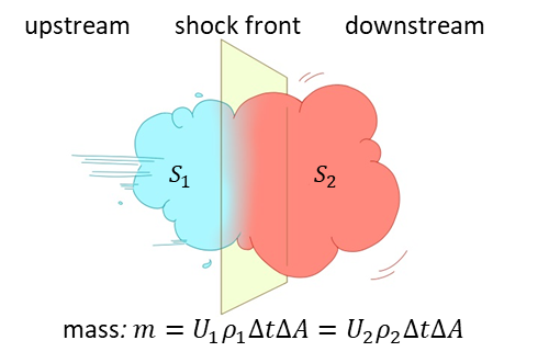
The heating rate at the shock front is calculated using the following steps. First, we extract the density, temperature, velocity, gas pressure, and magnetic pressure along the direction of propagation which is assumed to be identical to the direction of the gradient of the total pressure. The upstream and downstream quantities of the detected shock are determined as the first local maximum and minimum of beside where is the velocity along the direction of propagation, is the distance along the direction of propagation, and is the position of the shock front. The upstream side is determined by the side with the lower density. We estimate the increment of the thermal energy flux at the shock front:
| (2) |
where is the increase in the thermal energy flux. Subscripts 1 and 2 denote the physical parameters that are sampled at the upstream and downstream region, respectively. is the shock-normal velocity in the shock rest frame, is the temperature, and is the entropy per unit mass. is calculated by mass conservation, , and the velocity relationship in different frames of reference, where is the density and is the shock-normal velocity in the laboratory frame (see Figure 1 for a schematic plot). To estimate the heating rate per unit volume, we assume that the heating is evenly distributed in the volume of one grid point at the shock front. As a result, the heating rate per unit volume is calculated by
| (3) |
where is the width of the shock wave. Although the actual thickness in the real shocks should be given by the microscopic dissipation process, we here use the grid spacing for convenience. The heating rate is calculated each time step. We assume that the heating rate at a fixed position do not change within one time step. Note that the spatially integrated amount of is independent of the choice of and is used only for the later discussion.
Finally, we determine the mode of each shock wave by checking whether the gas pressure and the magnetic pressure across the shock front change in the same direction. The sign of across the shock front is used to determine whether it is a fast shock (positive value) or slow shock (negative value), where is the gas pressure and is the magnetic pressure. We do not use phase speed to determine the mode of waves since it is difficult to obtain the local fast speed and slow speed in the dynamic chromosphere.
4 Results
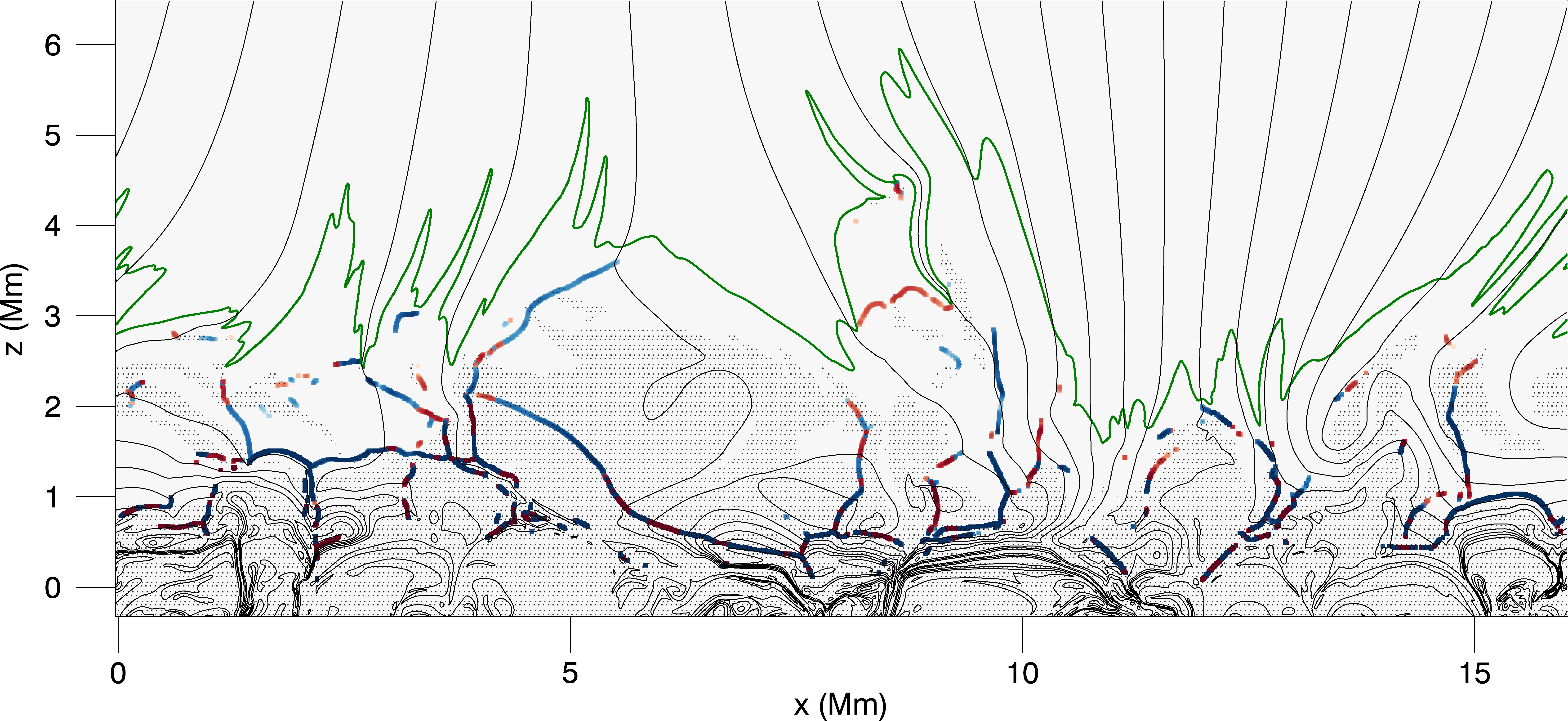
Figure 2 shows the identified shock fronts in the dynamic simulation of solar chromosphere. Waves are generated by photospheric convection and they steepen to shocks in the chromosphere. Shocks dissipate their energy continuously in the chromosphere. A number of shocks gradually become undetectable during their propagation due to dissipation. When shocks impinge on the transition region, they drive the upward motion of the transition region that forms spicules.
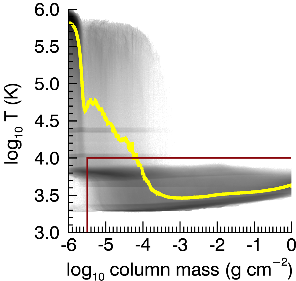
We focus on the low-beta chromospheric plasma. Due to the large deformation of the transition region by the spicules, we cannot distinguish the chromosphere and the corona using a simple threshold on the geometrical height. The low-beta chromospheric plasma is defined by the following criteria: (1) , (2) K, and (3) Alfvén speed is larger than sound speed. The variable is the column mass, and , where is the height of the top of the simulation box. The temperature and column mass threshold are used to exclude coronal plasma. The values of the thresholds are chosen from the joint probability density distribution of the temperature and the column mass (Figure 3).
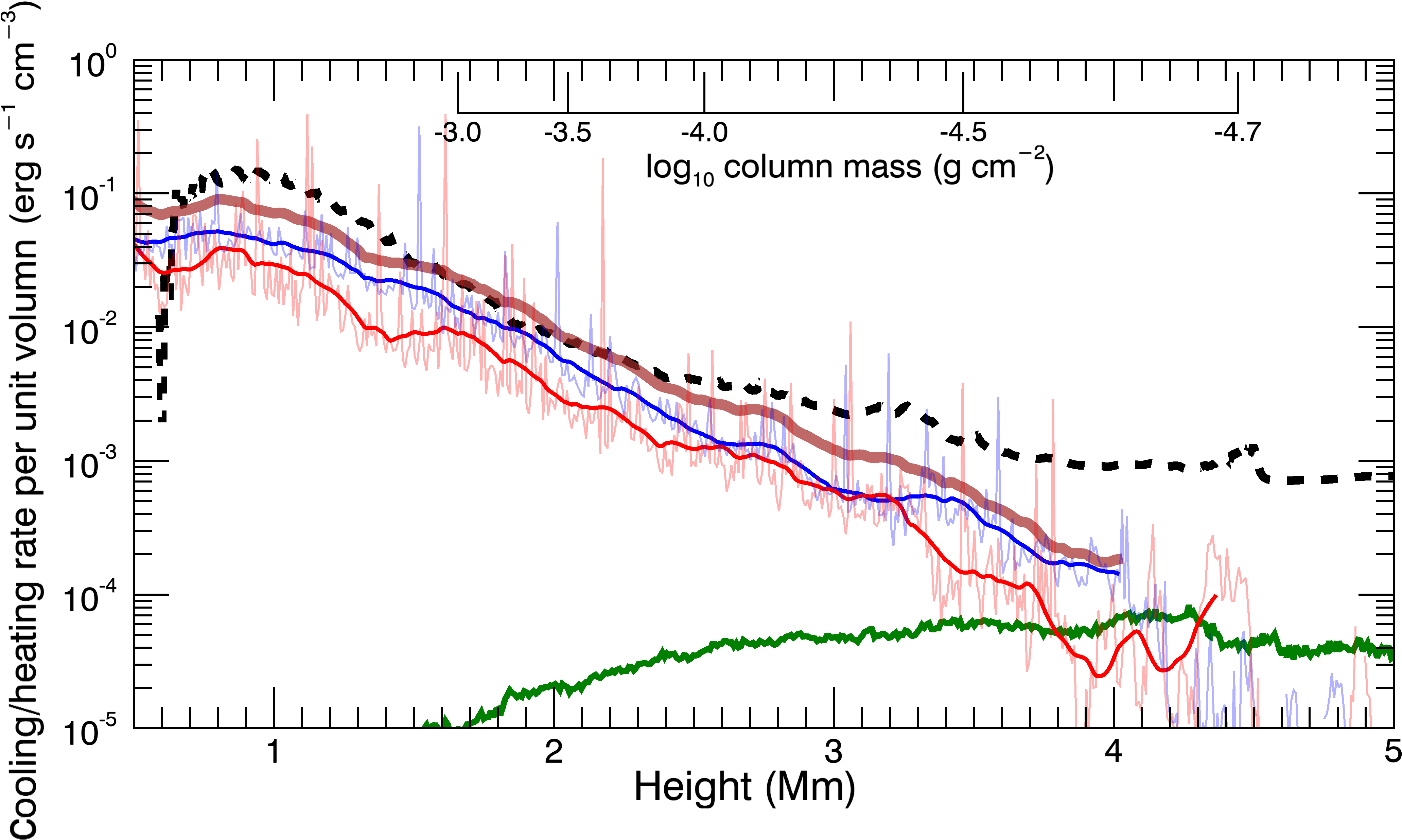
The time and horizontal averaged radiative loss rate and heating rate of the low-beta chromospheric plasma are shown in Figure 4. It is shown that the shock heating is well balanced with radiative cooling below 2.5 Mm. At locations higher than 2.5 Mm, the energy balance is gradually disrupted due to the formation of spicules (in the presence of spicules, the energy balance at a fixed position is determined by the entropy flow carried by them).
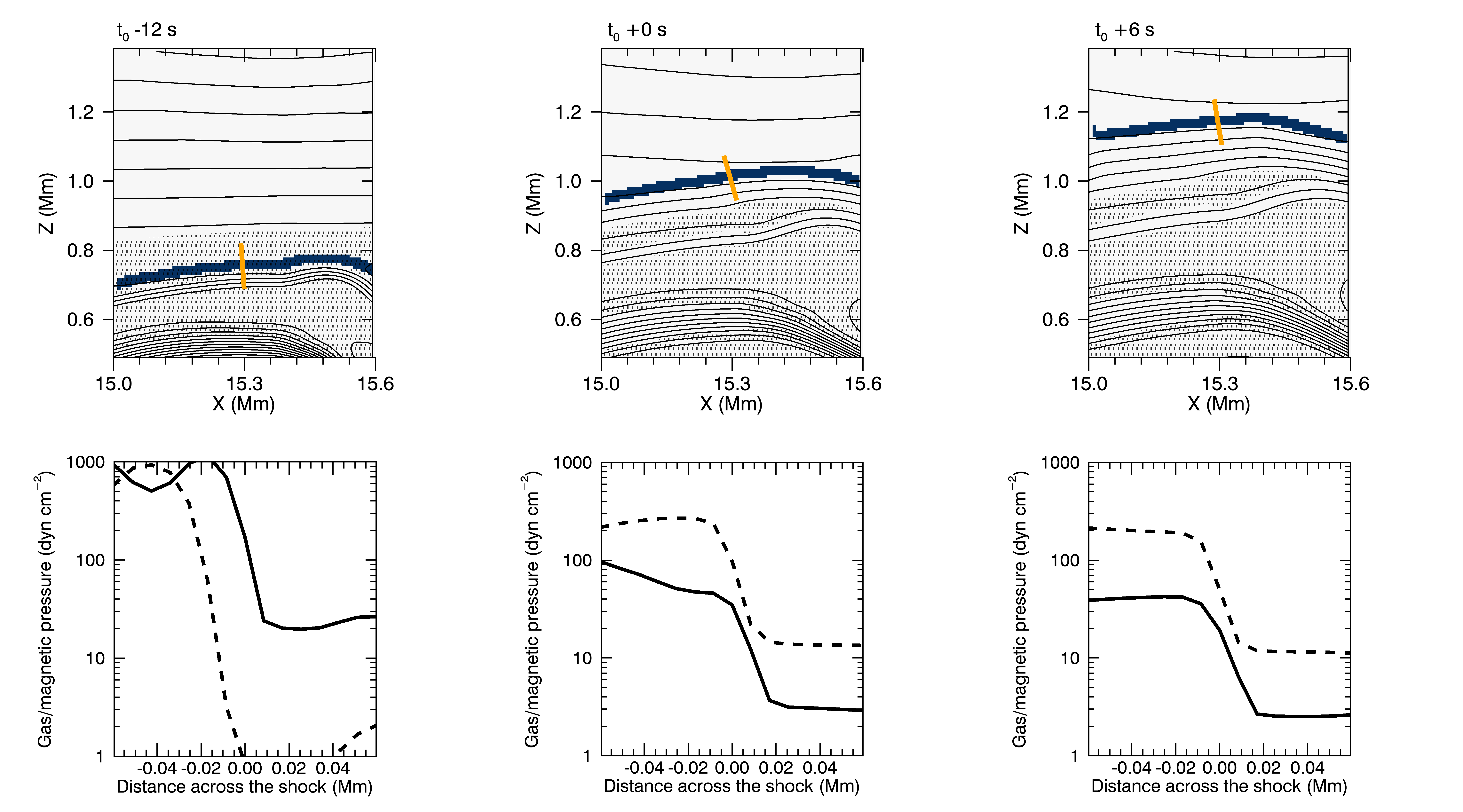
Where do these fast mode waves in the low-beta regions originate? We find that low-beta fast magnetic waves originate from high-beta fast acoustic waves through mode conversion. An example of mode conversion is shown in Figure 5. Mode conversion occurs when fast acoustic waves propagate from the high-beta region to the low-beta region and cross the equipartition layer. An attacking angle (the angle between the wavevector and the magnetic field) close to will result in a larger conversion rate (Cally, 2006; Pennicott & Cally, 2019).
5 Discussion
The propagation of waves in MHD simulation with an idealized setting is also carried on in previous researches (Hasan et al., 2005; Hasan & van Ballegooijen, 2008; Vigeesh et al., 2009, 2012). These studies mainly focus on waves that originate inside a flux tube. For these waves, as they propagate upwards, they propagate along the magnetic field lines thus the attacking angle is small and mode conversion is less efficient. Hasan & van Ballegooijen (2008) do mention the waves that originate outside a flux tube could generate fast magnetic waves in the flux tube through mode conversion but they do not discuss the heating by the fast magnetic waves in detail. Our result shows that, with quantification of the heating rate, fast waves do play a role in heating the low-beta chromosphere.
Khomenko & Collados (2006) show that refraction could affect the propagation of fast waves and prevent their efficient energy transport to the chromosphere. They focus on waves inside a strong flux tube (sunspots). On the other hand, in our simulation, fast waves in the regions between two flux tubes are less affected by refraction since there is no substantial horizontal gradient of fast speed in these regions. In addition, the intensity of magnetic field in the flux tube is weaker in our simulation which also reduces the horizontal gradient of fast speed.
Our simulation shows that shock heating is the dominant heating process in the chromosphere. This result is consistent with those from previous studies. However, the wave modes contributing to heating are different. In Arber et al. (2016), Wang & Yokoyama (2020) and Hasan & Ulmschneider (2004), transverse waves at the foot of a low-beta flux tube undergo nonlinear mode coupling and generate slow acoustic waves. They steepen to shocks which dissipate and contribute to chromospheric heating. In our simulation, Alfvèn waves vanish because of the two-dimensional geometry. As a result, the nonlinear mode coupling is also absent.
As fast waves propagate like an expanding sphere, the strongest perturbation of the vertical velocity appears at the top of the sphere, whereas compression of the vertical magnetic field appears at the lateral sides. In our simulation, the background magnetic field is 6 G, mimicking the quiet sun region. The resultant intensity of the magnetic field perturbation in the chromosphere could be as large as 10–20 G. The combination of vertical velocity and vertical magnetic field perturbation can be used as a signal of the fast wave. Such a signal can hopefully be detected by next-generation solar telescopes such as Daniel K. Inouye Solar Telescope (DKIST; Rimmele et al., 2020) and Chinese Giant Solar Telescope (CGST; Deng & CGST Group, 2011).
In order to investigate effect of the topology of magnetic field line, we carry on another simulation with the same initial and boundary condition described in Section 2. The only difference is that we increase the intensity of the initial background magnetic field from 6 G to 20 G. In this new setting, the magnetic field lines are less inclined which results in smaller attacking angle for waves that propagate upward. We find that the percentage of heating by slow wave increases, especially in the higher part of the chromosphere characterized by . However, our main result that fast magnetic shock waves play a significant role in heating the low-beta chromosphere remains unchanged.
Our study is limited in the quiet region. In sunspots, observations show that wave energy is insufficient for chromospheric heating (Felipe et al., 2011). In these regions, other effects related with magnetic field such as reconnection should be taken into consideration.
In this study, the ambipolar diffusion and dynamic ionization of hydrogen are not considered. The dissipation of ambipolar diffusion could lead to substantial heating locally (Khomenko & Collados, 2012; Shelyag et al., 2016; Martínez-Sykora et al., 2017; Soler et al., 2019). On the other hand, Arber et al. (2016) compare the time-averaged heating rate resulting from ambipolar diffusion and shock dissipation and find that shock heating is much stronger than the heating resulting from ambipolar diffusion. Leenaarts et al. (2007) compare simulations with the LTE assumption and dynamic ionization. It is shown that in the simulation with dynamic ionization, shock temperatures are higher and the intershock temperatures are lower than in the simulation with the LTE assumption. This effect could affect the measurement of the entropy jump. Moreover, dynamic ionization is important to determine the electron and the ion number density and will further affect the estimation of ambipolar diffusion, especially when the ionization degree is low. Further studies that compare shock heating, turbulence heating (van Ballegooijen et al., 2011), and ambipolar diffusion (Leake et al., 2005; Khomenko et al., 2018; Martínez-Sykora et al., 2020; González-Morales et al., 2020) in realistic simulations are expected to be conducted in the future.
6 Conclusion
We perform a two-dimensional MHD simulation to study the propagation of MHD waves in the chromosphere. We identify the mode of the shock waves in the chromosphere, calculate the heating rate from the entropy jump, and find that the heating rate balances with the radiative loss. Fast magnetic shock waves play a significant role in heating the low-beta chromosphere. These low-beta fast magnetic waves are generated by mode conversion.
We acknowledge the referee for valuable comments. The authors thank M. Carlsson for providing numerical tables for the recipe of the chromospheric radiative loss. The authors thank B. Yu’s assistance in making Figure 1. Numerical computations were carried out on Cray XC50 at Center for Computational Astrophysics, National Astronomical Observatory of Japan. T.Y. is supported by JSPS KAKENHI grant No. 15H03640, No. 20KK0072, and No. 21H01124. H.I. is supported by JSPS KAKENHI grant No. 19K14756.
References
- Abbasvand et al. (2020) Abbasvand, V., Sobotka, M., Heinzel, P., Švanda, M., Jurčák, J., del Moro, D., & Berrilli, F. 2020, ApJ, 890, 22
- Anderson & Athay (1989) Anderson, L. S., & Athay, R. G. 1989, ApJ, 346, 1010
- Arber et al. (2016) Arber, T. D., Brady, C. S., & Shelyag, S. 2016, ApJ, 817, 94
- Bello González et al. (2010) Bello González, N., et al. 2010, ApJL, 723, L134
- Bogdan et al. (2003) Bogdan, T. J., et al. 2003, ApJ, 599, 626
- Brady & Arber (2016) Brady, C. S., & Arber, T. D. 2016, ApJ, 829, 80
- Cally (2006) Cally, P. S. 2006, Philosophical Transactions of the Royal Society of London Series A, 364, 333
- Carlsson et al. (2016) Carlsson, M., Hansteen, V. H., Gudiksen, B. V., Leenaarts, J., & De Pontieu, B. 2016, A&A, 585, A4
- Carlsson & Leenaarts (2012) Carlsson, M., & Leenaarts, J. 2012, A&A, 539, A39
- Carlsson & Stein (1995) Carlsson, M., & Stein, R. F. 1995, ApJ, 440, L29
- Carlsson & Stein (1997) —. 1997, ApJ, 481, 500
- de la Cruz Rodríguez et al. (2013) de la Cruz Rodríguez, J., De Pontieu, B., Carlsson, M., & Rouppe van der Voort, L. H. M. 2013, ApJ, 764, L11
- Deng & CGST Group (2011) Deng, Y. Y., & CGST Group. 2011, in Astronomical Society of India Conference Series, Vol. 2, Astronomical Society of India Conference Series, 31–36
- Felipe et al. (2011) Felipe, T., Khomenko, E., & Collados, M. 2011, ApJ, 735, 65
- González-Morales et al. (2020) González-Morales, P. A., Khomenko, E., Vitas, N., & Collados, M. 2020, A&A, 642, A220
- Hasan & Ulmschneider (2004) Hasan, S. S., & Ulmschneider, P. 2004, A&A, 422, 1085
- Hasan & van Ballegooijen (2008) Hasan, S. S., & van Ballegooijen, A. A. 2008, ApJ, 680, 1542
- Hasan et al. (2005) Hasan, S. S., van Ballegooijen, A. A., Kalkofen, W., & Steiner, O. 2005, ApJ, 631, 1270
- Heggland et al. (2011) Heggland, L., Hansteen, V. H., De Pontieu, B., & Carlsson, M. 2011, ApJ, 743, 142
- Iijima (2016) Iijima, H. 2016, PhD thesis, Department of Earth and Planetary Science, School of Science, The University of Tokyo, Japan
- Iijima & Yokoyama (2015) Iijima, H., & Yokoyama, T. 2015, ApJ, 812, L30
- Iijima & Yokoyama (2017) —. 2017, ApJ, 848, 38
- Jess et al. (2015) Jess, D. B., Morton, R. J., Verth, G., Fedun, V., Grant, S. D. T., & Giagkiozis, I. 2015, SSRev, 190, 103
- Kato et al. (2011) Kato, Y., Steiner, O., Steffen, M., & Suematsu, Y. 2011, ApJ, 730, L24
- Kayshap et al. (2018) Kayshap, P., Murawski, K., Srivastava, A. K., Musielak, Z. E., & Dwivedi, B. N. 2018, MNRAS, 479, 5512
- Khomenko & Collados (2006) Khomenko, E., & Collados, M. 2006, ApJ, 653, 739
- Khomenko & Collados (2012) —. 2012, ApJ, 747, 87
- Khomenko et al. (2018) Khomenko, E., Vitas, N., Collados, M., & de Vicente, A. 2018, A&A, 618, A87
- Kontogiannis et al. (2016) Kontogiannis, I., Tsiropoula, G., & Tziotziou, K. 2016, A&A, 585, A110
- Leake et al. (2005) Leake, J. E., Arber, T. D., & Khodachenko, M. L. 2005, A&A, 442, 1091
- Leenaarts et al. (2009) Leenaarts, J., Carlsson, M., Hansteen, V., & Rouppe van der Voort, L. 2009, ApJ, 694, L128
- Leenaarts et al. (2007) Leenaarts, J., Carlsson, M., Hansteen, V., & Rutten, R. J. 2007, A&A, 473, 625
- Leenaarts et al. (2013) Leenaarts, J., Pereira, T. M. D., Carlsson, M., Uitenbroek, H., & De Pontieu, B. 2013, ApJ, 772, 90
- Martínez-Sykora et al. (2017) Martínez-Sykora, J., De Pontieu, B., Hansteen, V. H., Rouppe van der Voort, L., Carlsson, M., & Pereira, T. M. D. 2017, Science, 356, 1269
- Martínez-Sykora et al. (2020) Martínez-Sykora, J., Leenaarts, J., De Pontieu, B., Nóbrega-Siverio, D., Hansteen, V. H., Carlsson, M., & Szydlarski, M. 2020, ApJ, 889, 95
- Pennicott & Cally (2019) Pennicott, J. D., & Cally, P. S. 2019, ApJ, 881, L21
- Quintero Noda et al. (2019) Quintero Noda, C., et al. 2019, MNRAS, 486, 4203
- Rimmele et al. (2020) Rimmele, T. R., et al. 2020, Sol. Phys., 295, 172
- Santamaria et al. (2016) Santamaria, I. C., Khomenko, E., Collados, M., & de Vicente, A. 2016, A&A, 590, L3
- Shelyag et al. (2016) Shelyag, S., Khomenko, E., de Vicente, A., & Przybylski, D. 2016, ApJ, 819, L11
- Soler et al. (2019) Soler, R., Terradas, J., Oliver, R., & Ballester, J. L. 2019, ApJ, 871, 3
- van Ballegooijen et al. (2011) van Ballegooijen, A. A., Asgari-Targhi, M., Cranmer, S. R., & DeLuca, E. E. 2011, ApJ, 736, 3
- Vernazza et al. (1981) Vernazza, J. E., Avrett, E. H., & Loeser, R. 1981, ApJS, 45, 635
- Vigeesh et al. (2012) Vigeesh, G., Fedun, V., Hasan, S. S., & Erdélyi, R. 2012, ApJ, 755, 18
- Vigeesh et al. (2009) Vigeesh, G., Hasan, S. S., & Steiner, O. 2009, A&A, 508, 951
- Wang & Yokoyama (2020) Wang, Y., & Yokoyama, T. 2020, ApJ, 891, 110