Fast Non-Adiabatic Dynamics of Many-Body Quantum Systems

Modeling many-body quantum systems with strong interactions is one of the core challenges of modern physics. A range of methods has been developed to approach this task, each with its own idiosyncrasies, approximations, and realm of applicabilityMotta2017 . Perhaps the most successful and ubiquitous of these approaches is density functional theory (DFT)Hohenberg1964 . Its Kohn-Sham formulation Kohn1965 has been the basis for many fundamental physical insights, and it has been successfully applied to fields as diverse as quantum chemistry, condensed matter and dense plasmas White2013 ; Witte2017 ; Dharma-wardana2006 ; Bauernschmitt1996 ; Burke2012 ; Ziegler1991 ; Jones2015 . Despite the progress made by DFT and related schemes, however, there remain many problems that are intractable for existing methods. In particular, many approaches face a huge computational barrier when modeling large numbers of coupled electrons and ions at finite temperature Baczewski2016 ; Jones2015 ; Mabey2017 . Here, we address this shortfall with a new approach to modeling many-body quantum systems. Based on the Bohmian trajectories formalism Bohm1952 ; Bohm1953 , our new method treats the full particle dynamics with a considerable increase in computational speed. As a result, we are able to perform large-scale simulations of coupled electron-ion systems without employing the adiabatic Born-Oppenheimer approximation.

Let us consider a many-particle electron-ion system at finite temperature. In calculating the dynamics of both the electrons and ions, we must account for the fact that the ions evolve multiple orders of magnitude more slowly than the electrons, as a result of their much higher masses. If we are interested in the long-time ionic dynamics (for example, the ion mode structure), we face a choice of how to deal with this timescale issue. We can either model the system on the time scale of the electrons – non-adiabatically – and incur a significant computational cost (a cost that is prohibitive in most simulation schemes); or we can model the system on the timescale of the ions – adiabatically – by treating the electrons as a static, instantaneously adjusting background. The latter approach is far cheaper computationally, but does not allow for a viable description of the interplay of ion and electron dynamics.

The method we propose here enables us to employ the former (non-adiabatic) approach, retaining the dynamic coupling between electrons and ions, by significantly reducing the simulation’s computational demands. We achieve this by treating the system dynamics with linearized Bohmian trajectories. Having numerical properties similar to those of molecular dynamics for classical particles, our approach permits calculations previously out of reach: systems containing thousands of particles can be modeled for long (ionic) time periods, so that dynamic ion modes can be calculated without discounting electron dynamics.

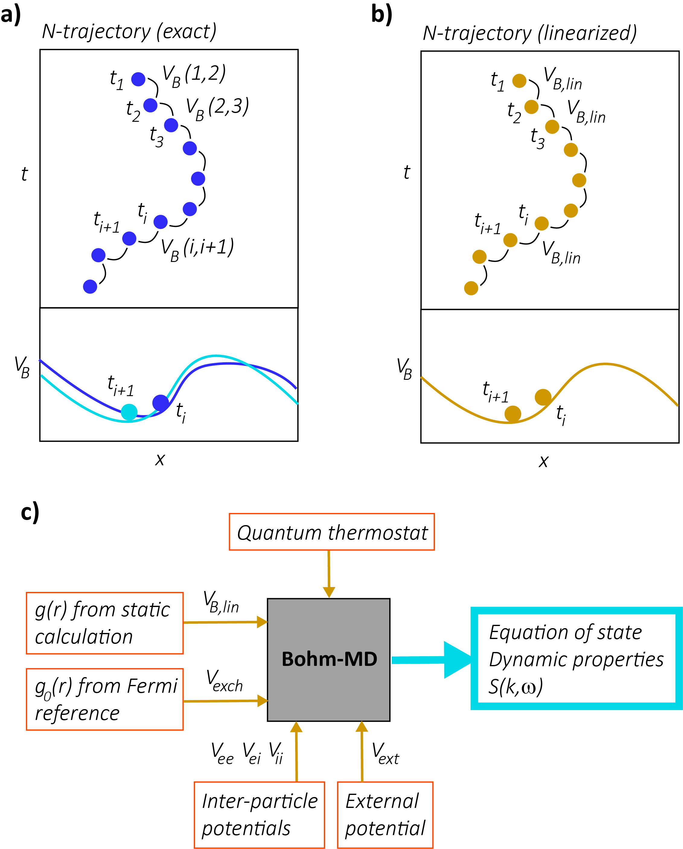
To begin constructing our method, we consider Bohm’s formulation of quantum mechanics. We can imagine a classical $N$-body system as a “$N$-trajectory” moving through 3$N$-dimensional configuration space. Bohm’s theory treats an $N$-body quantum system as an ensemble of these classical $N$-trajectories, interacting through an additional $N$-body potential $V_{B}$. This Bohm potential is a functional of the density of $N$-trajectories in configuration space, $\Phi$, and a function of the spatial position ${\bf x}$; that is, $V_{B}=V_{B}({\bf x}|\Phi)$. Provided matching initial conditions, the Bohm ensemble of $N$-trajectories reproduces the dynamics of the probability density – as given by the Schrödinger equation – exactly Bohm1952 (see also Supplementary Information for more details).

In its exact form, Bohm’s formulation is as intractable as the $N$-body Schrödinger equation, requiring simulation of a huge number of $N$-body interacting classical systems. However, we can construct a fast computational method solving Bohm’s theory by introducing a thermally averaged, linearized Bohm potential. The exact (but inaccessible) calculation for a pure quantum state with many particles – based on the theory above – would require us to propagate an array of $N$-trajectories through time, at each step recalculating their density and thereby $V_{B}$ (see Fig. 1a). Reliable calculations of density in $3N$-dimensional space would require a prohibitive number of $N$-trajectories, however, making this unfeasible. Here, we propose an alternative: as opposed to applying this theory to a pure quantum state, we consider propagating an array of thermally coupled $N$-trajectories in a similar manner, as a model of a system at finite temperature. Our core assumption is that the time evolution of a finite-temperature quantum system can be approximated by a similar procedure to that used for the pure state; we consider an array of $N$-trajectories, each coupled to a heat bath setting its temperature, evolving under a potential that is a functional of $N$-trajectory density in configuration space. This procedure can be seen as a trajectory-based analogue of the linearization of the Bohm potential over states in quantum hydrodynamics Manfredi2005 .

For simplicity, we focus initially on systems in thermal equilibrium. We allow our thermal $N$-trajectories – together modeling the probability density of our finite-temperature system – to evolve in time under a linearized mean Bohm potential of the underlying pure states. In this linear approximation, we replace the mean Bohm potential experienced, expressible as a sum over functionals of individual states, with a functional of a sum over individual states.

In addition to moving focus from a pure state to a more practically important finite-temperature state, the key feature of our approximation is that it dramatically reduces the computational expense required to simulate the system (as compared to the exact pure state case). Crucially, now that we are considering finite-temperature $N$-trajectories, we need only track a single $N$-trajectory through time, rather than an impractical number of them. This follows from two observations:

1. Properties of a classical system with correlation-dependent potentials can be determined self-consistently. For an arbitrary system of $N$ well-localized particles, the $N$-particle correlation function can be written as $g({\bf x})=P({\bf x})/P_{0}({\bf x})$, where $P$ denotes the joint positional probability distribution of the particles, and $P_{0}$ is the distribution for a non-interacting classical system with equal particle densities. Here, the variable ${\bf x}$ is the set of particle positions, ${\bf x}=\{{\bf x}_{1},{\bf x}_{2},...,{\bf x}_{N}\}$. We may construct inter-particle potentials that are functionals of $g$: $V({\bf x})=V_{0}({\bf x})+V_{g}({\bf x}|g)$, where $V_{0}$ denotes pair interactions and external forces, and $V_{g}$ is a contribution that varies with $g$. The equilibrium properties of a system in this potential can be found self-consistently. Starting from an initial guess for $V({\bf x})$, we can calculate $g({\bf x})$, through a Monte Carlo simulation or a similar method Allen2017 . This value of the $N$-particle correlation function $g$ then gives rise to a new approximation for the potential. Iterating this procedure allows for both $g$ and $V$ to be found.

2. Our linearized Bohmian system is equivalent to a classical system with correlation-dependent potentials. Consider a number of coupled thermal $N$-trajectories representing our linearized Bohmian system. Assuming that the system is in a temperature regime in which the particle motion is ergodic, we find that each $N$-trajectory has the same time-integrated correlations; that is, each has the same $g$. In the limit of infinite $N$-trajectories in our ensemble, it follows that the configuration space density of $N$-trajectories $\Phi$ is exactly proportional to this common $g$. As a result, each $N$-trajectory moves in a common static potential (see Fig. 1b), and, as this static potential is a functional of configuration space density, $\Phi$, it is equivalently just a functional of $g$.

When combining the results above, our linearization approximation becomes a simple mapping:

where $m_{i}$ is the mass of particle $i$ and $\lambda$ is a linearization factor that still needs to be determined. As $g$ is common to all $N$-trajectories, our approximation scheme allows us to consider just a single $N$-body classical system (Fig. 1b). The required simulation is thus amenable to (computationally cheap) classical Molecular Dynamics Allen2017 . The classical particle trajectories simulated then approximate the statistics of the full quantum system.

Before the scheme above can be implemented, we must overcome a final fundamental hurdle: the full correlation function $g$ appearing in Eq. (1) is too complicated to be modeled directly (similar to the full $N$-body wavefunction). Therefore, we seek an approximate closure for this object in terms of lower-order correlations, which can be calculated accurately. For this goal, we employ the pair product approximation, whereby the $N$-body correlation is replaced by a product of pair correlations. Further, we generalize the dependence on $\lambda$ to a set of $\lambda_{ij}$ to accommodate different particle species in the pair interactions.

We need an additional correction to our potentials to fulfil the spin statistics theorem, as the Schrödinger equation – and thus Bohmian mechanics – does not incorporate particle spin directly. In particular, this correction will generate a Fermi distribution for the electrons in thermal equilibrium. Similar to successful approaches applied in quantum hydrodynamics and classical map methods Manfredi2005 ; Lado1967 ; Dharma-Wardana2012 , we introduce an additional Pauli potential term. This term is constructed such that exchange effects are reproduced exactly for a reference electron gas system. We also employ pseudo-potentials, commonly applied in modern DFT calculations, to represent core electrons bound in deep shells of the ions by an effective ion potential seen by the valence electrons.

Finally, it remains to set the linearization parameters $\lambda_{ij}$ to fully determine the system’s Hamiltonian. In this work, we take $\lambda_{ij}=1$ for the ion-ion and ion-electron terms. To determine the electron-electron parameter $\lambda_{ee}$, we match static ion correlations – that is, pair distribution functions – obtained by DFT calculations. This matching can be carried out rigorously with a generalized form of inverse Monte Carlo (see Supplement Information). In this way, we determine $\lambda_{ee}$ with only static information of the system. Subsequent dynamic simulations can then be carried out without any free parameters.

We can now implement the Bohmian dynamics method with a Molecular Dynamics simulation inclusive of the potentials discussed above. Within the microcanonical ensemble, we could simply integrate the equation of motion for the particles. However, we want to simulate systems with a given temperature which requires the coupling of the system to a heat bath. Here, we employ a modified version of the Nosé-Hoover thermostat. Its standard form is popular in classical Molecular Dynamics studies, achieving reliable thermodynamic properties while having minimal impact on the dynamics Basconi2013 . We use this standard version to control the ion temperature. The electrons, however, should relax to a Fermi distribution, which is not possible with this classical form. We have thus produced a modified version of the Nosé-Hoover thermostat for the dynamic electrons. It creates an equilibrium distribution equal to that of a non-interacting electron gas of the same density (see Supplementary Information for details and derivation). With this, we ensure the ions interact with an electron subsystem with a corrected energy distribution.

To demonstrate the strength of our new method, we apply it to warm dense matter (WDM). With densities comparable to solids and temperatures of a few electron volts, WDM combines the need for quantum simulations of degenerate electrons with the description of a strongly interacting ion component. These requirements make WDM an ideal testbed for quantum simulations. Further, as the matter in the mantle and core of large planets is in a WDM state Guillot1999 ; Kerley1972 , and experiments towards inertial confinement fusion exhibit WDM states transiently on the path to ignition Glenzer2010 ; Hu2015 , simulations of WDM are of crucial importance in modern applications.

Key dynamic properties of the WDM state can be represented by the dynamic structure factor (DSF) Hansen2013 . This quantity also connects theory and experiment: probabilities for diffraction and inelastic scattering are directly proportional to the DSF GarciaSaiz2008 ; Glenzer2009 ; Fletcher2015 , allowing testing of WDM models. Here, we focus on the ion-ion DSF that is defined via

where $N$ is the total number of ions and $\rho({\bf k},t)$ is the spatial Fourier transform of the ion density. In the following, we assume the WDM system to be isotropic and spatially uniform. Accordingly, the structure factor depends only on the magnitude of the wavenumber, $k=|{\bf k}|$. While the main contribution to $S(k,\omega)$ is due to direct Coulomb interactions between the ions, the modifications due to screening are strongly affected by quantum behavior in the electron component.

Recent work has shown that predictions from standard DFT simulations for the ion-ion DSF are problematic due to the use of the Born-Oppenheimer approximation Mabey2017 . Employing a Langevin thermostat, it has been found that the dynamics of the electron-ion interaction may strongly change the mode structure – in particular, the strength of the diffusive mode. However, this approach requires a very simple, uniform frequency dependence for electron-ion collisions, which may not prove realistic in practice. It also contains an arbitrary parameter, the Langevin friction, and is of limited predictive power as a result.

We demonstrate here that our new method of Bohmian dynamics, that retains the dynamics of the electron-ion interaction, can overcome the shortcomings of previous approaches without introducing free parameters. The specific case we consider is compressed liquid aluminum with a density of $5.2$ gcm^-3 and a temperature of $3.5$ eV, which allows for direct comparison with previous results. Full details of the corresponding simulations and input parameters are given in the Supplementary Information.

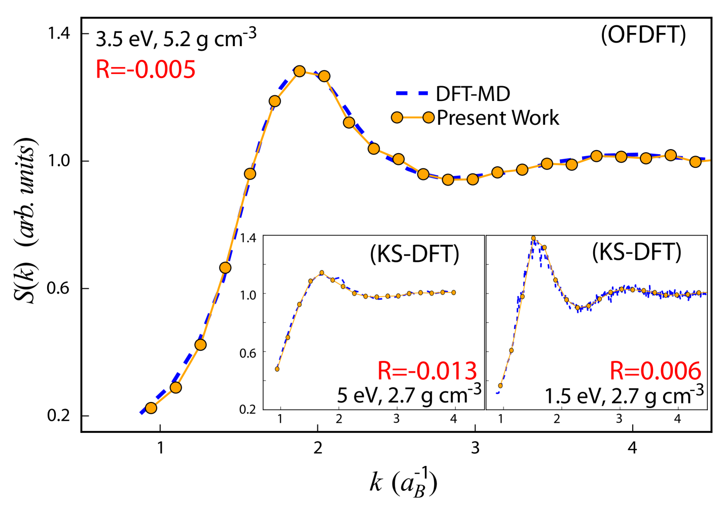
The validity and accuracy of our implementation of Bohmian dynamics is strongly supported by the excellent reproduction of static ion-ion correlations from DFT simulations. Fig. 2 illustrates the static ion-ion structure factor obtained with the Bohmian trajectories technique described above. The comparisons with orbital free DFT and the computationally more intensive Kohn-Sham DFT both yield agreement within the statistical error of the simulations. As discussed, this match was achieved by a single parameter fit defining $\lambda_{ee}$. The different simulation techniques predict almost the same thermodynamics as shown by the small pressure difference.

Fig. 3a shows calculations of the fully frequency-dependent DSF. One can clearly notice the appearance of side peaks in the DSF that correspond to ion acoustic waves. Their dispersion for smaller wavenumbers, and the corresponding sound speed, are very sensitive to the interactions present in the system. Thus, they reflect the screening of ions by electrons as well as dynamic electron-ion collisions. For larger wavenumbers $k$, these modes cease to exist due to increased damping. The data also exhibit a diffusive mode around $\omega=0$ although it is not as prominent as predicted in Ref. Mabey2017 .

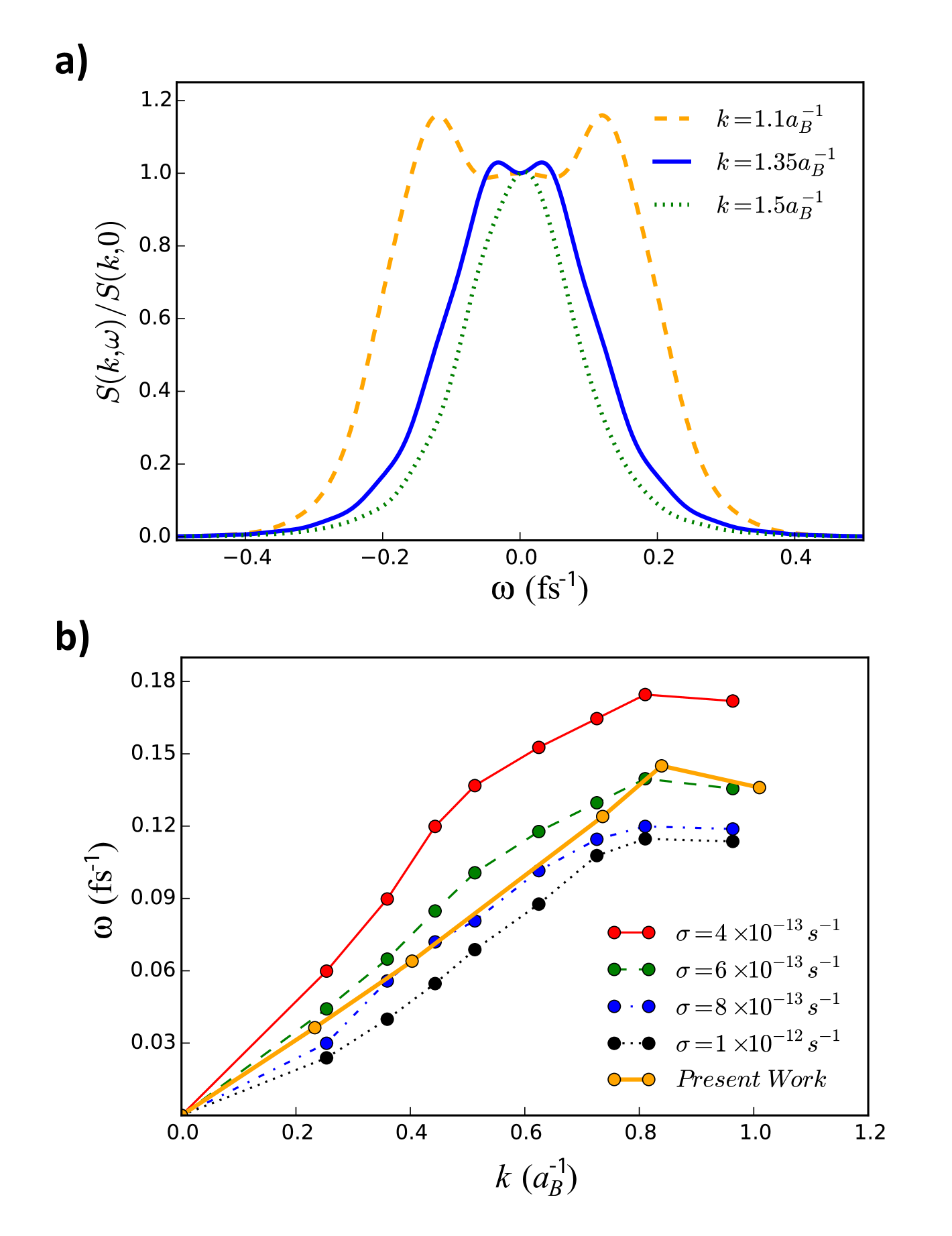
The dispersion relation of the ion acoustic modes is displayed in Fig. 3b, which also contains results from the Langevin approach. The latter approach requires ad hoc friction parameters which were chosen to cover the range between the classical and quantum Born limits (see Ref. Mabey2017 ). The strength of the Bohmian approach lies in the fact that it does not require a free parameter, thereby allowing access to a self-consistent prediction of the sound speed. This comparison may also be used to assess the quality of the friction parameter applied in the Langevin approach. For the case considered, one finds that neither the classical nor the weak coupling Born limit are applicable – a finding which is typical of the WDM regime.

The upper results demonstrate the strength of the Bohmian approach in modeling quantum systems with strong interactions and nonlinear ion dynamics. For static and thermodynamic properties, we obtain results in very close agreement with DFT simulations. In addition, while the standard implementation of DFT involves the Born-Oppenheimer approximation, our Bohm approach can treat electrons and ions non-adiabatically, retaining the full coupling of the electron and ion dynamics. As a result, we can investigate the changes of the ion modes due to dynamic electron-ion correlations which are inaccessible to standard DFT. In contrast to a Langevin model, we have no free parameters and can thus predict the strength of the electron drag to the ion motion. Simulations based on time-dependent DFT Marques2004 represent another way to avoid the Born-Oppenheimer approximation. However, this method is numerically extremely expensive, drastically limiting particle numbers and simulations times; at present, this limitation precludes results for the ion modes as presented here.

The principal advantage of our approach is its relative numerical speed, which allows for the modeling of quantum systems with large numbers of particles. For comparison, the recent time-dependent DFT simulation of Ref. Baczewski2016 models a system of 128 electrons for approximately 0.001 attoseconds per CPU-core and second. The comparative Bohmian dynamics system models 8 times as many electrons for approximately 20 attoseconds per CPU-core and second. This vast difference in computation time enables our method to access a new class of correlated quantum systems. Such calculations are relevant not just for WDM, but also address core problems in time-dependent chemical reactions, biological systems (e.g., protein folding), and radiation damage of materials protein ; poccia ; suga .

References

- [1] Motta, M. et al. Towards the solution of the many-electron problem in real materials: equation of state of the hydrogen chain with state-of-the-art many-body methods. Phys. Rev. X 7, 031059 (2017).
- [2] Hohenberg, P. & Kohn, W. Inhomogeneous electron gas. Phys. Rev. 136, B864 (1964).
- [3] Kohn, W. & Sham, L. J. Self-consistent equations including exchange and correlation effects. Physical Review 140, A1133 (1965).
- [4] White, T. G., Richardson, S., Crowley, B. J. B., Pattison, L. K., Harris, J. W. O. & Gregori,G. Orbital-free density-functional theory simulations of the dynamic structure factor of warm dense aluminum. Phys. Rev. Lett. 111, 175002 (2013).
- [5] Knudson, M.D., Desjarlais, M.P., Becker, A., Lempke, R.W., Cochrane, K.R., Savage, M.E., Bliss, D.E., Mattsson, T.R. & Redmer, R. Direct observation of an abrupt insulator-to-metal transition in dense liquid deuterium. Science 348, 1455 (2015).
- [6] Dharma-Wardana, M. W. C. Static and dynamic conductivity of warm dense matter within a density-functional approach: application to aluminum and gold. Phys. Rev. E 73, 036401 (2006).
- [7] Bauernschmitt, R. & Ahlrichs, R. Treatment of electronic excitations within the adiabatic approximation of time dependent density functional theory. Chem. Phys. Lett. 256, 454 (1996).
- [8] Burke, K. Perspective on density functional theory. J. Chem. Phys. 136, 150901 (2012).
- [9] Ziegler, T. Approximate density functional theory as a practical tool in molecular energetics and dynamics. Chem. Rev. 91, 651 (1991).
- [10] Jones, R. O. Density functional theory: its origins, rise to prominence, and future. Rev. Mod. Phys. 87, 897 (2015).
- [11] Baczewski, A. D., Shulenburger, L., Desjarlais, M. P., Hansen, S. B. & Magyar, R. J. X-ray Thomson scattering in warm dense matter without the Chihara decomposition. Phys. Rev. Lett. 116, 115004 (2016).
- [12] Mabey, P., Richardson, S., White, T. G., Fletcher, L. B., Glenzer, S. H. Hartley, N. J., Vorberger, J., Gericke, D. O. & Gregori, G. A strong diffusive ion mode in dense ionized matter predicted by Langevin dynamics. Nat. Comm. 8, 14125 (2017).
- [13] Bohm, D. A suggested interpretation of the quantum theory in terms of “hidden” variables. I. Phys. Rev. 85, 166 (1952).
- [14] Bohm, D. A collective description of electron interactions: III. Coulomb interactions in a degenerate electron gas. Phys. Rev. 92, 609 (1953).
- [15] Allen, M. P. & Tildesley, D. J. Computer Simulation of Liquids. (Oxford University Press, 2017).
- [16] Manfredi, G. How to model quantum plasmas. arXiv:quant-ph/0505004 (2005).
- [17] Lado, F. Effective potential description of the quantum ideal gases. J. Chem. Phys. 47, 5369 (1967).
- [18] Dharma-Wardana, M. W. C. The classical-map hyper-netted-chain (CHNC) method and associated novel density-functional techniques for warm dense matter. Int. J. Quantum Chem. 112, 53 (2012).
- [19] Basconi, J. E. & Shirts, M. R. Effects of temperature control algorithms on transport properties and kinetics in molecular dynamics simulations. J. Chem. Theory and Computation 9, 2887 (2013).
- [20] Guillot, T. Interiors of giant planets inside and outside the solar system. Science 286, 72 (1999).
- [21] Kerley, G. I. Equation of state and phase diagram of dense hydrogen. Phys. Earth and Planetary Interiors 6, 78 (1972).
- [22] Glenzer, S. H. et al. Symmetric inertial confinement fusion implosions at ultra-high laser energies. Science 327, 1228 (2010).
- [23] Hu, S. X., Goncharov, V. N., Boehly, T. R., McCrory, R. L., Skupsky, S., Collins, L. A., Kress, J. D. & Militzer, B. Impact of first-principles properties of deuterium-tritium on inertial confinement fusion target designs. Phys. Plasmas 22, 056304 (2015).
- [24] Hansen, J.P. & McDonald, I. R. Theory of Simple Liquids. (Academic Press, 2013).
- [25] Garcia Saiz, E. et al. Probing warm dense lithium by inelastic X-ray scattering. Nat. Physics 4, 940 (2008).
- [26] Glenzer, S. H. & Redmer, R. X-ray Thomson scattering in high energy density plasmas. Rev. Mod. Phys. 81, 1625 (2009).
- [27] Fletcher, L. B. et al. Ultrabright X-ray laser scattering for dynamic warm dense matter physics. Nat. Photonics 9, 274 (2015).
- [28] Marques, M.A.L. & Gross, E.K.U. Time-dependent density functional theory. Ann. Rev. Phys. Chem. 55, 427 (2004).
- [29] Dill, K.A. & MacCallum, J.L. The Protein-Folding Problem, 50 Years On. Science 338, 1042 (2012).
- [30] Poccia, N., Fratini, M., Ricci, A., Campi, G., Barba, L., Vittorini-Orgeas, A., Bianconi, G., Aeppli, G. & Bianconi, A. Evolution and control of oxygen order in a cuprate superconductor. Nat. Materials 10, 733 (2011).
- [31] Suga, M. et al. Light-induced structural changes and the site of O=O bond formation in PSII caught by XFEL. Nature 543, 131 (2017).