Current address: ]Nord Quantique, Sherbrooke, Québec, J1K 0A5, Canada
Fast parametric two-qubit gates with suppressed residual interaction
using a parity-violated superconducting qubit
Abstract
We demonstrate fast two-qubit gates using a parity-violated superconducting qubit consisting of a capacitively-shunted asymmetric Josephson-junction loop under a finite magnetic flux bias. The second-order nonlinearity manifesting in the qubit enables the interaction with a neighboring single-junction transmon qubit via first-order inter-qubit sideband transitions with Rabi frequencies up to 30 MHz. Simultaneously, the unwanted static longitudinal (ZZ) interaction is eliminated with ac Stark shifts induced by a continuous microwave drive near-resonant to the sideband transitions. The average fidelities of the two-qubit gates are evaluated with randomized benchmarking as 0.967, 0.951, 0.956 for CZ, iSWAP and SWAP gates, respectively.
Quantum information processing with superconducting qubits has been intensively studied recently. High-fidelity quantum manipulations and projective measurements have been achieved in multi-qubit systems martinis2014 ; ibm2016 ; rigetti ; martinis2019 ; johnson2020 , and basic quantum error-correction protocols have been demonstrated schoelkopf2012 ; martinis2015 ; schoelkopf2016 ; correct2019 ; wallraf2019 . For fault-tolerant quantum computing, however, the gate and readout fidelity should be further improved by a few orders of magnitude fowler ; terhal .
To this end, a variety of two-qubit gates have been proposed and demonstrated. These can be classified into two groups, based on their use of either a coupling between (near-)degenerate qubits martinis2014 ; martinis2019 or a microwave-induced parametric coupling nakamura2007 ; ibm2011 ; ibm2016 ; rigetti ; johnson2020 ; screview . For the gate operation, the former usually requires fast frequency tuning of the qubits and/or a coupler through a flux bias, while the latter only uses microwave pulses for the dynamical control. For the parametric gates, qubits are usually far off-resonant from each other in order to suppress residual couplings between them. On the other hand, a large detuning slows down the parametric gate, causing a trade-off that hinders the improvement of the gate fidelity. Recent works have addressed this issue by introducing various types of coupler circuits to eliminate the residual coupling without sacrificing the gate speed significantly DiVincenzo2017 ; steele2018 ; houck2019 ; duan2020 . A simpler scheme combining two qubits with opposite signs of anharmonicity also allows a residual-coupling-free two-qubit cross-resonance gate plourde2020 .
In this letter, we propose and demonstrate fast parametric two-qubit gates using sideband transitions between an ordinary transmon qubit and a parity-violated superconducting qubit, which we call a cubic transmon. The parity violation originates in a cubic component of the inductive potential of a Josephson-junction circuit under a finite magnetic flux bias. This circuit, known as a superconducting nonlinear asymmetric inductive element (SNAIL), was recently proposed SNAIL and utilized in parametric amplifiers SNAIL2 , bosonic-mode qubits SNAIL3 , and hybrid quantum systems noguchi2018 . The parity symmetry breaking is essential for a physical system to acquire a second-order nonlinearity, which allows three-wave-mixing-type first-order sideband transitions and thus the parametric interactions with a neighboring qubit nakamura2015 ; sideband ; DiVincenzo2016 . The large capacitive coupling strength between the qubits introduces strong parametric interactions, but also a large residual static interaction. We eliminate the latter by using ac Stark shifts induced by a continuous near-resonant drive of the sideband transitions and solve the trade-off. This approach of microwave-assisted elimination of the static interactions brings in more tuning knobs, i.e. amplitudes and frequencies of multiple drives, which can be applied to the cases with multiple qubits and higher-order residual couplings.
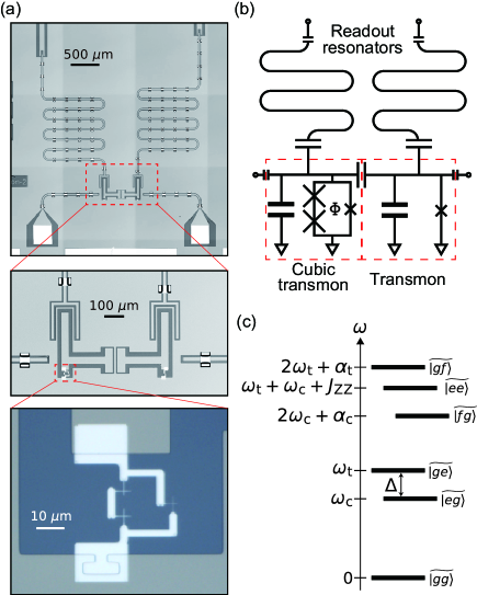
Figures 1(a) and 1(b) present optical micrographs and a circuit diagram of the device, which contains two superconducting qubits and two resonators for the dispersive readout of each qubit. The qubit on the right-hand side is a conventional transmon, which is composed of a capacitively-shunted single Josephson junction koch2007 . The other qubit is a cubic transmon, which is a capacitively-shunted SNAIL circuit. The SNAIL is a Josephson-junction loop formed by a parallel circuit of a single small Josephson-junction and two large Josephson junctions. The SNAIL loop is threaded by a flux . The Hamiltonian of the two-qubit system reads
| (1) | |||||
where is the reduced Planck constant, and are the bare eigenmode frequencies, and and are the annihilation operators for the cubic transmon and conventional transmon, respectively. The coefficient is the second-order nonlinearity of the cubic transmon, and are the third-order nonlinearities of each qubit, and is the capacitive coupling strength between the two qubits.
In the dispersive coupling regime , the effective Hamiltonian can be written as
| (2) | |||||
where () is the effective coupling strength, and , , , and are the eigenmode frequencies and self-Kerr nonlinearities of the qubits after the perturbative treatment of the coupling term in Eq. (1), respectively. The term with a coefficient arises from the second-order nonlinearity in the parity-violated cubic transmon and gives the interaction in the same form as the radiation pressure in optomechanics optomechanics ; noguchi2018 and the state-dependent force in trapped ions blatt2008 ; ion . There is also a static longitudinal (ZZ) interaction between the qubits, whose amplitude is . The detailed derivations and expressions of the parameters in Eqs. (1) and (2) are presented in the Supplementary Material supple .
Figure 1(c) illustrates the eigenstates and their frequencies. The coupling between qubits hybridizes the bare qubit states, , and forms the eigenstates supple . When a drive field at frequency is applied to the cubic transmon, the two qubits resonate with each other in the rotating frame. Under the rotating-wave approximation, the parametric coupling follows
| (3) | |||||
| (4) |
where and are the amplitude and phase of the drive field, respectively. Note that is proportional to the second-order nonlinearity for the three-wave-mixing process occurring under the Hamiltonian in Eq. (3).
Under the resonant condition , the drive exchanges the excitation of the two qubits, and thus the iSWAP and SWAP gates can be implemented. Another type of two-qubit gate, controlled-phase (CZ) gate, is similarly achieved with a parametric drive. When the drive frequency is equal to , the transition takes place. A -rotation of the transition induces a geometric phase factor of only to the state in the computational subspace.
In parallel with the dynamically-induced coupling, there remains the spurious static ZZ interaction, the last term in Eq. (2), between the capacitively coupled qubits with higher energy levels ibm2019 . Remarkably, the residual interaction can be eliminated also with a parametric drive. We irradiate the cubic transmon with a continuous-wave (CW) microwave field, whose frequency is slightly detuned from the transition of . The ac Stark effect by the CW drive shifts the eigenfrequencies in the two-qubit subspace. These shifts give rise to a tunable ZZ interaction and allow compensation for the unwanted interaction.
In the experiment, we use the device shown in Fig. 1. The parameters at the operating flux bias, , where , are the followings: The eigenfrequencies of the cubic transmon and the transmon are and , respectively. The third-order nonlinearities of the qubits are and , and the bare coupling strength between the qubits is , which are determined by spectroscopic measurements. The details of the sample characterization are described in the Supplementary Material supple . Using these values, we estimate the second-order nonlinearity , the effective coupling strength , and the coupling coefficient of the parametric drive, . The energy-relaxation and Ramsey-dephasing times of the qubits are and for the cubic transmon, and and for the transmon, respectively. The dephasing time of the cubic transmon is improved to with an echo pulse, while no change is seen for the transmon.
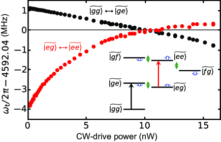
We first eliminate the residual ZZ interaction by the CW drive (Fig. 2). The drive frequency is 930 MHz, and the detuning from the transition is 84 MHz. The inset of Fig. 2 shows the shifts of eigenstates induced by the CW drive. The CW drive is red detuned from the transition and blue detuned from the and transitions. Thus, the sign of the frequency shift is different from each other. The amplitude of the ZZ interaction corresponds to the frequency difference between the and transitions, which amounts to MHz in the absence of the CW drive. The frequency difference vanishes at a certain power of the drive. It is also found that the CW drive does not degrade the coherence of the qubits (data not shown).
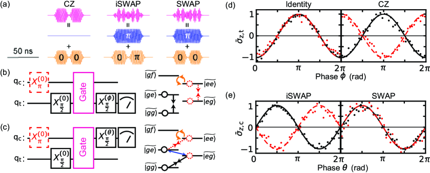
In the presence of the CW drive, we implement the two-qubit Clifford gate set, i.e. CZ, iSWAP and SWAP gates, using parametric couplings induced by additional microwave pulses. These gates are within the family of the Fermionic Simulation gate set, characterized by two parameters, the swap angle and the conditional phase fermi2018 ; martinis2020 . The CZ, iSWAP, and SWAP gates have the parameters , and , respectively. In our setup, and are independently and simultaneously controlled via parametric couplings.
Figure 3(a) illustrates the waveforms of the synthesized two-tone pulses for these gates. The total gate time is 50 ns for each. The swap pulse (blue) is resonant to the transition and is used to control . The control-phase pulse (orange) is resonant to the transition and controls through the relative phase between two serial segments, applying the conditional phase as a geometrical phase only to the state. Because the swap pulses also generate a small conditional phase due to the Stark shift, we simultaneously apply a control-phase pulse for iSWAP and SWAP gate to eliminate the unwanted phase.
Figure 3(b) [3(c)] shows the pulse sequence of the Ramsey interferometry for characterizing the identity and CZ gates [iSWAP and SWAP gates]. For the iSWAP and SWAP gates, which exchange an excitation between the qubits, we apply the second /2-pulse to the cubic transmon instead of the transmon to form an interferometric sequence [Fig. 3(c)], in contrast to the standard Ramsey experiments. Figures 3(d) and 3(e) show the experimental data of Ramsey oscillations, conditioned on the state of the cubic transmon, revealing the amount of the conditional phase of each two-qubit gate. The phase difference between the Ramsey oscillations, with and without an initial -rotation of the cubic transmon, corresponds to the conditional phase shift. The experimental data have good agreements with the ideal behaviors in Figs. 3(d) and 3(e).
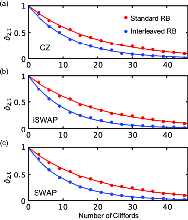
Finally, we characterize the average two-qubit gate fidelities with the randomized-benchmarking (RB) protocols RBth1 ; RBth2 ; RB1 . The gate time is uniformly set to 50 ns for the CZ, iSWAP, SWAP gates and all the single-qubit gates. Figure 4 shows the experimental results of the two-qubit RB. From the standard RB, the average gate fidelity of the two-qubit Clifford gates is determined to be . Using this value and those from the interleaved RB, we estimate the average gate fidelity of each two-qubit gate: , and for CZ, iSWAP and SWAP gates, respectively. The achieved fidelities of the two-qubit gates are comparable to those of the single-qubit gates supple and mostly limited by the energy relaxation time of the qubits. The coherence limits are approximately 0.97 according to the gate pulse widths, which are close to the observed fidelities. As the cubic transmon has basically the same layout as conventional transmons, we expect improvement of the relaxation time through optimizations of the design and fabrication.
In conclusion, we have demonstrated a parity-violated qubit called a cubic transmon, and realized microwave-controlled fast two-qubit gates between a cubic transmon and a conventional transmon. As the gates originate from the second-order nonlinearity of the circuit, the coupling strength scales inversely proportional to the detuning between the qubits, not to the square of it, and is thus sufficiently large for a wide detuning range of the qubits. This is advantageous for a multi-qubit system, which often suffers from a frequency-crowding problem. The residual static ZZ interaction is eliminated by applying a continuous microwave field, which will allow us to increase the bare coupling strength further and make the two-qubit gates as fast as 20 ns with optimal device parameters. This scheme for the suppression of the residual coupling can also be extended to multi-qubit systems as well as to higher-order interactions by using multiple drives.
The authors acknowledge Y. Sunada, K. Nittoh and K. Kusuyama for the help in sample fabrication and W. Oliver for providing a TWPA. This work was partly supported by JSPS KAKENHI (Grant Number 26220601, 18K03486), JST PRESTO (Grant Number JPMJPR1429), JST ERATO (Grant Number JPMJER1601), and Q-LEAP (Grant Number JPMXS0118068682).
References
- (1) R. Barends et al., Nature 508, 500 (2014).
- (2) F. Arute et al., Nature 574, 505 (2019).
- (3) S. S. Hong et al., Phys. Rev. A 101, 012302 (2020).
- (4) S. A. Caldwell et al., Phys. Rev. Appl. 10, 034050 (2018).
- (5) S. Sheldon, E. Magesan, J. M. Chow, and J. M. Gambetta, Phys. Rev. A 93, 060302(R) (2016).
- (6) M. D. Reed et al., Nature 482, 382 (2012).
- (7) J. Kelly et al., Nature 519, 66 (2015).
- (8) N. Ofek et al., Nature 536, 441 (2016).
- (9) L. Hu et al., Nat. Phys. 15, 503 (2019).
- (10) C. K. Andersen et al., npj Quantum Inf. 5, 69 (2019).
- (11) A. G. Fowler, M. Mariantoni, J. M. Martinis, and A. N. Cleland, Phys. Rev. A 86, 032324 (2012).
- (12) B. M. Terhal et al., arXiv:2002.11008 (2002).
- (13) A. O. Niskanen et al., Science 316, 723 (2007).
- (14) J. M. Chow et al., Phys. Rev. Lett. 107, 080502 (2011).
- (15) P. Krantz et al., Appl. Phys. Rev. 6, 021318 (2019).
- (16) S. Richer, N. Maleeva, S. T. Skacel, I. M. Pop, D. DiVincenzo, Phys. Rev. B 96, 174520 (2017).
- (17) M. Kounalakis, C. Dickel, A. Bruno, N. K. Langford, and G. A. Steele, npj Quantum Information 4, 38 (2018).
- (18) P. Mundada, G. Zhang, T. Hazard, and A. Houck, Phys. Rev. Appl. 12, 054023 (2019).
- (19) X. Han, T. Cai, X. Li, Y. Wu, Y. Ma, J. Wang, H. Zhang, Y. Song, and L. Duan, arXiv:2003.08542 (2020).
- (20) J. Ku et al., arXiv:2003.02775 (2020).
- (21) N. E. Frattini, U. Vool, S. Shankar, A. Narla, K. M. Sliwa and M. H. Devoret, Appl. Phys. Lett. 110, 222603 (2017).
- (22) N. E. Frattini, V. V. Sivak, A. Lingenfelter, S. Shankar, and M. H. Devoret, Phys. Rev. Applied 10, 054020 (2018).
- (23) V. V. Sivak, N. E. Frattini, V. R. Joshi, A. Lingenfelter, S. Shankar, and M. H. Devoret, Phys. Rev. Applied 11, 054060 (2019).
- (24) A. Noguchi, R. Yamazaki, Y. Tabuchi, and Y. Nakamura, Nat. Commun. 11, 1183 (2020).
- (25) P.-M. Billangeon, J. S. Tsai, and Y. Nakamura, Phys. Rev. B 91, 094517 (2015).
- (26) S. Richer and D. DiVincenzo, Phys. Rev. B 93, 134501 (2016).
- (27) F. Beaudoin, M. P. daSilva, Z. Dutton, A. Blais, et al., Phys. Rev. A 86, 022305 (2012).
- (28) J. Koch, T. M. Yu, J. Gambetta, A. A. Houck, D. I. Schuster, J. Majer, A. Blais, M. H. Devoret, S. M. Girvin, and R. J. Schoelkopf, Phys. Rev A, 76, 042319 (2007).
- (29) M. Aspelmeyer, T. J. Kippenberg and F. Marquardt, Rev. Mod. Phys. 86, 1391 (2014).
- (30) H. Häffner, C. F. Roos, and R. Blatt, Physics Reports 469, 155 (2008).
- (31) F. Mintert and C. Wunderlich, Phys. Rev. Lett. 87, 257904 (2001).
- (32) Supplementary Material
- (33) M. Ware et al., arXiv:1905.11480 (2019).
- (34) I. D. Kivlichan, J. McClean, N. Wiebe, C. Gidney, A. Aspuru-Guzik, Garnet Kin-Lic Chan, and R. Babbush, Phys. Rev. Lett. 120, 110501 (2018).
- (35) B. Foxen et al., arXiv:2001.08343 (2020).
- (36) E. Magesan, J. M. Gambetta, J. Emerson, Phys. Rev. Lett. 106, 180504 (2011).
- (37) E. Magesan et al., Phys. Rev. Lett. 109, 080505 (2012).
- (38) A. D. Córcoles, J. M. Gambetta, J. M. Chow, J. A. Smolin, M. Ware, J. Strand, B. L. T. Plourde, M. Steffen, Phys. Rev. A 87, 030301(R) (2013).
- (39) A. D. Córcoles et al., Nat. Commun. 6, 6979 (2015).
Supplementary Material for
“Fast parametric two-qubit gates with suppressed residual interaction
using a parity-violated superconducting qubit”
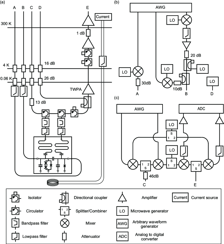
I Measurement setup
Figure S1 illustrates the wiring scheme for the gate experiments. The sample chip is connected to one readout port (C) and two drive ports (A, B). We apply microwave pulses generated by modulating the local oscillator signals. The qubits are simultaneously read out with the dispersive technique. The resonance frequencies and total decay rates of the readout resonators are 6.767 GHz and 0.8 MHz for the cubic transmon and 6.509 GHz and 1.0 MHz for the transmon, respectively. The reflection signals of the readout resonators are amplified by a Josephson traveling wave parametric amplifier (TWPA) and two low-noise amplifiers and demodulated for the readout. We apply a magnetic flux into the SNAIL loop through an external superconducting coil.
II SINGLE-PHASE APPROXIMATION OF CUBIC TRANSMON
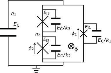
Figure S2 shows the full-circuit model of a cubic transmon. Each of the two isolated superconducting islands has two degrees of freedom of the phase and charge. The full Hamiltonian is written as
| (S1) | |||||
| (S4) | |||||
| C | (S7) |
where and are the numbers of excess Cooper pairs on each island, and are the superconducting phases across each junction connected to the ground, is the reduced magnetic flux, is the flux threading the loop, is the flux quantum, and () are the scaling factors depending on the junction size. is the single-electron charging energy of the shunt capacitance. We assume that each Josephson energy scales as , where is an independent parameter to be determined.
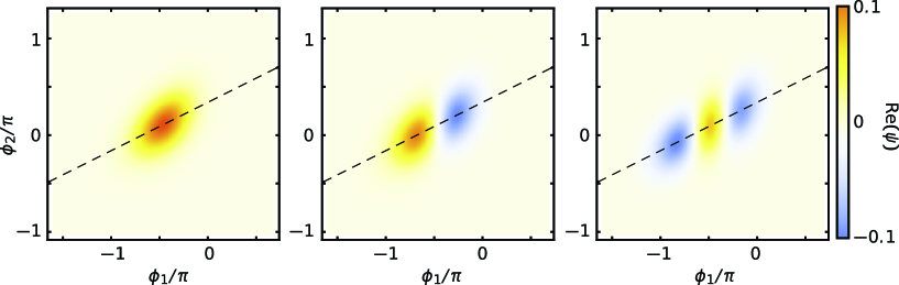
By diagonalizing the Hamiltonian, we obtain wave functions of the eigenstates of the cubic transmon in the phase representation (Fig. S3). Under the condition of , the fringes of the excited states lie on the dashed lines indicating the relation . The confinement of the wave functions along the dashed line suggests an approximation, , which we call the single-phase approximation. Using this relation, we can write the inductive energy of the SNAIL,
| (S8) | |||||
This gives an effective model with a single phase degree of freedom, . The Josephson energies in the main text are defined as and . The second formula in Eq. (S8) is the Taylor expansion around the phase at a minimum of the inductive energy, where is the relative phase variable for the expansion and are the expansion coefficients. The parity symmetry is broken as seen in the existence of the term in the presence of a finite magnetic flux penetrating through the SNAIL loop.
Under the approximation, the Hamiltonian of the cubic transmon up to the third-order nonlinearity is, as in the main text,
| (S9) |
where
| (S10) | |||||
| (S11) | |||||
| (S12) |
The effective charging energy is expressed as
| (S13) |
| Single-phase approximation | 0.21 | 84 | 0.070 | 0.20 |
| Full-circuit model | 0.18 | 103 | 0.070 | 0.20 |
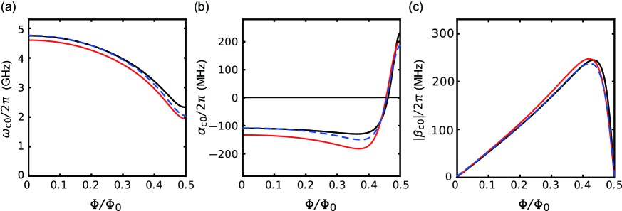
We quantitatively compare the single-phase approximation with the full-circuit model. We calculate the eigenmode frequency of the first excited state, , third-order nonlinearity and second-order nonlinearity of the cubic transmon based on each model (Fig. S4). For the calculation with the single-phase approximation, we use the parameters obtained by the fittings in Figs. S5(a) and (b) below. Next, we use the same parameters in the full-circuit model and compare the results (red lines). For the full-circuit model, the second-order nonlinearity is evaluated from the transition moment between the ground and second-excited states. The transition moment is defined as
| (S14) |
where . We also obtain from the perturbative approach
| (S15) | |||||
| (S16) |
where is the external drive amplitude for these transition. Using these, we calculate the absolute value of as
| (S17) |
The calculations based on these models qualitatively agree with each other [Fig. S4(a)–(c)] and demonstrate the validity and accuracy of the single-phase approximation. There is a small quantitative deviation between the two models, which is not surprising as the wave functions of the eigenstates (Fig. S3) are not completely localized along the dashed line. This means that is not strictly satisfied because of the quantum fluctuation of , and we cannot construct an exact single-phase model. Blue dashed curves in Fig. S4 show calculations based on the full-circuit model with adjusted parameters to reproduce the results of the single-phase approximation. For the region with small reduced magnetic flux, these calculations have a good agreement with each other.
III COUPLED QUBITS
As described in the main text, the total Hamiltonian of the cubit-transmon–transmon coupled system is given as
| (S18) | |||||
| (S19) | |||||
| (S20) |
The parameters are defined in the main text. We treat the off-diagonal part as a perturbative term and obtain the effective Hamiltonian via Schrieffer-Wolff transformation.
| (S21) |
We introduce which fulfills
| (S22) |
Then, the effective Hamiltonian in the second order reads
| (S23) |
We calculate the effective Hamiltonian by ignoring states with more than four excitation quanta in each qubit and truncating it into a matrix with elements for the two-qubit system. The calculation is valid when and are satisfied. The effective Hamiltonian reads [Eq. (2) in the main text]
| (S24) |
where , , , and are the eigenmode frequencies and self-Kerr nonlinearities of the qubits after the perturbative treatment of the coupling term. They are expressed as follows:
| (S25) | |||||
| (S26) | |||||
| (S27) | |||||
| (S28) |
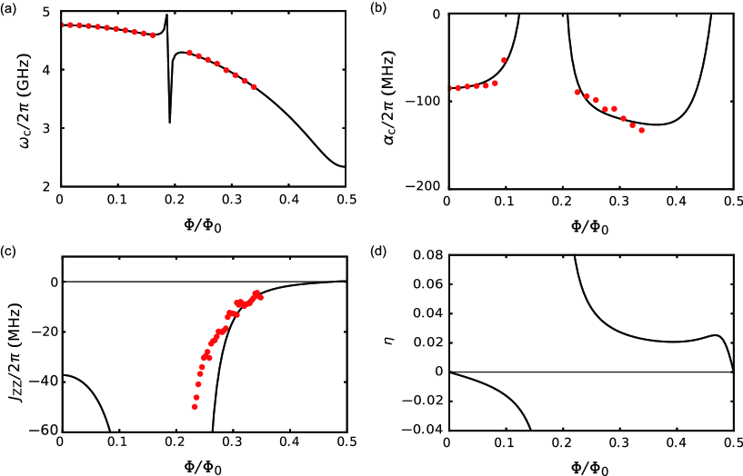
where is the detuning between the qubit bare frequencies. We use these expressions to fit the experimental data, as shown in Figs. S5(a) and S5(b). The fitting parameters are listed in Table S1.
The term in the effective Hamiltonian [Eq. (S24)] is the parity-violating term, and the effective couping strength is expressed as
| (S29) |
The amplitude of the residual ZZ interaction, , between the qubits is derived through Schrieffer-Wolff transformation up to the fourth order of ,
| (S30) | |||||
| (S31) |
In Fig. S5(c), we plot obtained with the parameters that are determined from the fittings in Figs. S5(a) and S5(b). In the dispersive regime of the two qubits, i.e., for , the experimental data in Fig. S5(c) has a good agreement with the theoretically expected values.
For the calculation of the parametric coupling, we continue this procedure one more step. We set such that
| (S32) |
where is the off-diagonal part of the effective Hamiltonian . We drive this system at the frequency with a phase , such that
| (S33) |
and transform the drive Hamiltonian as
| (S34) |
to obtain the parametric coupling of the SWAP interaction for [Eqs. (3) and (4) in the main text],
| (S35) | |||||
| (S36) |
For the CZ gate, we use the transition at involving the second-excited state of the transmon, whose amplitude is similarly obtained as
| (S37) |
IV PARAMETRICALLY-INDUCED transition
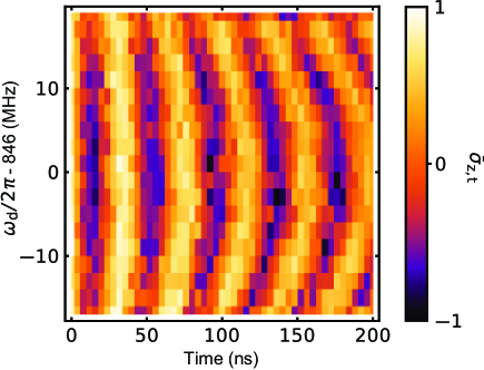
Figure S6 shows the experimental data of the parametrically-induced transition. We prepare the state with a -pulse to the cubic transmon and apply the parametric drive to the cubic transmon. The excitation is swapped between the two states by the parametric transition. The resonance frequency, 846 MHz, is the frequency difference between eigenfrequencies of the cubic transmon and transmon. The Rabi frequency is proportional to the amplitude of the drive, and the maximum Rabi frequency of 30 MHz is obtained.
V Randomized Benchmarking
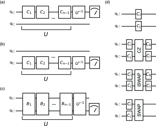
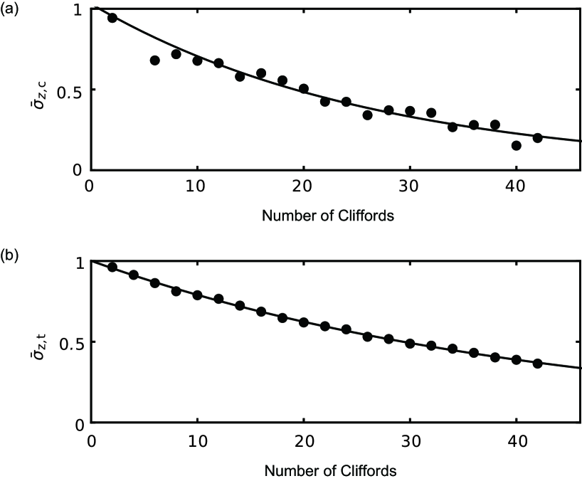
Figure S7 shows the gate sequences for the single-qubit and two-qubit randomized benchmarking (RB). We drive the cubic transmon with a CW field to eliminate the static ZZ interaction (not shown). The pulse shapes for the single-qubit gates are Gaussian with a full width at half maximum of 18.6 ns. The swap pulse and each segment of the control-phase pulse [Fig. 3(a) in the main text] have rising and falling edges of a Gaussian shape with the half width at half maximum of 3.0 ns and 1.5 ns, respectively. The length of the flat-top region is 32 ns for the swap pulse and 16 ns for each segment of the control-phase pulse.
The tails for all pulse are truncated when the amplitudes become times smaller than the maximum. For the interleaved RB, we add a target gate (CZ, iSWAP and SWAP) between each Clifford gates. We repeat the sequences 5000 times with 100 (50) different random patterns for the protocol in Figs. S7(a) and S7(b) [Fig. S7(c)]. We measure the average value of the -component of the cubic transmon in the protocol in Fig. S7(a) and that of the transmon in Figs. S7(b) and S7(c).
Figure S8 shows the results of standard RB for the single-qubit gates. The average gate fidelities of the single-qubit gates are evaluated to be for the cubic transmon and for the transmon.
VI Raman transition through a CONTINUOUS MICROWAVE field
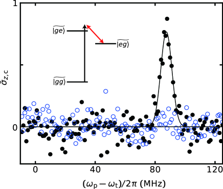
In the main text, we irradiate the cubic transmon with a continuous microwave (CW) drive to eliminate the unwanted static ZZ interaction between the two qubits. However, this CW drive also induces an unwanted Raman transition which is mediated by the transmon excitation. Figure S9 shows the experimental data regarding the transition with pulsed spectroscopy. We sweep the frequency of the probe microwave pulse, , around the transmon excitation frequency and measure the state of the cubic transmon. The pulse has a Gaussian shape with the full width at half maximum of 60 ns. The peak observed in Fig. S9 corresponds to the Raman transition process depicted in the inset. In accordance with the CW-drive detuning of 84 MHz from the transition, the Raman transition appears at MHz. This transition is close to the transmon resonance and can be an error source for single-qubit gates with a short pulse. This error can be suppressed by the use of DRAG pulses DRAG .
References
- (1) F. Motzoi, J. M. Gambetta, P. Rebentrost, and F. K. Wilhelm, Phys. Rev. Lett. 103, 110501 (2009).