Fast prediction and evaluation of eccentric inspirals using reduced-order models

The CBwaves open-source software was developed by the Virgo Group at Wigner Research Centre for Physics with the intent of providing efficient computational tool capable of generating gravitational waveforms produced by generic spinning binary configurations moving on eccentric closed or open orbit within the applied PN framework. A detailed examination of the software’s performance is given in Ref. Csizmadia et al. (2012). The source release and binary packages supported both on x86 and x86_64 platforms are available at the group’s website Csizmadia et al. (2011).

In the PN formalism the spacetime is assumed to be split into the near and wave zones. The field equations for the perturbed Minkowski metric are solved in both regions. A fourth-order Runge–Kutta (RK4) method with adaptive step-size control is carred out to numerically solve for the 3PN-accurate near-field radiative dynamics at each time $t>t_{0}$, where $t_{0}$ is the time of arrival of the signal at the detector, while the far-zone radiation field Kidder (1995) decomposed as

is determined in harmonic coordinates by a simultaneous evaluation of orbital elements $(\phi,\,r,\,n)$ where $D$ is the distance (typically a few Mpc) to the GW source of that consists of two point particles of masses $m_{1}$ and $m_{2}$ and $\mu=m_{1}m_{2}/M$ is its reduced mass. The term $Q_{ij}$ is the Newtonian mass quadrupole moment, $P^{0.5}Q_{ij},\,P^{1.5}Q_{ij},\,P^{2}Q_{ij}$ are higher-order relativistic corrections up to 2PN order beyond the Newtonian term while $PQ_{ij}^{\text{SO}},\,P^{1.5}Q_{ij}^{\text{SO}},\,P^{2}Q_{ij}^{\text{SS}}$ are corrections arising from spin–orbit and spin–spin effects, respectively. Here, for brevity, we will not repeat lengthy PN coefficients. They are written out explicitly in the appendix of Ref. Csizmadia et al. (2012).

Radiative orbital dynamics involving all possible correction terms up the 3PN order beyond the Newtonian term are written out explicitly in terms of mean motion $n$ and orbital eccentricity $e$ in Ref. Königsdörffer and Gopakumar (2006). The secular evolution is treated adiabatically, assuming that the timescales of the shrinkage of orbits (due to gravitational energy radiation $\dot{E}$) and the precession (due to angular momentum flux $\dot{J}$) are much longer than that of the orbital period. Consequently, the functions $(\dot{x}_{\text{1PN}},\,\dot{e}_{\text{1PN}}\ldots)$ in the equations derived from $\dot{E}$ and $\dot{J}$ depend only on the eccentricity $e$, and not on eccentric anomaly $u$. Hence, the adiabatic evolution equations for $x\equiv(M\omega)^{2/3}$ and $e$ form a closed system, and can be solved independently of the Kepler’s equation. Given initial conditions $x(0)$ and $e(0)$, we can solve the system of ordinary differential equations numerically to obtain $x(t)$ and $e(t)$. The integration of the equations of motion is terminated at the innermost stable circular orbit (ISCO), which is located at

in Schwarzschild spacetime (for a non-spinning NS/BH). The orbital angular frequency at the ISCO is

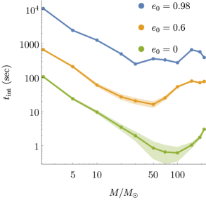
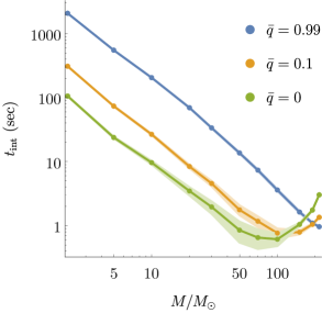
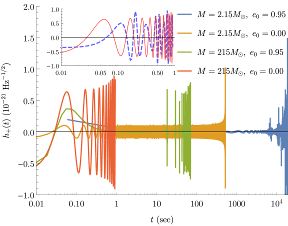
which marks the end of the inspiral phase. Fig. 1 demonstrates that the integration run-time $t_{\text{int}}$ depends sensitively both on the initial eccentricity and on the disparity of components’ masses $(m_{1},\,m_{2})$ in a binary system. The $t_{\text{int}}$ increases exponentially with decreasing total mass $M$. The mass disparity, defined by $\bar{q}\equiv 1-q$, allows better comparability with $e_{0}$ than $q$ itself, considering that $t_{\text{int}}$ asymptotically increases – faster than with decreasing $M$ – towards infinity as either $e_{0}$ (left panel) or $\bar{q}$ (right panel) tends to 1. The physical interpretation of these competing trends is very simple:

1. 1.

   The lighter the components of the binary are, the longer it takes for them to gradually descend onto their ISCO through a sequence of increasingly circular orbits. Pfeiffer (2012)

2. 2.

   The more eccentric the orbit was initially, the longer it takes to shed its residual eccentricity over many orbital periods. Peters (1964)

3. 3.

   Among different configurations of equal total mass, the one with the largest mass disparity has the longest inspiral time for harbouring the lightest component. Pfeiffer (2012)

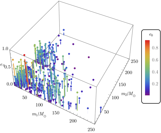
At the high total-mass region on Fig. 1, the influence of first trend grows comparable to that of the last two to reverse the trend of decreasing integration run-time. Fig. 3 shows the influence of $M$ and $q$ on the length of integration run-time $t_{\text{int}}$ from a different aspect. Excluding the red and yellow dots, each point in the coloured triangular region is assigned to a hue level running from dark to light as the value of $t_{\text{int}}$ increases on a logarithmic scale. The dark blue ‘basin’ represents the region where $M$ and $q$ simultaneously lower the value of $t_{\text{int}}$ to its minimum. Isoclines running in parallel are connecting points at which $t_{\text{int}}$ has the same value, therefore they are associated with horizontal lines in Fig. 1 (b). The influence of growing $q$ becoming comparable to and gradually greater than that of $M$ accounts also for the drift from the linear rising trend in the curvature of isoclines that occurs at the high-$q$ region on Fig. 3. Although Fig. 3 suggests that over $85\%$ of the waveform templates of initial eccentricity $e_{0}=0$ are computed up to $10$ seconds, in fact, only $4.6\%$ of all waveform templates require less then $10$ seconds to integrate, as demonstrated in Fig. 2. Out of a total of 1800, only those 120 templates are shown in Fig. 3 that are located in the $e_{0}=0$ plane. Still, the figure illustrates well that in the same $e_{0}$-plane the frequency of templates with little $t_{\text{int}}$ is extremely high compared to that of templates with large $t_{\text{int}}$, regardless of the value $e_{0}$.

In the next section we shall give a quantitative description of the summary statistics computed from the relative frequency of occurrence (or empirical probability) of the integration time-runs.

Let $\mathbb{T}=\{t^{\text{int}}_{1},\,t^{\text{int}}_{2},\ldots,\,t^{\text{int}}_{L}\}$ be a univariate independent and identically distributed (IID) finite data sample drawn from the probability (or relative frequency) distribution of the discrete random variable $t\in\mathbb{T}$ while a discrete set of $L$ time-domain input waveforms

is computed at each parameter point $\lambda_{l}$ (see Sec. III.1) by evaluating eq. (1) at a distance $D=\mu$ simultaneously with the integration of the equations of motions at 3PN order that requires integration run-times $t^{\text{int}}_{l}$.

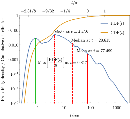
Since we do not make any prior assumption about the probability distribution, we shall use a non-parametric model where the statistical measures are determined by the finite data sample $\mathbb{T}$. In statistics, kernel density estimation (KDE) is a fundamental data-smoothing technique that provides a non-parametric estimate, based on observed data $\mathbb{T}$, of an unobservable underlying probability density function (PDF) of the continuous random variable $\inf\mathbb{T}\leq t\leq\sup\mathbb{T}$. A PDF, denoted by $\mathscr{f}_{t}$ and illustrated in Fig. 2, is a non-negative Lebesgue-integrable function that defines the cumulative distribution function (CDF) of a real-valued random variable $t$, evaluated at a value $t^{\prime}$ as

It represents the probability that the random variable $t$, with the expected value given by

takes on a value less than or equal to $t^{\prime}$ and its kernel density estimator is

where $K\geq 0$ is a symmetric kernel with total integral normalized to unity and $h>0$ is the bandwidth (or smoothing parameter). One might intuitively choose $h$ as small as the data sample $\mathbb{T}$ allows; however, there is always a trade-off between the bias of the estimator and its variance. Another option is the use of adaptive bandwidth kernel estimators in which the bandwidth changes as a function of $t$.

A specific quantitative measure of the probability distribution is the $n$-th moment

of the continuous random variable $t$ about some central value $c$ (e.g. the mean, denoted by $\mu$) where $E$ is the expected value of $t$ defined by eq. (6). The graphical representation of the most common measures of central tendency (mean, median, mode) is depicted on Fig. 2 with solid, dashed and dotted red lines, respectively. The PDF rapidly increases with the random variable $t$ up to a point at $t=0.81653$ sec. From then onwards this monotone increase slows down and eventually comes to a halt at $t=4.438$ sec, which marks the mode, i.e. the most frequent value in the distribution. The median which represents the value separating the higher half of the probability distribution from the lower half is located at $t=20.615$ sec. The mean which represents the first moment of the PDF ($\mu\equiv\mu_{1}$ in eq. (8)) is situated at $t=77.499$ sec.

The central tendency of distributions is typically contrasted with its dispersion that measures the extent to which a distribution stretched or squeezed. Common measures of statistical dispersion are the variance and standard deviation: The variance of $t$ is the second central moment, given by (8) as $\operatorname{Var}[t]\equiv E[(t-\mu)^{2}]$ and the standard deviation is its square root, denoted by $\sigma$. For the given distribution $\sigma=266.885$ sec. Finally, the shape (or asymmetry) of probability distributions is quantitatively measured by the third and fourth central moments, called skewness and kurtosis and denoted by $\operatorname{Skew}[t]\equiv E[(t-\mu)^{3}/\sigma^{3}]=18.56$ and $\operatorname{Kurt}[t]\equiv E[(t-\mu)^{4}/\sigma^{4}]=490.04$, respectively.

The set of input waveforms (4) is computed by CBwaves, described in Sec. II.1, at corresponding parameter points

in a compact $p$-dimensional parameter space $\Omega\subset\mathbb{R}^{p}$ where $p$ is the number of model parameters. We restrict ourselves to a feasible 3-dimensional parameter space consisting of totally ordered one-dimenstional sets of values of corresponding model parameters $(m_{1},\,m_{2},\,e)$ that define a sparse grid of points

covering the desired parameter range in the particular model involved. Owing to the invariance of input waveforms under exchange of the components’ masses $(m_{1},\,m_{2})$, the values of the 2-dimensional index pair $(i,\,j)$ are constrained to a triangular sub-region in the positive quadrants where $i\leq j$. Considering that the waveform templates span a 3-dimensional parameter space, each template is successively placed into a single vector (4) as indexed by

in the range of values $1\leq l\leq L$. This flat index corresponds to the position of templates in the parameter space. The total number of templates in the set is then expressed as

It is desirable to work with a dense grid of short waveforms encompassing the late inspiral phase to make a better coverage of the selected region of the parameter space. For the sake of simplicity, we sample at equidistant parameter combinations within the region. Nevertheless, using a template placement algorithm that is based on a template-space metric over the parameter space makes a far more efficient coverage. Kalaghatgi et al. (2015); Cokelaer (2007) Generally, the algorithms that use geometrical techniques concentrate more points near the boundaries of the region and at lower mass-ratios.

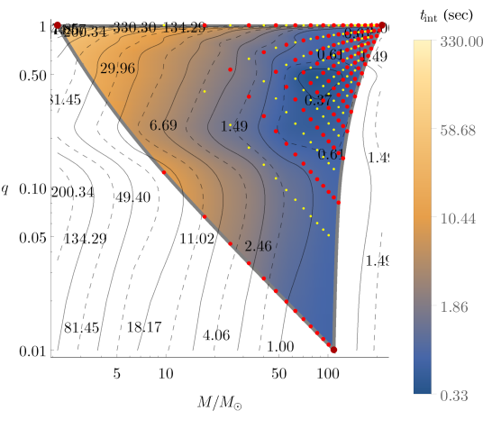
The set of initial eccentricity $\{e_{k}:1\leq k\leq k_{\text{max}}\}$ is chosen to cover the entire interval $[0,\,0.95]$ and the mass ratio $q\equiv m_{1}/m_{2}\leq 1$ is allowed to range between equal mass at $q=1$ and relatively extreme systems at $q\approx 0.01$ with total mass $M/M_{\odot}\in[2.15,215]$. In terms of the symmetric mass ratio $\eta=\mu/M$ the model covers approximately $\eta\in[0.01,0.25]$. Fig. 3 shows the placement of those $L=120$ templates (red dots) that are situated in the $k=0$ plane section of the parameter space $\Omega$, out of a total of $1800$ templates and are collected in $\bm{h}(t)$. These templates are confined within a triangular region with a boundary $\partial\Omega$ (thick gray line).

For optimal orientation all time-domain waveforms in eq. (4), composed of their two fundamental polarizations $h_{+}$ and $h_{\times}$ in the dominant $\mathscr{l}=\mathscr{m}=2$ mode are represented by complex-valued GW strain amplitudes

at $N$ equidistant grid points

as elements of a finite sequence of $N$ regularly spaced samples of the complex-valued TD waveforms $\{h_{0}(\lambda_{l}),\,h_{1}(\lambda_{l}),\,\ldots,\,h_{N-1}(\lambda_{l})\}$. The sequence is converted by a fast Fourier transform (FFT), denoted by a linear operator $\mathscr{F}:h\to\tilde{h}$, into an other equivalent-length sequence of regularly spaced samples

evaluated at the same $N$ equidistant frequency grid points $\{f_{-N/2},\,\ldots,\,f_{0},\,\ldots,\,f_{N/2-1}\}$ considering that ROM construction, to be discussed in Sec. IV, will require a set of values that reside in the same grid points over all the waveforms in the template bank.

1. 1.

   This is achieved by having the length of all frequency series truncated to that of the shortest waveform in time, denoted by

   $$T=t_{N-1}-t_{0}.$$

   (16)

   This particular waveform is associated with the highest mass, lowest eccentricity configuration $(i=i_{\text{max}},\,j=i_{\text{max}},\,k=0)$ in the template bank and its position in the parameter space, given by eq. (11), is $l_{\text{short}}=(i_{\text{max}}+3)i_{\text{max}}k_{\text{max}}/2+1$.

2. 2.

   Another possible way, used by Pürrer (2014, 2016), to adjust the frequency series to the same length is to make the shorter-length waveforms of sufficient length by extending them with other templates such as TaylorF2.

The Fourier coefficients in eq. (15), given by

are complex-valued functions of the frequency $f_{k}$ which encodes both the amplitude and the phase,

respectively. In this interpretation, $\tilde{h}_{k}(\lambda_{l})$ corresponds to the cross-correlation of the time sequence $h_{n}(\lambda_{l})$ and an $N$-periodic complex sinusoid $e^{2\pi ikn/N}$ at a frequency point $f_{k}\equiv k/N$ that represents $k$ cycles of the sinusoid. Therefore, eq. (17) acts in place of a matched filter for that frequency. Now, the sequence of frequency-domain waveforms (15) can be re-expressed as ‘chirps’ in a simple form

where the oscillation degree $\Lambda$ is a large number. The behavior of GWs in the late inspiral phase is highly oscillatory, but the amplitude and the phase themselves are smoothly varying functions of frequency. Candes et al. (2008) It will thus be more expedient to perform high-accuracy parametric fits of the phase and amplitude given by (18) rather than of the complex waveform (13) itself. The preprocessed amplitudes and phases are collected in the columns of separate template matrices $\{\mathcal{H}^{(A)},\,\mathcal{H}^{(\phi)}\}\in\mathbb{R}^{N\times L}$,

where we have droped the amplitude or phase labels for brevity and where $L$ is the total number of templates, and each template $\tilde{h}_{l}(f_{k})$ is given on a common freqency grid of length $N$. We may choose to represent the waveforms at a large number of frequency points so that $N\gtrsim L$.

Provided that $T$ in (16) is the longest time length, the time spacing is defined as

by eqs. (14) and (16). The time spacing and the number of time steps $N$ in the grid (14) are chosen such that the FD waveforms (19) are sampled at a rate of $f_{\text{s}}$ and cover a suitable and well-resolved frequency range $[f_{\text{low}},f_{\text{high}}]$.

1. 1.

   The lower limit of the frequency range $f_{\text{low}}$ is specified by the low-frequency cutoff of the detector noise spectrum which is close $f_{\text{cutoff}}=10$ Hz for advanced detectors design.

2. 2.

   The upper limit $f_{\text{high}}$ is determined to be at $f_{\text{ISCO}}=2.045$ kHz by the ISCO frequency (3) for the lowest total mass configuration of interest $M=2.15M_{\odot}$.

The Nyquist criterion requires the sampling frequency to be at least twice the highest frequency contained in the signal to avoid aliasing. Thus, the smallest sufficient sampling frequency is $f_{\text{s}}=4096$ samples per second for being the first power of 2 to meet the criterion. Note that the typical sampling rate being used by aLIGO and aVirgo observatories in ongoing searches for GWs is at 2048 Hz. Aasi et al. (2013) Instead, an equidistant grid with $N=4000$ grid points is sampled at $f_{\text{s}}=16.384$ kHz in the frequency band $Mf\in[0.0001,0.0216]$ in geometric units $(G=c=1)$. The total mass $M$ is expressed in units of geometrized solar mass by $M_{\odot}[\text{s}]=G/c^{3}\times M_{\odot}[\text{kg}]\approx 4.93\times 10^{-6}$ sec. At the time resolution $\Delta t=1/f_{\text{s}}\approx 4.59M$ which corresponds to a Nyquist frequency

a waveform long enough for the BNS system of total mass $M=2.15M_{\odot}$ down to $f_{\text{low}}=2.48\times 10^{-35}M^{-1}$ is given and is about $T=(N-1)\Delta t\approx 1.83\times 10^{4}M$ long in time. The spacing in frequency domain is

so the power will be either in positive or negative frequencies, depending on conventions and we need to consider only half of the FFT. Combining this with the relations (21–22), one has

Only half of the points in the FFT spectrum are unique, the rest are symmetrically redundant. Thus, the points of negative frequencies contain no new information on the periodicity of the random number sequence. Which amounts to swapping the left and right half of the result of the transform.

Formally, the decomposition of the template matrix $\mathcal{H}\in\mathbb{C}^{N\times L}$ in eq. (20) is expressed by a factorization of the form

where the complex unitary matrices

are orthogonal sets of non-zero eigenvectors of the non-negative self-adjoint operators $\mathcal{H}^{\dagger}\mathcal{H}$ and $\mathcal{H}\mathcal{H}^{\dagger}$ so that $U^{\dagger}U=\mathbb{I}$ and $V^{\dagger}V=\mathbb{I}$. The rank–nullity theorem states that the SVD (25) provides a decomposition of the range of $\mathcal{H}$. Pürrer (2014) Accordingly, the left-singular vectors (or eigensamples) $\{\bm{v}_{i}\in V\}$ provide an orthonormal basis

for the range of $\mathcal{H}$ (columnn space) where the maximal number of linearly independent columns of $\mathcal{H}$ is $R\equiv\operatorname{rank}(\mathcal{H})\leq L$. In a qualitative sense, each $\bm{v}_{i}$ represents a typical waveform pattern. The right-singular vectors (or eigenfeatures) $\{\bm{u}_{i}\in U\}$ provide a basis for the domain of $\mathcal{H}$ (row space) and represent the evolution of the magnitude of each waveform along the frequency gridpoints. The diagonal entries of the rectangular matrix $\Sigma\in\mathbb{R}^{N\times L}$ correspond to the non-negative real singular values (SVs) $\sigma_{1}\geq\ldots\geq\sigma_{s}\geq 0$ where $s=\min(N,L)$. SVs are roots of eigenvalues of $\mathcal{H}^{\dagger}\mathcal{H}$ (and of $\mathcal{H}\mathcal{H}^{\dagger}$) describing the spectrum of the template matrix $\mathcal{H}$, arranged in monotonically decreasing order (see Fig. 5). If the number of frequency points is significantly larger than the number of waveforms (i.e. $L\ll N$) then a thin SVD is a more compact and ‘economical’ factorization of eq. (25) than the full-rank SVD that comprizes all $R$ eigensamples. In practice, low-rank matrices are often contaminated by errors, and for that reason they feature an effective rank $R_{\text{eff}}$ smaller than its exact rank $R$. The reduced-rank approximation of the template matrix $\mathcal{H}$ is expressed by

which comprises only those $r<R$ singular vectors which correspond to singular values of a significant magnitude. The approximated representation (28) of the fiducial template bank $\mathcal{H}$ is the $r$-th partial sum of the outer-product expansion of the expression (25) where $r$ denotes the desired target rank. The Eckart–Young theorem Eckart and Young (1936) implies that the low-rank SVD in eq. (28) provides the optimal rank-$r$ reconstruction of the template matrix

in the least-square sense where the truncation error of approximated representation (28) in both the spectral and Frobenius norm is given by

respectively.

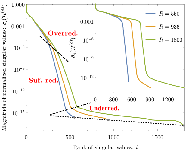
Fig. 5 shows $\hat{\sigma}_{i}\equiv\sigma_{i}/\sigma_{1}$ on logarithmic scale as a function of the number of SVD components $i=\{1,\ldots,R\}$ involved in the approximated representation. Each $\hat{\sigma}_{i}$, which describes the relative magnitudes of the corresponding eigenfeatures, is computed from the truncated SVD (28) of template matrices with three distinct full-ranks $R=\{550,\,936,\,1800\}$ (i.e. total number of templates). The truncation error in the approximation, in accordance with eq. (30), decreases with the number of SVD components retained. The ultimate accuracy (or minimal error) achievable is limited by the total number of templates $L$ that the original template matrix $\mathcal{H}$ contains. The growing rate of decay in the SV spectrum demonstrates that the individual SVD components gradually lose their relevance for being included in the approximation. In this respect, the spectrum has three clearly distinctive regions characterized by the rate at which SVs decrease:

1. 1.

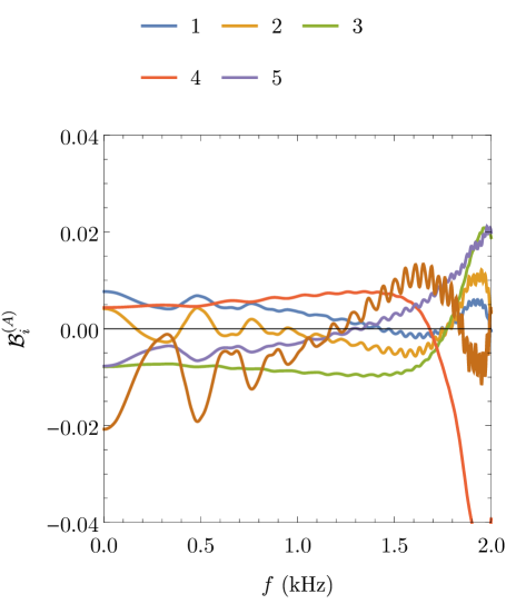
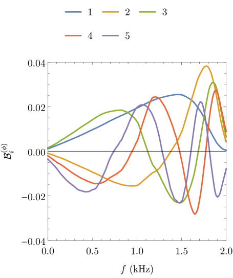
   Overreduced SVDs $(k\lesssim 400)$ retain insufficient amount of information to construct a representation by the orthonormalization (27) with less than relative error of $10^{-5}-10^{-6}$. The initial steep exponential fall attests that the information contained in the corresponding eigenfeatures is predominantly relevant. In fact, the first few components shown on Fig. 6 contain roughly $90\%$ of all the information on the input waveforms, regardless of $\operatorname{rank}(\mathcal{H})$. Then, SVs decrease at a much lower, yet a slowly increasing rate, practically indistinguishable for different values of full rank $R$.

2. 2.

   Sufficiently reduced SVDs $(400\lesssim k\lesssim 500-600)$ efficiently select the relevant information, so that the relative error of representation (41) is kept well-suppressed while the number of SVD components stored in the reduced-rank template matrix is significantly lower than that of the full-rank. The larger the full-rank $R$ is, the more SVD components have to be kept to achieve the same accuracy of representation.

3. 3.

   Underreduced SVDs $(k\gtrsim 500-600)$ admit the lowest possible truncation errors, limited only by the numerical errors of the full-rank approximation itelf. However, the accuracy of reconstructed waveform representation improves at a rate much lower than in the preceding regions. The loss of relevant information content due to the reduction of the number of SVD components is inefficiently low compared to the improvement of accuracy.

Choosing an optimal target rank $r$ is highly dependent on the objective. One either desires a highly accurate reconstruction of the fiducial waveform templates, or a very low dimensional representation of the fundamental features in the templates. In the former case $r$ should be chosen close to the effective rank, while in the latter case $r$ might be chosen to be much smaller. Fig. 5 demonstrates that choosing a target rank $r=456$ for the smallest among fiducial template matrices will result in a truncation error related to $\hat{\sigma}=2.66\times 10^{-15}$ at $r=456$.

The basis for the amplitude or phase space is given in the columns $\mathcal{B}_{i}$ of the matrix

and a full-rank basis is desired. If $N<L$, then the information from $L$ waveforms at $N$ grid points is contained in a basis of dimension $N$. The reduced basis waveforms only resemble the physical behavior of frequency domain amplitudes and phases for the first basis function, the higher basis functions are oscillatory (see Fig. 6). To compress the model, a reduced basis of rank $r$ is selected from the full-rank basis (27) in the form

For any $r$ the columns of $V_{r}$ are an optimal orthonormal bases for the starting waveforms. Notice that $\mathcal{B}_{r}\subset\mathcal{B}_{r+1}$, which demonstrates the underlying hierarchical nature of the generated template banks. Pürrer (2014) Fig. 7 may serve as an illustration of the underlying sparsity of the selected basis in the parameter space. The identification of parameter values associated with the basis waveforms selected by SVD from the full template bank is not that straightforward as a greedy algorithm would pick values that parameters take. Nevertheless, it may safely be said that a very small part of the parameter space volume is covered; the parameter points are heavily concentrated at low-mass and low-eccentricity values.

Hereafter the label $r$ on the rank-$r$ reduced basis will be dropped for brevity. Given the reduced bases $\mathcal{B}^{(A)}$ and $\mathcal{B}^{(\phi)}$, we compute projection coefficient vectors $\vec{\mu}$ for any given input waveform $\tilde{h}\in\mathbb{R}^{N}$ as follows

where the labels referring to amplitude or phase were dropped for brevity. The projection coefficient vectors for all waveform templates are packed in the matrices $\mathcal{M}^{(A)}$ and $\mathcal{M}^{(\phi)}$ with entries

Comparing with eq. (25) we see that $\mathcal{M}=\mathcal{B}^{T}\mathcal{H}=-\Sigma U^{T}$ for a full-rank basis $\mathcal{B}=V$. It follows that the projection coefficient matrices are ordered in the same way as the individual waveforms in $\mathcal{H}$. To undo the packing of the waveforms in the matrices $\mathcal{M}$ we just partition the linear index $l$ that enumerates the waveforms in $\mathcal{H}$ and obtain a tensor

To complete the model we define the projection coefficient vectors at any position in the chosen parameter space by suitable interpolants $I[\mathcal{M}](\lambda)\in\mathbb{R}^{r}$ for the amplitude and phase coefficient tensors $\mathcal{M}^{(A)},\,\mathcal{M}^{(\phi)}$. For each input waveform we have two corresponding $r$-vectors of projection coefficients (for amplitude and phase) that are interpolated over the parameter space. The frequency-domain ROM representation of waveform templates is then constructed in the form

where $\cdot$ denotes matrix multiplication, $I_{f}[\cdot]$ interpolates vectors in frequency on a suitable grid, and $A_{0}(\lambda)$ is an amplitude prefactor which is stored before the SVD takes place and an interpolant is computed over the parameter space.

The overlap integral of two normalized waveforms, say, of a fiducial CBwaves waveform $h_{\text{CB}}$ and its surrogate model prediction $h_{\text{S}}$, is given by the mismatch (or unfaithfulness) between the two waveforms and is defined as the normalized inner product (38) maximized over time and phase shifts

with an inherited norm given by $\lVert h\rVert^{2}\equiv\langle h,h\rangle$. A natural inner product between the two waveforms is given by the complex scalar product

where the tilde denotes Fourier transformation given in eq. (15), $\tilde{h}_{\text{S}}^{*}(f)$ is the complex conjugate of $\tilde{h}_{\text{S}}(f)$, $S_{\tilde{h}}(f)$ is the one-sided power spectral density (PSD) of the detector noise and $f_{\text{low}}$, $f_{\text{high}}$ are suitable cutoff frequencies for detector sensitivity. The low-frequency cutoff depends on the PSD and is at $10$ Hz for advanced detectors design. The high-frequency cutoff is at $2.045$ kHz, which is the ISCO frequency of the lowest total-mass configuration in our fiducial model, discussed in Sec. III.3.

A discrete version of the normed difference between a fiducial waveform and its surrogate is what we can actually measure:

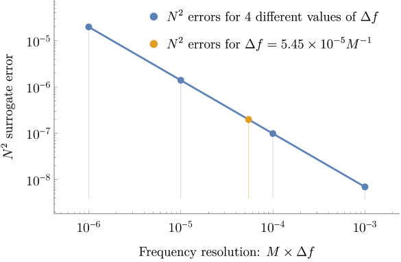
where $f_{s}$ is the sampling frequency discussed in Sec. III.3. The square of the normed difference between two waveforms, refered to as the surrogate error, is directly related to their overlap (38). It is the dominant source of error in the surrogate model that translates directly into errors in the fits of the parameters for building the surrogate. Field et al. (2014) Fig. 8 shows the linear correlation of the surrogate error in eq. (39) with the time spacing $\Delta f$ in the regularly spaced grids (14–15). The surrogate model gradually converges to the fiducial one at finer time scales (i.e. larger sampling frequencies). Other errors of interest are the pointwise ones (separately for the amplitude and phase). They are encoded in the $l$th surrogate model prediction (36) as

respectively. The relative errors in approximating the amplitude and phase of a fiducial waveform by its surrogate model prediction is then expressed by

where the amplitude and phase parts of fiducial waveforms, $\tilde{h}^{(A)}_{\text{CB}}(f_{k};\lambda_{l})$ and $\tilde{h}^{(\phi)}_{\text{CB}}(f_{k};\lambda_{l})$, respectively, are given by eq. (18) on $N$ discrete frequency points $f_{k}$.

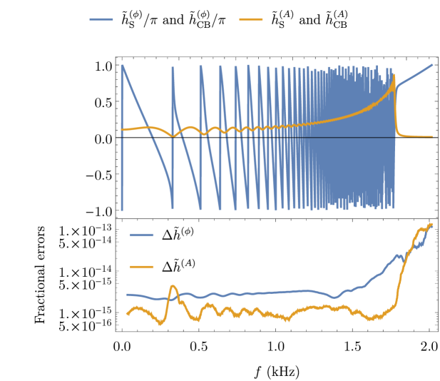
Fig. 9 shows a comparison between the surrogate and fiducial model, using the template assigned to $l=1$. The top panel shows that the fiducial and surrogate waveforms are visually indistinguishable. The bottom panel demonstrates that both amplitude and phase pointwise errors (41) increase with frequency. Nevertheless, the errors are indeed as small as predicted on Fig. 5. A moving average of $50$ points was used to smooth out short-term fluctuations in the error and highlight longer-term trends.

Apart from the requirements for accuracy or reliability, a ROM building is considered efficient if it generates cost-efficient surrogate models. The major advantage of using surrogate model predictions in lieu of actual waveform evaluations is their significantly reduced resource consumption. Now we discuss the computational cost, in terms of operation counts and run-time, of ROM building and present the desired speedup that can be achieved when evaluating surrogate models.

As described in Sec. IV.2, the complete surrogate model (36) is assembled with the evaluation of $r$ projection coefficients $\mu_{l}(f)$ given in (33) and $2r$ fitting functions $\{\tilde{h}^{(A)}_{l}(\lambda)\}_{l=1}^{r}$ and $\{\tilde{h}^{(\phi)}_{l}(\lambda)\}_{l=1}^{r}$ given in (40). In order to construct a surrogate model for some parameter $\lambda$, one only needs to evaluate each of those $2r$ fitting functions at $\lambda_{0}$, recover the $r$ complex values $\{\tilde{h}_{l}^{(A)}(\lambda_{0})\exp[-i\tilde{h}_{l}^{(\phi)}(\lambda_{0})]\}_{l=1}^{r}$, and perform the summation over the index $l$. Each $\mu_{l}(f)$ is a complex-valued frequency series with $N$ samples. Therefore, the total operation count to evaluate the surrogate model at each $\lambda_{0}$ is $(2r-1)N$ plus the cost to evaluate the fitting functions. Field et al. (2014) The entire process of constructing a small, efficient ROM which is comprized of only $r=550$ waveform templates sampled at $N=4000$ grid points requires the execution of approximately $4.4\times 10^{6}$ operations (excluding the cost of evaluating the fitting functions).

The notion of ‘speedup’, in our terminology, is the number that evaluates the relative performance of generating the same waveforms on the same processor by the execution of CBwaves code and of the surrogate model. More specifically, we test the acceleration of waveform generation by measures on the length of time required to perform each computational process. Let as note that the time which was denoted by $t_{\text{int}}$ and was referred to as ‘integration run-time’ in Sec. II.1 is actually the execution time during which the processor is actively working on our computations. It is referred to as CPU time (or run-time) and will be denoted by $t_{\text{CPU}}$. In contrast, the actual elapsed real time accounts for the whole duration from when the computational process was started until the time it terminated. The difference between the two can arise from architecture and run-time dependent factors such as waiting for input/output operations (e.g. saving waveform templates). Consequently, the elapsed real time is greater than or equal to the CPU time.

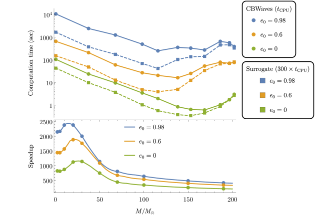
Fig. 10 shows (on top) the computation time or CPU time for CBwaves waveforms (solid lines) against corresponding surrogate waveforms (dashed lines) as a function of total mass of the binary system. The total mass $M$ is measured in the same 11 points as in Fig. 1 for three different initial eccentricities ($e_{0}=\{0.98,\,0.6,\,0\}$) of equal-mass configurations, each associated with different colours. The computation time $t_{\text{CPU}}$ for surrogates is multiplied by a factor of $300$ in order to shift the curves close to their respective CBwaves counterparts and enable visual comparison. The bottom panel demonstrates that surrogates are several thousand times faster around $10-50$ $M_{\odot}$ to evaluate as compared to the cost of generating CBwaves waveforms. The speedup falls off to several hundreds as the total mass increases. Moreover, the speedup grows when the initial eccentricity $e_{0}$ is increased in much the same way as with the mass disparity $\bar{q}$ (cf. Fig. 6 in Pürrer (2016)). The speedup is roughly twice as great for configurations having extremely high initial eccentricity ($e_{0}=0.98$) as for circular ones ($e_{0}=0$). The resemblance of the influence of $e_{0}$ and $\bar{q}$ exercize on the speedup can be attributed to their asymptotical nature as it had been pointed out earlier in Sec. II.1. It is also evident that the speedup culminates when waveforms for configurations of very low total mass and very high eccentricity are generated. Such waveforms are prohibitively expensive to generate with CBwaves in contrast to surrogates that are generated at the same cost, regardless of the parameters of the configuration.

Let us note that successive versions of SEOBNR ROMs have been developed and put to use within LAL (LSC Algorithms Library) to shorten data analysis applications carried out since the first observation runs have begun. Veitch et al. It has been shown in Field et al. (2014, 2011) that the cost of evaluating the surrogate model is linear in the number of samples $N$ (cf. our Fig. 8 where the surrogate error depends on the sampling rate). Depending on the sampling rate, the speedup is between 2 and almost 4 orders of magnitude. The speedup in evaluating surrogate models compared to generating NR waveforms with the LAL analysis routines is crucial for searches and theoretical parameter estimations. SEOBNR (aligned-spin Effective-One-Body), IMRPhenomD (Inspiral-Merger-Ringdown Phenomenological Model ‘D’) and PhenSpinTaylorRD waveform approximants are among the best available GW models for generic spinning, compact binaries. In comparison with our results, the speedup achieved at the typical rate of $2.048$ kHz used by aLIGO and aVirgo observatories is roughly $2300$. Aasi et al. (2013)