Fast solvers for the high-order FEM simplicial de Rham complex

Pablo D. Brubeck Mathematical Institute, University of Oxford, Oxford, UK brubeckmarti@maths.ox.ac.uk , Patrick E. Farrell Mathematical Institute, University of Oxford, Oxford, UK patrick.farrell@maths.ox.ac.uk , Robert C. Kirby Department of Mathematics, Baylor University, Waco, TX, US robert_kirby@baylor.edu and Charles Parker Ridgway Scott Foundation, 2544 S Forest Ln, Cedarville, MI charles_parker@alumni.brown.edu

(Date: September 28, 2025)

Abstract.

We present new finite elements for solving the Riesz maps of the de Rham complex on triangular and tetrahedral meshes at high order. The finite elements discretize the same spaces as usual, but with different basis functions, so that the resulting matrices have desirable properties. These properties mean that we can solve the Riesz maps to a given accuracy in a $p$ -robust number of iterations with $\mathcal{O}(p^{6})$ flops in three dimensions, rather than the naïve $\mathcal{O}(p^{9})$ flops.

The degrees of freedom build upon an idea of Demkowicz et al., and consist of integral moments on an equilateral reference simplex with respect to a numerically computed polynomial basis that is orthogonal in two different inner products. As a result, the interior-interface and interior-interior couplings are provably weak, and we devise a preconditioning strategy by neglecting them. The combination of this approach with a space decomposition method on vertex and edge star patches allows us to efficiently solve the canonical Riesz maps at high order. We apply this to solving the Hodge Laplacians of the de Rham complex with novel augmented Lagrangian preconditioners.

2020 Mathematics Subject Classification:

Primary 65F08, 65N35, 65N55

PBD was supported by EPSRC grant EP/W026260/1

PEF was supported by EPSRC grant EP/W026260/1, the Donatio Universitatis Carolinae Chair “Mathematical modelling of multicomponent systems”, and the UKRI Digital Research Infrastructure Programme through the Science and Technology Facilities Council’s Computational Science Centre for Research Communities (CoSeC)

CP acknowledges this material is based upon work supported by the National Science Foundation under Award No. DMS-2201487

1. Introduction

High-order finite element discretizations have very attractive properties, such as rapid convergence and high arithmetic intensity. However, their implementation requires great care, as naïve approaches to operator evaluation and linear system solution can scale badly in terms of memory and floating-point operations (flops) as the polynomial degree $p$ increases. On a single $d$ -dimensional cell, the number of degrees of freedom scales like $p^{d}$ ; computing the $\mathcal{O}(p^{2d})$ entries of a dense stiffness matrix with standard Lagrange-type elements would cost $\mathcal{O}(p^{3d})$ flops. Making high-order discretizations competitive therefore requires better algorithms.

For tensor-product cells (quadrilaterals and hexahedra), a tensor-product basis naturally exposes the required structure to decouple multidimensional problems into a sequence of one-dimensional problems, reducing computational cost and storage. For example, the sum-factorization assembly strategy enables fast matrix-free operator evaluation in $\mathcal{O}(p^{d+1})$ operations and $\mathcal{O}(p^{d})$ storage [42], and the fast diagonalization method (FDM) addresses the solution of separable problems on structured domains with the same complexities [36]. The previous work of the first two authors employing FDM-inspired finite element bases with suitable space decompositions yields the solution of certain separable and non-separable problems on unstructured domains with the same complexities [14, 15]. In particular, these complexities are achieved on tensor-product cells for the solution of the following partial differential equations (PDEs), posed on a bounded Lipschitz domain $\Omega\subset\mathbb{R}^{d}$ with $d=3$ for concreteness:

(1.1)	$\displaystyle\beta u-\nabla\cdot\left(\alpha\nabla u\right)$	$\displaystyle=f\mbox{\leavevmode\nobreak\ in\leavevmode\nobreak\ }\Omega,\quad$	$\displaystyle u$	$\displaystyle=0\mbox{\leavevmode\nobreak\ on\leavevmode\nobreak\ }\Gamma_{D},\quad$	$\displaystyle\alpha\nabla u\cdot\mathbf{n}$	$\displaystyle=0\text{\leavevmode\nobreak\ on\leavevmode\nobreak\ }\Gamma_{N};$
(1.2)	$\displaystyle\beta\mathbf{u}+\nabla\times\left(\alpha\nabla\times\mathbf{u}\right)$	$\displaystyle=\mathbf{f}\mbox{\leavevmode\nobreak\ in\leavevmode\nobreak\ }\Omega,$	$\displaystyle\mathbf{u}\times\mathbf{n}$	$\displaystyle=0\mbox{\leavevmode\nobreak\ on\leavevmode\nobreak\ }\Gamma_{D},\quad$	$\displaystyle\alpha\nabla\times\mathbf{u}\times\mathbf{n}$	$\displaystyle=0\text{\leavevmode\nobreak\ on\leavevmode\nobreak\ }\Gamma_{N};$
(1.3)	$\displaystyle\beta\mathbf{u}-\nabla\left(\alpha\nabla\cdot\mathbf{u}\right)$	$\displaystyle=\mathbf{f}\mbox{\leavevmode\nobreak\ in\leavevmode\nobreak\ }\Omega,\quad$	$\displaystyle\mathbf{u}\cdot\mathbf{n}$	$\displaystyle=0\mbox{\leavevmode\nobreak\ on\leavevmode\nobreak\ }\Gamma_{D},\quad$	$\displaystyle\alpha\nabla\cdot\mathbf{u}$	$\displaystyle=0\text{\leavevmode\nobreak\ on\leavevmode\nobreak\ }\Gamma_{N}.$

Here $\alpha,\beta:\Omega\to\mathbb{R}_{+}$ are given coefficients, $f:\Omega\to\mathbb{R}$ and $\mathbf{f}:\Omega\to\mathbb{R}^{3}$ are given source functions, $\Gamma_{D}\subseteq\partial\Omega$ , and $\Gamma_{N}=\partial\Omega\setminus\Gamma_{D}$ . For $\alpha=\beta=1$ , these equations are the so-called Riesz maps associated with subsets of the spaces $H(\operatorname{grad},\Omega)=H^{1}(\Omega)$ , $H(\operatorname{curl},\Omega)$ , and $H(\operatorname{div},\Omega)$ , respectively. For brevity we shall write $H(\operatorname{grad})=H(\operatorname{grad},\Omega)$ etc. where there is no potential confusion. These equations 1.1, 1.2 and 1.3 often arise as subproblems in the construction of preconditioners for more complex systems involving solution variables in $H(\operatorname{grad})$ , $H(\operatorname{curl})$ , and $H(\operatorname{div})$ [26, 31, 38, 37].

Achieving $\mathcal{O}(p^{d+1})$ operations and $\mathcal{O}(p^{d})$ storage on simplices is more challenging. Bases constructed from collapsed-coordinate mappings [30] give one possible approach, allowing a similar sum-factorization evaluation strategy. Perhaps surprisingly, Bernstein–Bézier expansions also admit sum-factorized matrix-free operator evaluation in $\mathcal{O}(p^{d+1})$ operations and $\mathcal{O}(p^{d})$ storage [1, 32], and such techniques have been generalized to the entire de Rham complex [2, 33]. For the $H(\operatorname{grad})$ mass matrix ( $\alpha=0$ ) in 2D, there are $\mathcal{O}(p^{3})$ solvers available [3]. However, there is no known solver for the linear systems arising from FEM discretizations of 1.1, 1.2 and 1.3 with these complexities. This manuscript makes a step towards addressing this challenge.

The essential idea of our approach is to devise new finite elements for the $L^{2}$ de Rham complex with favorable properties for solvers. With the basis functions we propose, the interior and interface degrees of freedom are provably weakly coupled. This motivates the use of block preconditioning strategies that decouple the interface and interior degrees of freedom. The degrees of freedom yielding this weak coupling are designed within the framework of Demkowicz et al. [18], by making a clever choice for bases of bubble spaces that arise in the construction of the degrees of freedom. These bases for the bubble spaces are constructed by solving a handful of offline eigenproblems on the reference cell for each polynomial degree $p$ . This combination of finite elements and block preconditioning strategy solves the Riesz maps of the $L^{2}$ de Rham complex in $\mathcal{O}(p^{3(d-1)})$ operations and $\mathcal{O}(p^{2(d-1)})$ storage, worse than the optimal complexities achieved on tensor-product cells, but orders better than the naïve approach. This is borne out in numerical experiments, as shown in Figure 1.

(a)

(b)

(c)

(d)

(e)

(f)

(g)

(h)

(i)

Figure 1. Flop counts, peak memory usage, and nonzeros in the sparse matrices and patch factors in the solution of the Riesz maps (

\alpha=\beta=1

) on a Freudenthal mesh with 3 cells in each direction.

Several other works have addressed the same problem of solving the Riesz maps at high order. For 1.1, Šolín and Vejchodský [50] introduced the idea of using generalized eigenfunctions as interior basis functions, which we also employ in our construction, but they do not address how to construct efficient solvers. Also for 1.1, Casarin and Sherwin [49] constructed nonoverlapping Schwarz methods for the Schur complement system requiring exact interior solves; however, these interior solves require $\mathcal{O}(p^{3d})$ operations. Low-order refined preconditioning is provably effective on tensor-product cells [44], but the extension to simplicial cells is delicate and has only been studied for 1.1 on triangles [16]. Beuchler and coauthors construct sparse hierarchical bases for discretizations of the de Rham complex using Jacobi polynomials [7, 8, 9, 10]; this approach yields sparser matrices than ours, but the bases here concentrate the nonzero entries in the interface block, enabling the efficient interior-interface space decomposition described in Theorem 6.1 below.

A disadvantage of our approach is that the resulting preconditioners are not parameter-robust in $\alpha$ and $\beta$ . We design elements suitable for the stiffness-dominated case, so that the preconditioner is provably robust for $\beta/\alpha\in[0,1)$ . This is the more difficult case of wider interest (e.g. arising in augmented Lagrangian preconditioning). We anticipate that it is possible to design a basis for the mass-dominated case ( $\beta/\alpha\gg 1$ ), but with very different properties.

2. Finite element discretization

Let $\Omega\subset\mathbb{R}^{d}$ be a bounded Lipschitz domain with boundary $\Gamma\coloneqq\partial\Omega$ . We denote the spaces consisting of $k$ -forms as $H(\operatorname{d}^{k},\Omega)=\{v\in L^{2}(\Omega):\operatorname{d}^{k}v\in L^{2}(\Omega)\}$ , where $\operatorname{d}^{k}$ denotes the exterior derivative on $k$ -forms ( $\operatorname{d}^{0}=\operatorname{grad}$ , $\operatorname{d}^{1}=\operatorname{curl}$ , $\operatorname{d}^{2}=\operatorname{div}$ , and $\operatorname{d}^{3}=0$ ). The trace operator on theses spaces $\operatorname{tr}^{k}_{\Gamma}:H(\operatorname{d}^{k},\Omega)\to H^{-1/2}(\Gamma)$ is defined by

(2.1)

\operatorname{tr}^{k}_{\Gamma}v\coloneqq\begin{cases}v|_{\Gamma}&\text{if }k=0,\\ \Pi_{\Gamma}v|_{\Gamma}&\text{if }k=1,\\ \mathbf{n}\cdot v|_{\Gamma}&\text{if }k=2,\end{cases}

where $\Pi_{\Gamma}$ denotes the projection of a vector onto the tangent space of $\Gamma$ . The trace operator is continuous, but not surjective if $k<2$ [12].

On a shape-regular, conforming simplicial mesh of $\Omega$ , denoted by $\mathcal{T}_{h}$ , we consider well-known finite element subcomplexes of the $L^{2}$ de Rham complex. For concreteness, we will restrict our discussion to the case $d=3$ :

Figure 2. The

L^{2}

de Rham complex in three dimensions (middle), and the finite element subcomplexes of the first (above) and second (below) kinds.

The top and bottom row of Figure 2 correspond to the subcomplexes of first and second kinds, respectively. In particular, $\mathrm{CG}_{p}$ and $\mathrm{DG}_{p}$ denote the usual spaces of continuous and discontinuous piecewise polynomials, $\mathrm{Ned}^{1}_{p}$ [40] and $\mathrm{Ned}^{2}_{p}$ [41] correspond to the $H(\operatorname{curl})$ -conforming spaces of the first and second kinds, and $\mathrm{RT}_{p}$ [45, 40] and $\mathrm{BDM}_{p}$ [13, 41] correspond to the $H(\operatorname{div})$ -conforming spaces of the first and second kinds. One can also form a hybrid complex by interchanging kinds as in Figure 3:

Figure 3. Hybrid subcomplexes of the

L^{2}

de Rham complex.

To unify our discussion, we employ the same notation $X^{k}_{p}(\hat{T})$ to denote the discrete spaces of $k$ -forms of the first or second kind on a reference equilateral simplex $\hat{T}$ . Here, $p$ denotes the degree of the polynomial spaces. In particular, for the first kind, we have

(2.2)

X^{k}_{p}(\hat{T})\coloneqq\left\{\begin{array}[]{rlll}\mathrm{CG}_{p}(\hat{T})&\coloneqq&\mathrm{P}_{p}(\hat{T})&\text{if }k=0,\\ \mathrm{Ned}^{1}_{p}(\hat{T})&\coloneqq&\mathrm{P}_{p-1}(\hat{T})^{3}+\mathrm{P}_{p-1}(\hat{T})^{3}\times\mathbf{x}&\text{if }k=1,\\ \mathrm{RT}_{p}(\hat{T})&\coloneqq&\mathrm{P}_{p-1}(\hat{T})^{3}+\mathrm{P}_{p-1}(\hat{T})\mathbf{x}&\text{if }k=2,\\ \mathrm{DG}_{p}(\hat{T})&\coloneqq&\mathrm{P}_{p}(\hat{T})&\text{if }k=3,\end{array}\right.

while for the second kind we have

(2.3)

X^{k}_{p}(\hat{T})\coloneqq\left\{\begin{array}[]{rlll}\mathrm{CG}_{p}(\hat{T})&\coloneqq&\mathrm{P}_{p}(\hat{T})&\text{if }k=0,\\ \mathrm{Ned}^{2}_{p}(\hat{T})&\coloneqq&\mathrm{P}_{p}(\hat{T})^{3}&\text{if }k=1,\\ \mathrm{BDM}_{p}(\hat{T})&\coloneqq&\mathrm{P}_{p}(\hat{T})^{3}&\text{if }k=2,\\ \mathrm{DG}_{p}(\hat{T})&\coloneqq&\mathrm{P}_{p}(\hat{T})&\text{if }k=3.\end{array}\right.

We define the global finite element space $X^{k}_{p}(\mathcal{T}_{h})$ in terms of the space on the reference cell $X^{k}_{p}(\hat{T})$ via the standard pullback:

(2.4)

X^{k}_{p}(\mathcal{T}_{h})\coloneqq\{v\in H(\operatorname{d}^{k},\Omega):\operatorname{\forall}T\in\mathcal{T}_{h}\ \operatorname{\exists}\hat{v}\in X^{k}_{p}(\hat{T})\text{ s.t.}\left.v\right|_{T}=\mathcal{F}^{k}_{T}(\hat{v})\},

where for a cell $T\in\mathcal{T}_{h}$ , the pullback $\mathcal{F}^{k}_{T}:H(\operatorname{d}^{k},\hat{T})\to H(\operatorname{d}^{k},T)$ is defined by:

(2.5)

\mathcal{F}^{k}_{T}(\hat{v})\coloneqq\begin{cases}\hat{v}\circ F_{T}^{-1}&\text{if }k=0,\\ J_{T}^{-\top}\hat{v}\circ F_{T}^{-1}&\text{if }k=1,\\ (\det J_{T})^{-1}J_{T}\hat{v}\circ F_{T}^{-1}&\text{if }k=2,\\ (\det J_{T})^{-1}\hat{v}\circ F_{T}^{-1}&\text{if }k=3,\end{cases}

where $F_{T}:\hat{T}\to T$ is a fixed bijective mapping from the reference cell $\hat{T}$ to the physical cell $T$ and $J_{T}$ denotes its Jacobian matrix. Denoting by $\Delta_{l}(\mathcal{T}_{h})$ the set of $l$ -dimensional subsimplices of $\mathcal{T}_{h}$ , we note that a discrete $k$ -form $v\in X^{k}_{p}(\mathcal{T}_{h})$ and any subset $S\subset\Delta_{l}(\mathcal{T}_{h})$ with $l=k:d-1$ , the trace $\operatorname{tr}^{k}_{S}v$ , given by formula 2.1 with $\Gamma$ replaced by $S$ is well-defined (see e.g. [6, Lemma 5.1]). We also define the trivial trace $\operatorname{tr}^{k}_{S}$ for a $d$ -dimensional subset $S\subset\mathcal{T}_{h}$ by $\operatorname{tr}^{k}_{S}v=v|_{S}$ .

With these spaces, the discrete weak formulation of problems 1.1, 1.2 and 1.3 is to find $u\in X^{k}_{p,D}(\mathcal{T}_{h})$ such that

(2.6)

a^{k}(u,v)\coloneqq(u,\beta v)+(\operatorname{d}^{k}u,\alpha\operatorname{d}^{k}v)=F(v)\qquad\operatorname{\forall}v\in X^{k}_{p,D}(\mathcal{T}_{h}),

where $X^{k}_{p,D}(\mathcal{T}_{h})$ is the subset of $X^{k}_{p}(\mathcal{T}_{h})$ with zero trace on $\Gamma_{D}$ :

(2.7)

X^{k}_{p,D}(\mathcal{T}_{h})\coloneqq\{u\in X^{k}_{p}(\mathcal{T}_{h}):\operatorname{tr}_{\Gamma_{D}}^{k}u=0\}.

For standard bases for $X^{k}_{p,D}(\mathcal{T}_{h})$ , the matrix corresponding to 2.6 will have dense $\mathcal{O}(p^{d})\times\mathcal{O}(p^{d})$ blocks.

3. Orthogonality-promoting discretizations

We wish to construct bases for $X^{k}_{p}(\mathcal{T}_{h})$ that enable fast solvers for problem 2.6 at high order. In particular, we wish to promote orthogonality of the basis in the $L^{2}$ and $H(\operatorname{d}^{k})$ inner products. However, constructing such bases would involve the solution of global eigenproblems, which is not appealing. Instead, we devise bases so that the interior basis functions are orthogonal in these inner products on the reference cell. This will ensure that the interior-interior block of the mass and stiffness matrices associated with the $L^{2}(\hat{T})$ and $H(\operatorname{d}^{k},\hat{T})$ inner products are diagonal on the reference cell.

To form bases with this interior orthogonality property, we follow the definition of interpolation degrees of freedom from Demkowicz et al. [18]. Demkowicz et al. employed these degrees of freedom to define interpolation operators with commuting diagram properties; here, we will use them to define finite elements, through the Ciarlet dual basis construction [17]. In particular, given a set of degrees of freedom $\{\ell_{j}\}$ , the basis $\{\phi_{j}\}$ is constructed so that $\ell_{j}(\phi_{i})=\delta_{ij}$ .

For the remainder of the manuscript, we select one of the discrete subcomplexes in Figures 2 and 3 and drop the subscript “ $p$ ” so that the complexes read

(3.1)

In particular, $X^{k}(\hat{T})$ may be a first or second kind space provided that 3.1 is exact. Although we will first proceed in this abstract setting, the degrees of freedom for each of the spaces in 2.2 and 2.3 and the corresponding spaces in 2D are listed explicitly in section 3.4.

3.1. Degrees of freedom with commuting diagram properties

Let $k\in 0:d-1$ be fixed. The bubble spaces on a cell subentity $S\in\Delta_{l}(\hat{T})$ with $l\in k+1:d$ , which play a key role in the degrees of freedom in [18], are defined by

(3.2)

\mathring{X}^{k}(S)\coloneqq\left\{\operatorname{tr}_{S}^{k}v:v\in X^{k}(\hat{T})\text{ and }\operatorname{tr}_{\partial S}^{k}v=0\right\}.

We will later construct bases for these bubble spaces so as to promote sparsity. We also define differential operators on the trace subspace $\operatorname{tr}_{S}^{k}X^{k}(\hat{T})$ for $S\in\Delta_{l}(\hat{T})$ with $l\in k+1:d-1$ , as follows:

(3.3)

\displaystyle\operatorname{d}_{S}^{0}v

\displaystyle\coloneqq\operatorname{grad}_{S}v\quad\text{and}\quad\operatorname{d}_{S}^{1}v\coloneqq\operatorname{curl}_{S}v,

where $\operatorname{grad}_{S}$ denotes the tangential surface gradient taking values in $\mathbb{R}^{l}$ and $\operatorname{curl}_{S}$ is the surface curl/rot operator taking values in $\mathbb{R}$ . Crucially, these operators are defined so that

(3.4)

\displaystyle\operatorname{d}_{S}^{k}\operatorname{tr}_{S}^{k}v

\displaystyle=\operatorname{tr}_{S}^{k+1}\operatorname{d}^{k}v\qquad

\displaystyle\operatorname{\forall}v\in X^{k}(\hat{T}).

The commuting interpolation procedure given in [18, 53] is based on the following linear functionals


(3.5a)	$\displaystyle(q,\operatorname{tr}^{k}_{S}v)_{S},\qquad$	$\displaystyle\operatorname{\forall}S\in\Delta_{k}(\hat{T}),\$	$\displaystyle\operatorname{\forall}q\in\operatorname{tr}^{k}_{S}X^{k}(\hat{T}),$
(3.5b)	$\displaystyle(\operatorname{d}_{S}^{k}q,\operatorname{d}^{k}_{S}\operatorname{tr}^{k}_{S}v)_{S}\qquad$	$\displaystyle\operatorname{\forall}S\in\bigcup_{l=k+1}^{d}\Delta_{l}(\hat{T}),\$	$\displaystyle\operatorname{\forall}q\in\mathring{X}^{k}(S),$
(3.5c)	$\displaystyle(\operatorname{d}_{S}^{k-1}q,\operatorname{tr}^{k}_{S}v)_{S}\qquad$	$\displaystyle\operatorname{\forall}S\in\bigcup_{l=k+1}^{d}\Delta_{l}(\hat{T}),\$	$\displaystyle\operatorname{\forall}q\in\mathring{X}^{k-1}(S),$

which we will use to construct a set of degrees of freedom by fixing bases for each of the subspaces above.

3.2. Local space decomposition

We observe that in the linear functionals 3.5b and 3.5c, only $\operatorname{d}^{k}_{S}q$ and $\operatorname{d}^{k-1}_{S}q$ appear, and so the construction of a unisolvent set of degrees of freedom requires finding minimal sets $\{q\}$ such that $\{\operatorname{d}^{k}_{S}q\}$ forms a basis for $\operatorname{d}^{k}_{S}\mathring{X}^{k}(S)$ . Since $\operatorname{d}^{k}_{S}$ may have a nontrivial kernel, it will be convenient to characterize this kernel. This characterization can be readily achieved by considering the bubble subcomplex for $S\in\Delta_{l}(\hat{T})$ with $l\in k+1:d$ :

(3.6)

We define the subspaces


(3.7a)	$\displaystyle\mathring{X}^{k,\mathrm{I}}(S)$	$\displaystyle\coloneqq\left\{v\in\mathring{X}^{k}(S):(v,w)_{S}=0\ \operatorname{\forall}w\in\ker(\operatorname{d}_{S}^{k};\mathring{X}^{k})\right\},$
(3.7b)	$\displaystyle\mathring{X}^{k,\mathrm{II}}(S)$	$\displaystyle\coloneqq\ker(\operatorname{d}_{S}^{k};\mathring{X}^{k}),$

Since the complex 3.6 is exact thanks to Lemma A.1, the kernel of $\operatorname{d}_{S}^{k}$ acting on $\mathring{X}^{k}(S)$ is simply $\operatorname{d}^{k-1}_{S}\mathring{X}^{k-1}(S)$ and so $\mathring{X}^{k,\mathrm{II}}(S)=\operatorname{d}^{k-1}_{S}\mathring{X}^{k-1}(S)$ . In particular, we have the following $L^{2}(S)$ -orthogonal decomposition:

(3.8)

\mathring{X}^{k}(S)=\mathring{X}^{k,\mathrm{I}}(S)\oplus\mathring{X}^{k,\mathrm{II}}(S)=\mathring{X}^{k,\mathrm{I}}(S)\oplus\operatorname{d}_{S}^{k-1}\mathring{X}^{k-1,\mathrm{I}}(S).

Therefore, we may select the functions in 3.5b and 3.5c from $\mathring{X}^{k,\mathrm{I}}(S)$ and $\mathring{X}^{k-1,\mathrm{I}}(S)$ , respectively.

We now perform a similar decomposition of the trace space $\operatorname{tr}^{k}_{S}X^{k}(\hat{T})$ , $S\in\Delta_{k}(\hat{T})$ , to select the functions in 3.5a. We adopt the convention that for $E\in\Delta_{1}(\hat{T})$ and $v\in X^{1}(\hat{T})$ , the projection onto the tangent space of $E$ is scalar-valued, and thus $\operatorname{tr}^{k}_{S}X^{k}(\hat{T})$ , $S\in\Delta_{k}(\hat{K})$ , is scalar-valued for $k\in 0:d-1$ . Thanks to Lemma A.2, we have the following $L^{2}(S)$ -orthogonal decomposition of the trace space $\operatorname{tr}^{k}_{S}X^{k}(\hat{T})$ :

(3.9)

\operatorname{tr}^{k}_{S}X^{k}(\hat{T})=\operatorname{tr}^{k}_{S}W^{k}(\hat{T})\oplus\operatorname{d}_{S}^{k-1}\mathring{X}^{k-1,\mathrm{I}}(S)=\mathbb{R}\oplus\operatorname{d}_{S}^{k-1}\mathring{X}^{k-1,\mathrm{I}}(S)

where $W^{k}(\hat{T})$ denotes the space of Whitney forms, defined as the lowest-order finite element space of the first kind; e.g., if $d=3$ , then

(3.10)

W^{k}(\hat{T})\coloneqq\begin{cases}\mathrm{CG}_{1}(\hat{T})&\text{if }k=0,\\ \mathrm{Ned}^{1}_{1}(\hat{T})&\text{if }k=1,\\ \mathrm{RT}_{1}(\hat{T})&\text{if }k=2,\\ \mathrm{DG}_{0}(\hat{T})&\text{if }k=3.\end{cases}

In contrast to [18], we further decompose 3.5a using 3.9 by choosing $q$ in 3.5a to be the constant 1 and of the form $\operatorname{d}_{S}^{k-1}\tilde{q}$ , where $\tilde{q}\in\mathring{X}^{k-1,\mathrm{I}}_{p}(S)$ . As we will see in Lemma 4.1, this choice ensures that the canonical basis for the Whitney forms is contained in the high-order basis. We will achieve an interior orthogonality property through a careful and novel choice of basis for the bubble spaces $\mathring{X}^{k,\mathrm{I}}(S)$ .

3.3. Abstract construction of orthogonality-promoting basis

We define the finite elements via a Ciarlet triple $(\hat{T},X^{k}(\hat{T}),\mathcal{L})$ , where the set $\mathcal{L}=\{\ell_{j}^{k}\}$ is a basis for the dual space $(X^{k}(\hat{T}))^{*}$ , with degrees of freedom $\ell_{j}^{k}$ that map a $k$ -form $v\in X^{k}(\hat{T})$ to a real number $\ell_{j}^{k}(v)$ . Let $N^{k}_{S}\coloneqq\dim\mathring{X}^{k,\mathrm{I}}(S)$ denote the dimension of the type- $\mathrm{I}$ bubble spaces for $S\in\Delta_{l}(\hat{T})$ , $l\in k+1:d$ . For notational convenience, we also define $N^{k}_{S}\coloneqq\dim\operatorname{tr}^{k}_{S}W^{k}(\hat{T})=1$ for $S\in\Delta_{k}(\hat{T})$ . Thanks to 3.8 and 3.9, there holds


(3.11a)	$\displaystyle\dim\mathring{X}^{k}(S)$	$\displaystyle=N^{k}_{S}+N^{k-1}_{S}\qquad$	$\displaystyle\operatorname{\forall}S\in\bigcup_{l=k+1}^{d}\Delta_{l}(\hat{T}),$
(3.11b)	$\displaystyle\dim\operatorname{tr}_{S}^{k}X^{k}(\hat{T})$	$\displaystyle=1+N^{k-1}_{S}\qquad$	$\displaystyle\operatorname{\forall}S\in\Delta_{k}(\hat{T}).$

For $k\in 0:d-1$ and $l\in k+1:d$ and each subsimplex $S\in\Delta_{l}(\hat{T})$ , we compute an eigenbasis of the bubbles $\{\psi_{S,j}^{k}:j\in 1:N^{k}_{S}\}\subseteq\mathring{X}^{k,\mathrm{I}}(S)$ that solves the following eigenvalue problem:

(3.12)

(\operatorname{d}_{S}^{k}\psi_{S,j}^{k},\operatorname{d}_{S}^{k}\psi_{S,i}^{k})_{S}=\delta_{ij}\quad\text{and}\quad(\psi_{S,j}^{k},\psi_{S,i}^{k})_{S}=\lambda_{S,j}\delta_{ij}\qquad\operatorname{\forall}\leavevmode\nobreak\ i,j\in 1:N^{k}_{S}.

The eigenbases $\{\psi_{S,j}^{k}\}$ are numerically computed offline and only once for each relevant reference subsimplex. Then, by construction, the set $\{\psi_{S,j}^{k}\}$ forms a basis for $\mathring{X}^{k,\mathrm{I}}(S)$ , and the set $\{\operatorname{d}_{S}^{k}\psi_{S,j}^{k}\}$ forms a basis for $\operatorname{d}_{S}^{k}\mathring{X}^{k}(S)$ .

Here, we choose $\hat{T}$ to be an equilateral simplex so that only one facet, edge, etc. needs to be computed, and the rest are constructed by the appropriate pullback. We compute the solution to 3.12 by first solving the following augmented eigenvalue problem on the whole bubble space $\mathring{X}^{k}$ :

(3.13)

(\operatorname{d}_{S}^{k}\hat{\psi}_{S,j}^{k},\operatorname{d}_{S}^{k}\hat{\psi}_{S,i}^{k})_{S}=\mu_{S,j}\delta_{ij}\quad\text{and}\quad(\hat{\psi}_{S,j}^{k},\hat{\psi}_{S,i}^{k})_{S}=\delta_{ij}\qquad\operatorname{\forall}\leavevmode\nobreak\ i,j\in 1:\dim\mathring{X}^{k}.

Then, we renormalize the subset of eigenfunctions for which $\mu_{S,j}\neq 0$ to form the solution to 3.12.

Our degrees of freedom for the discrete spaces in the $L^{2}$ -de Rham complex $X^{k}(\hat{T})$ are defined as follows. On each subsimplex we prescribe two types of degrees of freedom if $k>0$ . On each $k$ -simplex $S\in\Delta_{k}(\hat{T})$ , we augment the degrees of freedom for Whitney forms 3.14a with integral moments against the exterior derivative of the basis for the bubble space of $(k-1)$ -forms $\mathring{X}^{k-1}(S)$ . On the remaining sub-simplices of dimension $l\in k+1:d$ , $S\in\Delta_{l}(\hat{T})$ , we prescribe integral moments of $\operatorname{d}^{k}_{S}\operatorname{tr}^{k}_{S}v$ against the eigenbasis for $\operatorname{d}^{k}_{S}\mathring{X}^{k}$ , and integral moments of $\operatorname{tr}^{k}_{S}v$ against the eigenbasis for $\operatorname{d}^{k-1}_{S}\mathring{X}^{k-1}(S)$ :


(3.14a)	$\displaystyle\ell^{k,\mathrm{I}}_{S,1}(v)$	$\displaystyle\coloneqq(1,\operatorname{tr}^{k}_{S}v)_{S},\qquad$	$\displaystyle\operatorname{\forall}S\in\Delta_{k}(\hat{T}),$
(3.14b)	$\displaystyle\ell^{k,\mathrm{I}}_{S,j}(v)$	$\displaystyle\coloneqq(\operatorname{d}_{S}^{k}\psi_{S,j}^{k},\operatorname{d}_{S}^{k}\operatorname{tr}^{k}_{S}v)_{S}\qquad$	$\displaystyle\operatorname{\forall}S\in\bigcup_{l=k+1}^{d}\Delta_{l}(\hat{T}),\ \operatorname{\forall}j\in 1:N^{k}_{S},$
(3.14c)	$\displaystyle\ell^{k,\mathrm{II}}_{S,j}(v)$	$\displaystyle\coloneqq(\operatorname{d}_{S}^{k-1}\psi_{S,j}^{k-1},\operatorname{tr}^{k}_{S}v)_{S}\qquad$	$\displaystyle\operatorname{\forall}S\in\bigcup_{l=k}^{d}\Delta_{l}(\hat{T}),\ \operatorname{\forall}j\in 1:N^{k-1}_{S}.$

We collect the degrees of freedom into a single set

(3.15)

\mathcal{L}:=\bigcup_{l=k}^{d}\bigcup_{S\in\Delta_{l}(\hat{T})}\{\ell^{k,\mathrm{I}}_{S,j}:j\in 1:N^{k}_{S}\}\cup\{\ell^{k,\mathrm{II}}_{S,j}:j\in 1:N^{k-1}_{S}\}.

The unisolvence of the degrees of freedom $\mathcal{L}$ follows from standard arguments.

Lemma 3.1.

The degrees of freedom 3.15 are unisolvent on $X^{k}(\hat{T})$ .

Proof.

We first show that $\dim\mathcal{L}=\dim X^{k}(\hat{T})$ . Note that

	$\displaystyle\dim\mathcal{L}$	$\displaystyle=\sum_{S\in\Delta_{k}(\hat{T})}\left(1+N_{S}^{k-1}\right)+\sum_{l=k+1}^{d}\sum_{S\in\Delta_{l}(\hat{T})}\left(N_{S}^{k}+N_{S}^{k-1}\right)$
		$\displaystyle=\sum_{S\in\Delta_{k}(\hat{T})}\dim\operatorname{tr}_{S}^{k}X^{k}(\hat{T})+\sum_{l=k+1}^{d}\sum_{S\in\Delta_{l}(\hat{T})}\dim\mathring{X}^{k}(S),$

where we used 3.11. Thanks to [5, Theorem 5.5 & Lemma 5.6], we conclude that $\dim\mathcal{L}=\dim X^{k}(\hat{T})$ .

Now suppose that $v\in X^{k}(\hat{T})$ satisfies $\ell(v)=0$ for all $\ell\in\mathcal{L}$ . Since 3.14a vanishes, the decomposition 3.9 shows that for all $S\in\Delta_{k}(\hat{T})$ , $\operatorname{tr}_{S}^{k}v=\operatorname{d}_{S}^{k-1}w_{S}$ for some $w_{S}\in\mathring{X}^{k-1,\mathrm{I}}(S)$ . However, the degrees of freedom 3.14c vanish, and so $\operatorname{tr}_{S}^{k}v\equiv 0$ .

We may now proceed inductively on $l\in k+1:d$ . For $S\in\Delta_{l}(\hat{T})$ with $l\in k+1:d$ , $\operatorname{tr}_{S}^{k}v\in\mathring{X}^{k}(S)$ , and so $\operatorname{d}_{S}^{k}\operatorname{tr}_{S}^{k}v\equiv 0$ by 3.14b. By the exactness of 3.6, $\operatorname{tr}_{S}^{k}v=\operatorname{d}_{S}^{k-1}w_{S}$ for some $w_{S}\in\mathring{X}^{k-1,\mathrm{I}}(S)$ . The degrees of freedom 3.14c then give $w_{S}\equiv 0$ . Since this holds with $S=\hat{T}$ , $v\equiv 0$ . The unisolvence of $\mathcal{L}$ now follows. ∎

3.4. Concrete definition of orthogonality-promoting degrees of freedom

For the sake of readability, we have simplified our notation slightly by dropping the $k$ -form superscript and explicitly writing out the trace operators.

3.4.1. Degrees of freedom for $H(\operatorname{grad})$

We discretize $H(\operatorname{grad},\hat{T})$ with the space $\mathrm{CG}_{p}(\hat{T})$ . For each subsimplex $S\in\Delta_{l}(\hat{T})$ with $l\in 1:d$ , we compute the eigenbasis $\{\psi_{S,j}\}$ for $\mathring{X}^{0,\mathrm{I}}(S)=\mathring{X}^{0}(S)$ satisfying

(3.16)

(\operatorname{grad}_{S}\psi_{S,j},\operatorname{grad}_{S}\psi_{S,i})_{S}=\delta_{ij},\quad(\psi_{S,j},\psi_{S,i})_{S}=\lambda_{j}\delta_{ij},

where we recall that $\operatorname{grad}_{S}$ is the tangential gradient on $S$ . The degrees of freedom for $X^{0}(\hat{T})$ in 3.15 are point evaluations at vertices and integral moments of surface gradients on each higher-dimensional subsimplex:


(3.17a)	$\displaystyle\ell_{V}(v)$	$\displaystyle=v(V)\qquad$	$\displaystyle\operatorname{\forall}V\in\Delta_{0}(\hat{T}),$
(3.17b)	$\displaystyle\ell_{S,j}(v)$	$\displaystyle=(\operatorname{grad}_{S}\psi_{S,j},\operatorname{grad}_{S}v)_{S}\qquad$	$\displaystyle\operatorname{\forall}S\in\bigcup_{l=1}^{d}\Delta_{l}(\hat{T}).$

3.4.2. Degrees of freedom for $H(\operatorname{curl})$

We discretize $H(\operatorname{curl},\hat{T})$ with $X^{1}(\hat{T})$ , which we recall is either $\mathrm{Ned}^{1}_{p}(\hat{T})$ or $\mathrm{Ned}^{2}_{p}(\hat{T})$ , so that the corresponding space $X^{0}(\hat{T})$ is either $\mathrm{CG}_{p}(\hat{T})$ or $\mathrm{CG}_{p+1}(\hat{T})$ , respectively. We define a basis for the dual of $X^{1}(\hat{T})$ by using the eigenbasis $\{\psi_{S,j}\}$ constructed in 3.16 for the $H(\operatorname{grad})$ bubbles $\mathring{X}^{0}(S)$ . For each subsimplex $S\in\Delta_{l}(\hat{T})$ with $l\in 2:d$ , we compute the eigenbasis $\{\Psi_{S,j}\}$ for $\mathring{X}^{1,\mathrm{I}}(S)$ satisfying

(3.18)

(\operatorname{curl}_{S}\Psi_{S,j},\operatorname{curl}_{S}\Psi_{S,i})_{S}=\delta_{ij},\quad(\Psi_{S,j},\Psi_{S,i})_{S}=\lambda_{j}\delta_{ij},

where we recall that $\operatorname{curl}_{S}$ is the tangential curl on $S$ . As mentioned above, $\{\operatorname{curl}_{S}\Psi_{S,j}\}$ is a basis for $\operatorname{curl}_{S}\mathring{X}^{1}(S)$ .

The degrees of freedom for $X^{1}(\hat{T})$ in 3.15 are tangential moments along edges, moments of curl against curls and moments against gradients on each higher-dimensional subsimplex:


(3.19a)	$\displaystyle\ell^{\mathrm{I}}_{E,1}(v)$	$\displaystyle=(1,\mathbf{t}\cdot v)_{E}\qquad$	$\displaystyle\operatorname{\forall}E\in\Delta_{1}(\hat{T}),$
(3.19b)	$\displaystyle\ell^{\mathrm{I}}_{S,j}(v)$	$\displaystyle=(\operatorname{curl}_{S}\Psi_{S,j},\operatorname{curl}_{S}\Pi_{S}v)_{S}\qquad$	$\displaystyle\operatorname{\forall}S\in\bigcup_{l=2}^{d}\Delta_{l}(\hat{T}),$
(3.19c)	$\displaystyle\ell^{\mathrm{II}}_{S,j}(v)$	$\displaystyle=(\operatorname{grad}_{S}\psi_{S,j},\Pi_{S}v)_{S}\qquad$	$\displaystyle\operatorname{\forall}S\in\bigcup_{l=1}^{d}\Delta_{l}(\hat{T}),$

where we recall that $\Pi_{S}$ is the projection operator onto the tangent space of $S$ . In particular, the only difference between $\mathrm{Ned}^{1}_{p}(\hat{T})$ and $\mathrm{Ned}^{2}_{p}(\hat{T})$ is in 3.19c. For $\mathrm{Ned}^{1}_{p}(\hat{T})$ , the eigenfunctions $\psi_{S,j}$ defined in 3.16 and appearing in 3.19c are degree $p$ , while for $\mathrm{Ned}^{2}_{p}(\hat{T})$ , they are degree $p+1$ .

3.4.3. Degrees of freedom for $H(\operatorname{div})$

We discretize $H(\operatorname{div},\hat{T})$ with $X^{2}(\hat{T})$ , which we recall is either $\mathrm{RT}_{p}(\hat{T})$ or $\mathrm{BDM}_{p}(\hat{T})$ . If $X^{2}(\hat{T})=\mathrm{RT}_{p}(\hat{T})$ , then we can choose $X^{1}(\hat{T})$ as either $\mathrm{Ned}^{1}_{p}$ or $\mathrm{Ned}^{2}_{p}$ , while if $X^{2}(\hat{T})=\mathrm{BDM}_{p}(\hat{T})$ , we can choose $X^{1}_{p}(\hat{T})$ as either $\mathrm{Ned}^{1}_{p+1}$ or $\mathrm{Ned}^{2}_{p+1}$ . The resulting basis will depend on this particular choice, but the properties of the basis in the remainder of the manuscript are independent of this choice. For the implementation, we always choose $X^{1}(\hat{T})$ to be the corresponding space of the second kind.

We define a basis for the dual of $X^{2}(\hat{T})$ by using the eigenbasis $\{\Psi_{F,j}\}$ constructed in 3.18 for the $H(\operatorname{curl})$ bubbles $\mathring{X}^{1,\mathrm{I}}(F)$ . On the interior of $\hat{T}$ , we compute the eigenbasis $\{\Phi_{C,j}\}$ for $\mathring{X}^{2,\mathrm{I}}(\hat{T})$ satisfying

(3.20)

(\operatorname{div}\Phi_{C,j},\operatorname{div}\Phi_{C,i})_{\hat{T}}=\delta_{ij},\quad(\Phi_{C,j},\Phi_{C,i})_{\hat{T}}=\lambda_{j}\delta_{ij}.

As mentioned above, $\{\operatorname{div}\Psi_{C,j}\}$ is a basis for $\operatorname{div}\mathring{X}^{2}(\hat{T})$ .

The degrees of freedom for $X^{2}(\hat{T})$ in 3.15 are normal moments on faces, moments of divergence against divergences and moments against curls:


(3.21a)	$\displaystyle\ell^{\mathrm{I}}_{F,1}(v)$	$\displaystyle=(1,\mathbf{n}\cdot v)_{F}\qquad$	$\displaystyle\operatorname{\forall}F\in\Delta_{d-1}(\hat{T}),$
(3.21b)	$\displaystyle\ell^{\mathrm{II}}_{F,j}(v)$	$\displaystyle=(\operatorname{curl}_{F}\Psi_{F,j},\mathbf{n}\cdot v)_{F},\qquad$	$\displaystyle\operatorname{\forall}F\in\Delta_{d-1}(\hat{T}),$
(3.21c)	$\displaystyle\ell^{\mathrm{I}}_{C,j}(v)$	$\displaystyle=(\operatorname{div}\Phi_{C,j},\operatorname{div}v)_{\hat{T}},\qquad$
(3.21d)	$\displaystyle\ell^{\mathrm{II}}_{C,j}(v)$	$\displaystyle=(\operatorname{curl}\Psi_{C,j},v)_{\hat{T}}.$

Note that the only difference between $\mathrm{RT}_{p}(\hat{T})$ or $\mathrm{BDM}_{p}(\hat{T})$ are the eigenfunctions $\Psi_{F,j}$ and $\Psi_{C,j}$ defined in 3.18 appearing in 3.21b and 3.21d. For $\mathrm{RT}_{p}(\hat{T})$ , these eigenfunctions are $\mathrm{Ned}^{1}_{p}$ or $\mathrm{Ned}^{2}_{p}$ functions (or their trace), while for $\mathrm{BDM}_{p}(\hat{T})$ , they are $\mathrm{Ned}^{1}_{p+1}(\hat{T})$ or $\mathrm{Ned}^{2}_{p+1}(\hat{T})$ functions (or their trace).

Remark 3.2.

The degrees of freedom in 3.17 and 3.19 for discretizations of $H(\operatorname{grad})$ and $H(\operatorname{curl})$ are well-defined for $d=2$ . To discretize $H(\operatorname{div})$ in 2D, which corresponds to $k=1$ , we choose $X^{0}(\hat{T})$ to be $\mathrm{CG}_{p}$ if $X^{1}(\hat{T})=\mathrm{RT}_{p}$ or $\mathrm{CG}_{p+1}$ if $X^{1}(\hat{T})=\mathrm{BDM}_{p}$ and the operator $\operatorname{curl}_{F}$ in 3.21b is the tangential derivative operator and $\operatorname{curl}$ in 3.21d corresponds to a $\pi/2$ rotation of the gradient operator.

4. Properties of the basis on the reference cell

For $k\in 0:d-1$ , let

(4.1)

\displaystyle\left\{\phi_{S,j}^{k,\mathrm{I}},\phi_{S,n}^{k,\mathrm{II}}:j=1:N^{k}_{S},\ n=1:N^{k-1}_{S},\ S\in\Delta_{l}(\hat{T}),\ l\in k:d\right\}

be the basis dual to the degrees of freedom 3.15:

	$\displaystyle\ell^{k,\mathrm{I}}_{S,i}(\phi_{S,j}^{k,\mathrm{I}})$	$\displaystyle=\delta_{ij},\qquad$	$\displaystyle\ell^{k,\mathrm{II}}_{S,m}(\phi_{S,j}^{k,\mathrm{I}})$	$\displaystyle=0,$
	$\displaystyle\ell^{k,\mathrm{I}}_{S,i}(\phi_{S,n}^{k,\mathrm{II}})$	$\displaystyle=0,\qquad$	$\displaystyle\ell^{k,\mathrm{II}}_{S,m}(\phi_{S,n}^{k,\mathrm{II}})$	$\displaystyle=\delta_{mn},$

for all $i,j=1:N^{k}_{S}$ , $m,n=1:N^{k-1}_{S}$ , and $S\in\Delta_{l}(\hat{T})$ with $l=k:d$ .

4.1. Relations to Whitney forms and eigenfunctions

The first result shows that this basis contains the canonical basis for the Whitney forms.

Lemma 4.1.

For $k=0:d-1$ and $S\in\Delta_{k}(\hat{T})$ , $\phi_{S,1}^{k,\mathrm{I}}$ coincides with the Whitney form associated to $S$ .

Proof.

We prove the result for $d=3$ ; the case $d=2$ is similar. Let $k\in 0:d-1$ and, for $S\in\Delta_{k}(\hat{T})$ , let $w_{S}^{k}\in W^{k}(\hat{T})$ denote the Whitney form associated to $S$ : $(1,\operatorname{tr}_{S^{\prime}}^{k}w_{S}^{k})=\delta_{SS^{\prime}}$ for all $S^{\prime}\in\Delta_{k}(\hat{T})$ .

Step 1: Type I degrees of freedom 3.14b vanish. For $S^{\prime}\in\cup_{l=k+1}^{d}\Delta_{k}(\hat{T})$ and $j\in 1:N_{S^{\prime}}^{k}$ , there holds

\displaystyle\ell^{k,\mathrm{I}}_{S^{\prime},j}(w_{S}^{k})=(\operatorname{d}_{S^{\prime}}^{k}\psi_{S^{\prime},j}^{k},\operatorname{d}_{S^{\prime}}^{k}\operatorname{tr}^{k}_{S^{\prime}}w_{S}^{k})_{S^{\prime}}

\displaystyle=\begin{cases}-(\psi_{S^{\prime},j}^{0},\operatorname{div}_{S^{\prime}}\operatorname{grad}_{S^{\prime}}\operatorname{tr}^{k}_{S^{\prime}}w_{S}^{0})_{S^{\prime}}&\text{if }k=0,\\ (\psi_{S^{\prime},j}^{1},\operatorname{curl}_{S^{\prime}}\operatorname{curl}_{S^{\prime}}\operatorname{tr}^{k}_{S^{\prime}}w_{S}^{1})&\text{if }k=1,\\ -(\psi_{S^{\prime},j}^{2},\operatorname{grad}_{S^{\prime}}\operatorname{div}_{S^{\prime}}\operatorname{tr}^{k}_{S^{\prime}}w_{S}^{2})_{S^{\prime}}&\text{if }k=2,\end{cases}

where $\operatorname{div}_{S^{\prime}}$ denotes surface divergence. Since $w_{S}^{k}\in\mathrm{P}_{1}(\hat{T})$ , $\ell^{k,\mathrm{I}}_{S^{\prime},j}(w_{S}^{k})=0$ .

Step 2: Type II degrees of freedom 3.14c vanish. Let $S^{\prime}\in\cup_{l=k}^{d}\Delta_{l}(\hat{T})$ and $j\in 1:N_{S^{\prime}}^{k-1}$ . Then, there holds

\displaystyle\ell^{k,\mathrm{II}}_{S^{\prime},j}(w_{S}^{k})=(\operatorname{d}_{S^{\prime}}^{k-1}\psi_{S^{\prime},j}^{k-1},\operatorname{tr}^{k}_{S^{\prime}}w_{S}^{k})_{S^{\prime}}

\displaystyle=\begin{cases}(\psi_{S^{\prime},j}^{1},\operatorname{div}_{S^{\prime}}\operatorname{tr}^{k}_{S^{\prime}}w_{S}^{1})&\text{if }k=1,\\ -(\psi_{S^{\prime},j}^{2},\operatorname{curl}_{S^{\prime}}\operatorname{tr}^{k}_{S^{\prime}}w_{S}^{2})_{S^{\prime}}&\text{if }k=2,\end{cases}.

If $S^{\prime}\in\Delta_{k}(\hat{T})$ , then $\operatorname{tr}_{S^{\prime}}^{k}w_{S}^{k}\in\mathbb{R}$ , and so $\ell^{k,\mathrm{II}}_{S^{\prime},j}(w_{S}^{k})=0$ .

Now suppose that $S^{\prime}\in\Delta_{l}(\hat{T})$ with $l\in k+1:d$ . For $k=1$ , we have

\displaystyle\operatorname{tr}_{S^{\prime}}w_{S}^{1}\in\begin{cases}\mathrm{P}_{0}(S^{\prime})^{2}+\mathrm{P}_{0}(S)(\Pi_{S^{\prime}}\mathbf{x})^{\perp}&\text{if }l=2,\\ \mathrm{P}_{0}(S^{\prime})^{3}+\mathrm{P}_{0}(S)^{3}\times\mathbf{x}&\text{if }l=3,\end{cases}

and direct computation shows that $\operatorname{tr}_{S^{\prime}}w_{S}^{1}=0$ . E.g. for $l=3$ , we have

\displaystyle\operatorname{div}(\mathbf{a}+\mathbf{b}\times\mathbf{x})=\operatorname{div}(\mathbf{b}\times\mathbf{x})=-\mathbf{b}\cdot\operatorname{curl}\mathbf{x}=0\qquad\operatorname{\forall}\mathbf{a},\mathbf{b}\in\mathbb{R}^{3}.

Similarly, for $k=2$ , we have

\displaystyle\operatorname{curl}(\mathbf{a}+b\mathbf{x})=b\operatorname{curl}\mathbf{x}=0\qquad\operatorname{\forall}\mathbf{a}\in\mathbb{R}^{3},\ \operatorname{\forall}b\in\mathbb{R}.

Thus, 3.14c vanish. By the unisolvence of 3.15, $\phi_{S,1}^{k,\mathrm{I}}=w_{S}^{k}$ . ∎

The next result shows that the traces of the type- $\mathrm{I}$ basis functions coincide with the associated eigenfunctions, while the traces of the type- $\mathrm{II}$ basis functions coincide with the exterior derivative of the $(k-1)$ -form eigenfunctions.

Lemma 4.2.

For $k\in 0:d-1$ , there holds


(4.2a)	$\displaystyle\operatorname{tr}^{k}_{S}\phi_{S,j}^{k,\mathrm{I}}$	$\displaystyle=\psi_{S,j}^{k}\qquad$	$\displaystyle\operatorname{\forall}S\in\bigcup_{l=k+1}^{d}\Delta_{l}(\hat{T}),\$	$\displaystyle\operatorname{\forall}j\in 1:N_{S}^{k},$
(4.2b)	$\displaystyle\operatorname{tr}^{k}_{S}\phi_{S,n}^{k,\mathrm{II}}$	$\displaystyle=\operatorname{d}_{S}^{k-1}\psi_{S,n}^{k-1}\qquad$	$\displaystyle\operatorname{\forall}S\in\bigcup_{l=k}^{d}\Delta_{l}(\hat{T}),\$	$\displaystyle\operatorname{\forall}n\in 1:N_{S}^{k-1},$

where $\{\psi_{S,j}^{k}\}$ is defined in 3.12.

Proof.

Let $k\in 0:d-1$ , $S\in\Delta_{l}(\hat{T})$ for some $l\in k+1:d$ , and $j\in 1:N_{S}^{k}$ . Arguing as in the proof of Lemma 3.1, we may show that $\operatorname{tr}_{S}^{k}\phi_{S,j}^{k,\mathrm{I}}\in\mathring{X}^{k,\mathrm{I}}(S)$ , and so 4.2a follows by the uniqueness of the eigendecomposition of $\mathring{X}^{k}(S)$ 3.12. Equation 4.2b follows from a similar argument. ∎

In fact, we can improve 4.2b and show that each type- $\mathrm{II}$ basis functions is the exterior derivative of a type- $\mathrm{I}$ basis function for $(k-1)$ -forms.

Lemma 4.3.

For $k\in 1:d-1$ , there holds

(4.3)

\displaystyle\phi_{S,n}^{k,\mathrm{II}}=\operatorname{d}^{k-1}\phi_{S,n}^{k-1,\mathrm{I}}\qquad\operatorname{\forall}S\in\bigcup_{l=k}^{d}\Delta_{l}(\hat{T}),\ \operatorname{\forall}n\in 1:N_{S}^{k-1}.

Proof.

Let $S^{\prime}\in\Delta_{k}(\hat{T})$ . If $S\neq S^{\prime}$ , then $\operatorname{tr}^{k-1}_{S^{\prime}}\phi_{S,n}^{k-1,\mathrm{I}}\equiv 0$ by the same arguments in the proof of Lemma 3.1. Moreover, if $S=S^{\prime}$ , then $\phi_{S,n}^{k-1,\mathrm{I}}\in\mathring{X}^{k-1,\mathrm{I}}$ and 3.9 shows that $(1,\operatorname{d}_{S}^{k-1}\operatorname{tr}^{k-1}_{S}\phi_{S,n}^{k-1,\mathrm{I}})_{S}=0$ , and so 3.4 gives

\displaystyle(1,\operatorname{tr}^{k}_{S}\operatorname{d}^{k-1}\phi_{S,n}^{k-1,\mathrm{I}})_{S}=(1,\operatorname{d}_{S}^{k-1}\operatorname{tr}^{k-1}_{S}\phi_{S,n}^{k-1,\mathrm{I}})_{S}=0.

Now let $S^{\prime}\in\cup_{l=k+1}^{d}\Delta_{l}(\hat{T})$ and $j\in 1:N^{k}_{S^{\prime}}$ . Equation 3.4 again gives

\displaystyle(\operatorname{d}_{S^{\prime}}^{k}\psi_{S^{\prime},j}^{k},\operatorname{d}_{S^{\prime}}^{k}\operatorname{tr}_{S^{\prime}}^{k}\operatorname{d}^{k-1}\phi_{S,n}^{k-1,\mathrm{I}})_{S^{\prime}}=(\operatorname{d}_{S^{\prime}}^{k}\psi_{S^{\prime},j}^{k},\operatorname{d}_{S^{\prime}}^{k}\operatorname{d}_{S^{\prime}}^{k-1}\operatorname{tr}_{S^{\prime}}^{k-1}\phi_{S,n}^{k-1,\mathrm{I}})_{S^{\prime}}=0

by the complex property $\operatorname{d}_{S^{\prime}}^{k}\circ\operatorname{d}_{S^{\prime}}^{k-1}=0$ . Thus, the degrees of freedom 3.14a and 3.14b vanish.

Finally, let $S^{\prime}\in\cup_{l=k}^{d}\Delta_{l}(\hat{T})$ and $m\in 1:N^{k-1}_{S}$ . By virtue of $\phi_{S,n}^{k-1,\mathrm{I}}$ being a basis function of $X^{k-1}_{p}(\hat{T})$ dual to the degrees of freedom $\mathcal{L}$ , there holds

\displaystyle(\operatorname{d}_{S^{\prime}}^{k-1}\psi_{S^{\prime},j}^{k-1},\operatorname{tr}^{k}_{S^{\prime}}\operatorname{d}^{k-1}\phi_{S,n}^{k-1,\mathrm{I}})_{S^{\prime}}=(\operatorname{d}_{S^{\prime}}^{k-1}\psi_{S^{\prime},j}^{k-1},\operatorname{d}_{S^{\prime}}^{k-1}\operatorname{tr}^{k-1}_{S^{\prime}}\phi_{S,n}^{k-1,\mathrm{I}})_{S^{\prime}}=\delta_{SS^{\prime}}\delta_{mn}.

Equation 4.3 now follows from the unisolvence of $\mathcal{L}$ on $X^{k}(\hat{T})$ . ∎

Remark 4.4.

The degrees of freedom $\mathcal{L}$ are hierarchical in dimension in the sense that the degrees of freedom for $d=2$ are present on each face of the reference tetrahedron for $d=3$ . Consequently, for $S\in\Delta_{2}(\hat{T})$ , the trace of the 3D basis functions associated to $S$ , $\{\operatorname{tr}_{S}\phi_{S,j}^{k,\mathrm{I}},\operatorname{tr}_{S}\phi_{S,n}^{k,\mathrm{II}}\}$ , coincides with the 2D basis construction on $S$ .

4.2. Algebraic properties

We now turn to properties of the resulting mass and stiffness matrices on the reference cell. In particular, let $\{\phi_{j}^{k}\}$ denote the basis for $X^{k}(\hat{T})$ in 4.1 and let the mass matrix $\hat{M}=(\hat{M}_{ij})$ and stiffness matrix $\hat{K}=(\hat{K}_{ij})$ be given by

\displaystyle\hat{M}_{ij}=(\phi_{i}^{k},\phi_{j}^{k})_{\hat{T}}\quad\text{and}\quad\hat{K}_{ij}=(\operatorname{d}^{k}\phi_{i}^{k},\operatorname{d}^{k}\phi_{j}^{k})_{\hat{T}}.

We partition $\hat{M}$ and $\hat{K}$ into the contribution from the interior and interface basis functions:

\displaystyle\hat{M}=\begin{bmatrix}\hat{M}_{\mathcal{I}\mathcal{I}}&\hat{M}_{\mathcal{I}\Gamma}\\ \hat{M}_{\Gamma\mathcal{I}}&\hat{M}_{\Gamma\Gamma}\end{bmatrix}\quad\text{and}\quad\hat{K}=\begin{bmatrix}\hat{K}_{\mathcal{I}\mathcal{I}}&\hat{K}_{\mathcal{I}\Gamma}\\ \hat{K}_{\Gamma\mathcal{I}}&\hat{K}_{\Gamma\Gamma}\end{bmatrix},

where the subscript “ $\mathcal{I}\mathcal{I}$ ” denotes the contribution from the interior basis functions ( $\phi_{S,j}^{k,\mathrm{I}},\phi_{S,j}^{k,\mathrm{II}}$ with $S=\hat{T}$ ), “ $\Gamma\Gamma$ ” the contribution from the remaining (interface) functions, and “ $\mathcal{I}\Gamma$ ” and “ $\Gamma\mathcal{I}$ ” the interaction between the interior and interface functions. We further partition each block into contributions from the type- $\mathrm{I}$ and type- $\mathrm{II}$ basis functions, using the superscripts “ $\mathrm{I},\mathrm{I}$ ”, “ $\mathrm{I},\mathrm{II}$ ”, etc.

Lemma 4.5.

$\hat{M}$ and $\hat{K}$ have the following structure:

\displaystyle\hat{M}=\left[\begin{array}[]{cc|cc}\Lambda&&\bullet&\bullet\\ &I&&\\ \hline\cr\bullet&&\bullet&\bullet\\ \bullet&&\bullet&\bullet\end{array}\right]\quad\text{and}\quad\hat{K}=\left[\begin{array}[]{cc|cc}I&&&\\ &&&\\ \hline\cr&&\bullet&\\ &&&\end{array}\right],

where $\Lambda$ is a diagonal matrix whose entries are the eigenvalues $\{\lambda_{T,j}\}_{j=1}^{N_{T}^{k}}$ 3.12.

Proof.

First note that the degrees of freedom 3.14b with $S=\hat{T}$ mean that $(\operatorname{d}^{k}\phi,\operatorname{d}^{k}v)_{\hat{T}}=0$ for any interface basis function $\phi$ and any interior bubble $v\in\mathring{X}^{k}(\hat{T})$ , and so $\hat{K}_{\mathcal{I}\Gamma}=0$ and $\hat{K}_{\Gamma\mathcal{I}}=0$ . Similarly, 4.3 shows that $\operatorname{d}^{k}\phi=0$ for any type- $\mathrm{II}$ basis function, and so the only nonzero blocks of $\hat{K}$ are $\hat{K}_{\mathcal{I}\mathcal{I}}^{\mathrm{I},\mathrm{I}}$ and $\hat{K}_{\Gamma,\Gamma}^{\mathrm{I},\mathrm{I}}$ . Thanks to 4.2a and 3.12, $\hat{K}_{\mathcal{I}\mathcal{I}}^{\mathrm{I},\mathrm{I}}=I$ .

Using 4.2 and 3.12 once again gives that $\hat{M}_{\mathcal{I}\mathcal{I}}$ is diagonal. More precisely, Equations 4.2a and 3.12 mean that $\hat{M}_{\mathcal{I}\mathcal{I}}^{\mathrm{I},\mathrm{I}}=\Lambda$ . Additionally, 4.3 and the choice of degrees of freedom 3.14c show that (i) $\hat{M}_{\mathcal{I}\Gamma}^{\mathrm{II},\mathrm{I}}=0$ and $\hat{M}_{\mathcal{I}\Gamma}^{\mathrm{II},\mathrm{II}}=0$ and (ii) the type $-\mathrm{II}$ /type- $\mathrm{II}$ block of the mass matrix of a $k$ -form is the type $-\mathrm{I}$ /type- $\mathrm{I}$ block of the stiffness matrix of a $(k-1)$ -form. Thus, $\hat{M}_{\mathcal{I}\mathcal{I}}^{\mathrm{II},\mathrm{II}}=I$ . ∎

4.3. Comparison to existing bases

In Figure 4 we compare the $H(\operatorname{grad})$ interior basis functions of this construction on the equilateral reference simplex to the hierarchical basis proposed by Sherwin & Karniadakis [48]. The basis proposed by this work has been constructed to produce diagonal stiffness and mass interior submatrices $K_{\mathcal{I}\mathcal{I}}$ and $M_{\mathcal{I}\mathcal{I}}$ . Thus, diagonal scaling will ensure a condition number of one. On the other hand, for the hierarchical basis these condition numbers grow with $p$ , indicating that a point-Jacobi preconditioner is not a suitable approach for this basis. A sparse-direct method would be required to eliminate the interiors.

We also consider the number of nonzeros per row of the stiffness matrix. In our construction, the number of nonzeros per row of the interior mass and stiffness blocks is exactly one. For the hierarchical basis of [48], Beuchler & Pillwein [7] proved that the number of nonzeros per row asymptotes to a constant of approximately 8 in two dimensions, and is proven to be bounded above by 105 in three dimensions.

(a)

(b)

Figure 4. Condition number of the diagonally-scaled stiffness and mass interior submatrices for

H(\operatorname{grad})

on an equilateral reference simplex. The proposed basis in this work yields diagonal submatrices, while the sparsity-optimized hierarchical bases studied in [7] are less suitable for diagonal scaling.

5. Properties of the global basis functions

Continuing with the notation from the previous sections, we let $X^{k}$ denote the global discrete space $X^{k}_{p,D}(\mathcal{T}_{h})$ . The global basis for $X^{k}$ is constructed from the local basis on $X^{k}(\hat{T})$ as in [46]. In particular, for each element $T\in\mathcal{T}_{h}$ , the bijective mapping $F_{T}:\hat{T}\to T$ is chosen to preserve fixed global orientations of subsimplices, and each global basis function supported on $T$ is of the form $\mathcal{F}_{T}^{k}(\hat{\phi})$ , where $\{\hat{\phi}\}$ is a basis for $X^{k}(\hat{T})$ and $\mathcal{F}_{T}^{k}$ is defined in 2.5. For the remainder of the manuscript, we will assume that $F_{T}$ is chosen in this way. Boundary conditions are then enforced by removing all functions associated to subsimplices $S\in\Delta_{l}(\mathcal{T}_{h})$ , $l\in k:d-1$ , lying on $\Gamma_{D}$ .

5.1. Key subspaces

For $k\in 0:d-1$ and each subsimplex $S\in\Delta_{l}(\mathcal{T}_{h})$ , $l\in k:d$ , let $\{\phi_{S,j}^{k,\mathrm{I}}\}$ and $\{\phi_{S,n}^{k,\mathrm{II}}\}$ denote the corresponding global basis functions associated to $S$ . We collect a number of subspaces related to the basis functions. First, we separate the subspaces corresponding to the type- $\mathrm{I}$ basis functions into the Whitney forms, the high-order interface bubble functions, and the interior functions supported on one element:


(5.1a)	$\displaystyle W^{k}$	$\displaystyle:=\operatorname{span}\left\{\phi_{S,1}^{k,\mathrm{I}}:\ S\in\Delta_{k}(\mathcal{T}_{h}),\ \operatorname{tr}_{\Gamma_{D}}^{k}\phi_{S,1}^{k,\mathrm{I}}=0\right\},$
(5.1b)	$\displaystyle\mathring{X}^{k,\mathrm{I}}_{\Gamma}$	$\displaystyle:=\operatorname{span}\left\{\phi_{S,j}^{k,\mathrm{I}}:S\in\bigcup_{l=k+1}^{d-1}\Delta_{l}(\mathcal{T}_{h}),\ j\in 1:N^{k}_{S},\ \operatorname{tr}_{\Gamma_{D}}^{k}\phi_{S,j}^{k,\mathrm{I}}=0\right\},$
(5.1c)	$\displaystyle\mathring{X}^{k,\mathrm{I}}_{\mathcal{I}}$	$\displaystyle:=\operatorname{span}\left\{\phi_{T,j}^{k,\mathrm{I}}:\ \forall T\in\Delta_{d}(\mathcal{T}_{h}),\ j\in 1:N^{k}_{T}\right\},$
(5.1d)	$\displaystyle X^{k,\mathrm{I}}$	$\displaystyle:=W^{k}\oplus\mathring{X}^{k,\mathrm{I}}_{\Gamma}\oplus\mathring{X}^{k,\mathrm{I}}_{\mathcal{I}},$

where spaces with the “ $\mathring{\phantom{n}}$ ” overset vanish on $S\in\Delta_{k}(\mathcal{T}_{h})$ . Similarly, we separate the type- $\mathrm{II}$ subspaces:


(5.2a)	$\displaystyle X^{k,\mathrm{II}}_{\Gamma}$	$\displaystyle:=\operatorname{span}\left\{\phi_{S,j}^{k,\mathrm{II}}:S\in\bigcup_{l=k}^{d-1}\Delta_{l}(\mathcal{T}_{h}),\ j\in 1:N^{k-1}_{S},\operatorname{tr}_{\Gamma_{D}}^{k}\phi_{S,j}^{k,\mathrm{II}}=0\right\},$
(5.2b)	$\displaystyle\mathring{X}^{k,\mathrm{II}}_{\mathcal{I}}$	$\displaystyle:=\operatorname{span}\left\{\phi_{T,j}^{k,\mathrm{II}}:\forall T\in\Delta_{d}(\mathcal{T}_{h}),\ j\in 1:N^{k-1}_{T}\right\},$
(5.2c)	$\displaystyle X^{k,\mathrm{II}}$	$\displaystyle:=X^{k,\mathrm{II}}_{\Gamma}\oplus\mathring{X}^{k,\mathrm{II}}_{\mathcal{I}}.$

By construction, the type- $\mathrm{I}$ and type- $\mathrm{II}$ spaces decompose $X^{k}$ :

(5.3)

\displaystyle X^{k}=X^{k,\mathrm{I}}\oplus X^{k,\mathrm{II}}.

Moreover, since $\operatorname{d}^{k}\mathcal{F}_{T}^{k}(\phi)=\mathcal{F}_{T}^{k+1}(\operatorname{d}^{k}\phi)$ , we also have the global analogue of Lemma 4.3 for $k\in 1:d-1$ :

(5.4)

\displaystyle\phi_{S,n}^{k,\mathrm{II}}=\operatorname{d}^{k-1}\phi_{S,n}^{k-1,\mathrm{I}}\qquad\operatorname{\forall}S\in\bigcup_{l=k}^{d}\Delta_{l}(\mathcal{T}_{h}),\ \operatorname{\forall}n\in 1:N_{S}^{k-1}.

5.2. Decomposing the range and kernel of $\operatorname{d}^{k}$

We now decompose the range of kernel of $\operatorname{d}^{k}$ using the subspaces defined above. The first result shows that the image of $\operatorname{d}^{k}$ acting on the high-order type- $\mathrm{I}$ spaces is disjoint from $\operatorname{d}^{k}W^{k}$ .

Lemma 5.1.

For $k\in 0:d-1$ , if $u\in\mathring{X}^{k,\mathrm{I}}_{\Gamma}\oplus\mathring{X}^{k,\mathrm{I}}_{\mathcal{I}}$ satisfies $\operatorname{d}^{k}u\in\operatorname{d}^{k}W^{k}$ , then $u\equiv 0$ . Consequently, $\operatorname{d}^{k}(\mathring{X}^{k,\mathrm{I}}_{\Gamma}\oplus\mathring{X}^{k,\mathrm{I}}_{\mathcal{I}})\cap\operatorname{d}^{k}W^{k}=\{0\}$ .

Proof.

Let $v\in\mathring{X}^{k,\mathrm{I}}_{\Gamma}\oplus\mathring{X}^{k,\mathrm{I}}_{\mathcal{I}}$ and $w\in W^{k}$ satisfy $\operatorname{d}^{k}v=\operatorname{d}^{k}w$ . Let $T\in\mathcal{T}_{h}$ , $\hat{v}\in\mathring{X}^{k,\mathrm{I}}_{\Gamma}(\hat{T})$ , and $\hat{w}\in W^{k}(\hat{T})$ be such that $v|_{T}=\mathcal{F}^{k}_{T}(\hat{v})$ and $w|_{T}=\mathcal{F}^{k}_{T}(\hat{w})$ , where $\mathring{X}^{k,\mathrm{I}}_{\Gamma}(\hat{T})$ , etc. denotes the spans of the corresponding basis functions on the reference cell. Since

\displaystyle\mathcal{F}^{k+1}_{T}(\operatorname{d}^{k}\hat{w})=\operatorname{d}^{k}w|_{T}=\operatorname{d}^{k}v|_{T}=\mathcal{F}^{k+1}_{T}(\operatorname{d}^{k}\hat{v})

and $\mathcal{F}^{k+1}_{T}$ is invertible, there holds $\operatorname{d}^{k}\hat{w}=\operatorname{d}^{k}\hat{v}$ . However, for $S\in\Delta_{l}(\hat{T})$ , $l\in k+1:d$ , and $j\in 1:N_{S}^{k}$ , there holds

	$\displaystyle(\operatorname{d}^{k}_{S},\psi_{S,j},\operatorname{d}^{k}_{S}\operatorname{tr}_{S}^{k}\hat{v})_{S}=(\operatorname{d}^{k}_{S},\psi_{S,j},\operatorname{tr}_{S}^{k+1}\operatorname{d}^{k}\hat{v})_{S}$	$\displaystyle=(\operatorname{d}^{k}_{S},\psi_{S,j},\operatorname{tr}_{S}^{k+1}\operatorname{d}^{k}\hat{w})_{S}$
		$\displaystyle=(\operatorname{d}^{k}_{S},\psi_{S,j},\operatorname{d}^{k}_{S}\operatorname{tr}_{S}^{k}\hat{w})_{S}=0$

by Lemma 4.1. Thus,

\displaystyle\hat{v}

\displaystyle=\sum_{l=k+1}^{d}\sum_{S\in\Delta_{l}(\hat{T})}\sum_{j=1}^{N_{S}^{k}}(\operatorname{d}^{k}_{S},\psi_{S,j},\operatorname{d}^{k}_{S}\operatorname{tr}_{S}^{k}\hat{v})_{S}\phi_{S,j}^{k,\mathrm{I}}=0\implies v\equiv 0.

∎

The next result shows the kernel of $\operatorname{d}^{k}$ consists of a low-order component from the Whitney forms plus the (high-order) type- $\mathrm{II}$ space, while the image of $\operatorname{d}^{k}$ also contains a low-order component from the Whitney forms and a component from the high-order type- $\mathrm{I}$ space.

Lemma 5.2.

For $k\in 0:d-1$ , there holds

(5.5)

\displaystyle\begin{aligned} \ker(\operatorname{d}^{k};X^{k})&=X^{k,\mathrm{II}}_{\Gamma}\oplus\mathring{X}^{k,\mathrm{II}}_{\mathcal{I}}\oplus\ker(\operatorname{d}^{k};W^{k})\\ &=\operatorname{d}^{k-1}\mathring{X}^{k-1,\mathrm{I}}_{\Gamma}\oplus\operatorname{d}^{k-1}\mathring{X}^{k-1,\mathrm{I}}_{\mathcal{I}}\oplus\operatorname{d}^{k-1}W^{k-1}\oplus\mathfrak{H}^{k},\end{aligned}

where $\mathfrak{H}^{k}$ denote the space of lowest-order harmonic forms:

(5.6)

\displaystyle\mathfrak{H}^{k}:=\{\mathfrak{h}\in\ker(\operatorname{d}^{k};W^{k}):(\mathfrak{h},\operatorname{d}^{k-1}w)=0\ \operatorname{\forall}w\in W^{k-1}\}.

Moreover, there holds

(5.7)

\displaystyle\operatorname{d}^{k}X^{k}

\displaystyle=\operatorname{d}^{k}\mathring{X}^{k,\mathrm{I}}_{\Gamma}\oplus\operatorname{d}^{k}\mathring{X}^{k,\mathrm{I}}_{\mathcal{I}}\oplus\operatorname{d}^{k}W^{k}.

Proof.

Step 1: 5.5. Thanks to 5.4, $X^{k,\mathrm{II}}_{\Gamma}=\operatorname{d}^{k-1}\mathring{X}^{k-1,\mathrm{I}}_{\Gamma}$ and $\mathring{X}^{k,\mathrm{II}}_{\mathcal{I}}=\operatorname{d}^{k-1}\mathring{X}^{k-1,\mathrm{I}}_{\mathcal{I}}$ , and so $X^{k,\mathrm{II}}_{\Gamma}\oplus\mathring{X}^{k,\mathrm{II}}_{\mathcal{I}}\subset\ker(\operatorname{d}^{k};X^{k})$ .

Now suppose that $u\in\ker(\operatorname{d}^{k};X^{k})$ . Then, $u=u_{\mathrm{I}}+u_{\mathrm{II}}+w$ , where $u_{\mathrm{I}}\in\mathring{X}^{k,\mathrm{I}}_{\Gamma}\oplus\mathring{X}^{k,\mathrm{I}}_{\mathcal{I}}$ , $u_{\mathrm{II}}\in X^{k,\mathrm{II}}_{\Gamma}\oplus\mathring{X}^{k,\mathrm{II}}_{\mathcal{I}}$ , and $w\in W^{k}$ . Then,

\displaystyle 0=\operatorname{d}^{k}u=\operatorname{d}^{k}u_{\mathrm{I}}+\operatorname{d}^{k}u_{\mathrm{II}}+\operatorname{d}^{k}w=\operatorname{d}^{k}u_{\mathrm{I}}+\operatorname{d}^{k}w,

and so $\operatorname{d}^{k}u_{\mathrm{I}}\in\operatorname{d}^{k}W^{k}$ . By Lemma 5.1, $u_{\mathrm{I}}\equiv 0$ , and so $\operatorname{d}^{k}w\equiv 0$ . Equation 5.5 now follows.

Step 2: 5.7. Thanks to Step 1 and Lemma 5.1, we have $\operatorname{d}^{k}X^{k}=\operatorname{d}^{k}\mathring{X}^{k,\mathrm{I}}_{\Gamma}\oplus\operatorname{d}^{k}\mathring{X}^{k,\mathrm{I}}_{\mathcal{I}}\oplus\operatorname{d}^{k}W^{k}$ , and so it suffices to show that $\operatorname{d}^{k}\mathring{X}^{k,\mathrm{I}}_{\Gamma}\cap\operatorname{d}^{k}\mathring{X}^{k,\mathrm{I}}_{\mathcal{I}}=\{0\}$ . Let $u_{\Gamma}\in\mathring{X}^{k,\mathrm{I}}_{\Gamma}$ and $u_{\mathcal{I}}\in\mathring{X}^{k,\mathrm{I}}_{\mathcal{I}}$ satisfy $\operatorname{d}^{k}(u_{\Gamma}-u_{\mathcal{I}})=0$ . By Lemma 5.1, $u_{\Gamma}=u_{\mathcal{I}}$ , and so $u_{\Gamma}=u_{\mathcal{I}}=0$ . ∎

5.3. Matrix properties on a physical cell

Let $T\in\mathcal{T}_{h}$ and consider the local matrix $A$ corresponding to the restriction of $a^{k}(\cdot,\cdot)$ 2.6 to the cell $T$ :

\displaystyle A_{ij}=(\phi_{i},\beta\phi_{j})_{T}+(\operatorname{d}^{k}\phi_{i},\alpha\operatorname{d}^{k}\phi_{j})_{T},\qquad i,j\in 1:\dim X^{k}(T),

where $\{\phi_{i}\}$ consists of all global basis functions supported on $T$ . As in section 4.2, we partition $A$ into the contribution from interior and interface basis functions:

\displaystyle A=\begin{bmatrix}A_{\mathcal{I}\mathcal{I}}&A_{\mathcal{I}\Gamma}\\ A_{\Gamma\mathcal{I}}&A_{\Gamma\Gamma}\end{bmatrix}.

If $T$ is an equilateral simplex, then Lemma 4.5 shows that $A_{\mathcal{I}\mathcal{I}}$ is diagonal and that the $A_{\mathcal{I}\Gamma}$ and $A_{\Gamma\mathcal{I}}$ blocks only contain a mass term. This structure is lost if $T$ is not an equilateral simplex due to the mapping $\mathcal{F}_{T}^{k}$ . However, both the coupling and the mass terms only introduce weak coupling in the sense that if we define

\displaystyle P:=\begin{bmatrix}\operatorname{diag}(A_{\mathcal{I}\mathcal{I}})&0\\ 0&A_{\Gamma\Gamma}\end{bmatrix},

then $P$ is spectrally equivalent to $A$ , as the following result quantifies.

Lemma 5.3.

For $k\in 0:d-1$ and $T\in\mathcal{T}_{h}$ , there exists a constant $C>0$ depending only on shape regularity, $d$ , $k$ , and $\mathrm{diam}(\Omega)$ such that

(5.8)

\displaystyle\kappa_{2}\left(P^{-1}A\right)\leq C\max\left\{1,\frac{\beta}{\alpha}h_{T}^{2}\right\}

where $\kappa_{2}(\cdot)$ denotes the condition number with respect to the 2-norm.

The proof of Lemma 5.3 is given in section B.3.

Provided that $\beta/\alpha$ is not too large, 5.8 suggests that we may construct efficient preconditioners from existing ones by dropping the interior-interface coupling and by using a point-Jacobi (diagonal scaling) preconditioner on the interior basis functions. We combine this strategy with space decomposition preconditioners in the next section.

6. Preconditioning

In this section, we propose preconditioners for the Riesz maps 1.1, 1.2 and 1.3. We describe our preconditioners in terms of space decompositions [51, 52]. To capitalize on the weak coupling between interior and interface functions described in Lemma 5.3, we group the global interior and global interface functions together in their own subspaces:

(6.1)

\displaystyle X^{k}_{\mathcal{I}}

\displaystyle:=\mathring{X}^{k,\mathrm{I}}_{\mathcal{I}}\oplus\mathring{X}^{k,\mathrm{II}}_{\mathcal{I}}\quad\text{and}\quad X^{k}_{\Gamma}:=W^{k}\oplus\mathring{X}^{k,\mathrm{I}}_{\Gamma}\oplus X^{k,\mathrm{II}}_{\Gamma}.

We also collect all $N^{k}_{\mathcal{I}}:=\dim X^{k}_{\mathcal{I}}$ interior basis functions $\{\phi_{\mathcal{I},\ell}^{k}:\ell\in 1:N^{k}_{\mathcal{I}}\}$ .

To illustrate how the interior-interface decoupling strategy in Lemma 5.3 may be applied to arbitrary space decompositions of $X^{k}$ , we present the corresponding result for Schwarz methods with exact solvers. To this end, let $\{X_{m}^{k}\}_{m=1}^{M}$ be a subspace decomposition of $X^{k}$ :

(6.2)

\displaystyle X^{k}=\sum_{m=1}^{M}X_{m}^{k},\qquad\text{where}\quad X_{m}\subseteq X^{k}\quad\forall m\in 1:M,

where each space is equipped with the $a^{k}(\cdot,\cdot)$ inner product. Then, we may decouple the interior and interface functions to arrive at the finer decomposition

(6.3)

\displaystyle X^{k}=\sum_{m=1}^{M}X^{k}_{m}\cap X^{k}_{\Gamma}+X^{k}_{\mathcal{I}},

where $X^{k}_{m}\cap X^{k}_{\Gamma}$ is equipped with $a^{k}(\cdot,\cdot)$ for $m\in 1:M$ and $X^{k}_{\mathcal{I}}$ is equipped with a point-Jacobi solver

\displaystyle a_{\mathcal{I}}^{k}(u,v):=\sum_{\ell=1}^{N^{k}_{\mathcal{I}}}a^{k}(u_{\ell},v_{\ell})\qquad\forall u,v\in X^{k}_{\mathcal{I}},

where $u=\sum_{\ell=1}^{N^{k}_{\ell}}u_{\ell}$ with $u_{\ell}\in\operatorname{span}\{\phi^{k}_{\ell}\}$ and similar notation for $v$ . Note that the decomposition 6.3 and associated bilinear forms is equivalent to the decomposition

(6.4)

\displaystyle X^{k}=\sum_{m=1}^{M}X^{k}_{m}\cap X^{k}_{\Gamma}+\sum_{\ell=1}^{N^{k}_{\mathcal{I}}}\operatorname{span}\{\phi^{k}_{\ell}\},

where each space is equipped with $a^{k}(\cdot,\cdot)$ ; we will use 6.3 and 6.4 interchangeably. Then, the following result shows that the interior-interface splitting is, up to a constant independent of $h$ , $p$ , $\alpha$ , and $\beta$ , as stable as the original decomposition 6.2 provided that $\beta h^{2}/\alpha\leq 1$ :

Theorem 6.1.

Suppose that the decomposition 6.2 is energy stable: For every $u\in X^{k}$ , there exists $u_{m}\in X^{k}_{m}$ , $m\in 1:M$ such that

(6.5)

\displaystyle\sum_{m=1}^{M}u_{m}=u\quad\text{and}\quad\sum_{m=1}^{M}a^{k}(u_{m},u_{m})

\displaystyle\leq C_{\mathrm{stable}}(\alpha,\beta)a^{k}(u,u),

where $C_{\mathrm{stable}}(\alpha,\beta)\geq 1$ is independent of $u$ . Then, the decomposition 6.4 is also energy stable: For every $u\in X^{k}$ , there exists $u_{m}\in X^{k}_{m}\cap X^{k}_{\Gamma}$ , $m\in 1:M$ , and $u_{\mathcal{I}}\in X^{k}_{\mathcal{I}}$ , such that


(6.6a)	$\displaystyle\sum_{m=1}^{M}u_{m}+u_{\mathcal{I}}$	$\displaystyle=u,$
(6.6b)	$\displaystyle\sum_{m=1}^{M}a^{k}(u_{m},u_{m})+a^{k}_{\mathcal{I}}(u_{\mathcal{I}},u_{\mathcal{I}})$	$\displaystyle\leq CC_{\mathrm{stable}}(\alpha,\beta)\max\left\{1,\frac{\beta}{\alpha}h^{2}\right\}a(u,u),$

where $C$ depends only on shape regularity, $d$ , and $k$ . Moreover, $a^{k}_{\mathcal{I}}(\cdot,\cdot)$ is locally stable:

(6.7)

\displaystyle a^{k}(v,v)\leq Ca_{\mathcal{I}}^{k}(v,v)\qquad\forall v\in X^{k}_{\mathcal{I}}.

The proof of Theorem 6.1 appears in appendix C.

One can apply Theorem 6.1 to obtain condition number bounds on Schwarz methods associated to the subspace decomposition 6.4, where the spaces are equipped with the solvers described above. For example, if the subspaces $\{X_{m}^{k}\}_{m=1}^{M}$ can be colored with $N_{\mathrm{color}}$ colors, then $\{X_{m}^{k}\cap X^{k}_{\Gamma}\}_{m=1}^{M}$ and $X^{k}_{\mathcal{I}}$ can be be colored with $N_{\mathrm{color}}+1$ colors. Thanks to 6.6, 6.7, and standard theory [51, Theorem 2.7], the additive Schwarz preconditioner $P^{-1}$ associated to the subspace decomposition 6.4 satisfies

\displaystyle\kappa_{2}(P^{-1}A)\leq CC_{\mathrm{stable}}(\alpha,\beta)(N_{\mathrm{color}}+1)\max\left\{1,\frac{\beta}{\alpha}h^{2}\right\},

where $C$ depends only on shape regularity, $d$ , and $k$ . Similar results can be obtained for multiplicative and hybrid methods.

Note that a Schwarz method associated to the decomposition 6.4 is substantially cheaper than the Schwarz method associated to the original decomposition 6.2, as the interior and interface functions are completely decoupled and a point-Jacobi preconditioner is employed on the interior basis functions. Decoupling the interior and interface functions is reminiscent of static condensation in which the $\mathcal{O}(p^{3})$ interior degrees of freedom are exactly eliminated from the global system at a cost of $\mathcal{O}(p^{9})$ operations, and problem is reformulated only on the interface degrees of freedom. The key advantage of the decomposition 6.4 is that we retain the decoupling of the interior and interface functions without actually performing static condensation, and we only require a point-Jacobi preconditioner for the interior degrees of freedom.

We now turn to specific space decompositions.

6.1. Pavarino–Arnold–Falk–Winther decompositions

To start, we consider the Pavarino–Arnold–Falk–Winther (PAFW) decomposition [43, 4, 53, 47, 15]. The decomposition for $k$ -forms is given by

(6.8)

X^{k}=W^{k}+\sum_{V\in\Delta_{0}(\mathcal{T}_{h})}\left.X^{k}\right|_{\star V},

which consists of two components. The first summand is the lowest-degree space and plays the role of the coarse grid, propagating coarse-scale information globally. The second summand restricts the fine space to small subspaces, each supported on the star of a vertex $\star V$ , where $V\in\Delta_{0}(\mathcal{T}_{h})$ is a vertex of the mesh. The star operation is well-known in algebraic topology [39, §2][19, 22]; it gathers all entities that contain the given entity as a subentity. In particular, the star of a vertex returns all cells, faces, and edges that are adjacent to this vertex, as well as the vertex itself, and functions in $\left.X^{k}\right|_{\star V}$ have vanishing trace on $\partial(\star V)$ . This second summand plays the role of a multigrid relaxation, or the subdomain solves in a domain decomposition solver.

We denote the decomposition 6.8 by $\mathrm{PAFW}_{0}({X^{k}})$ to indicate that the space in the summation is $X^{k}$ restricted to the star of a 0-dimensional subsimplex. The decomposition satisfies the hypothesis of Theorem 6.1 with $C_{\mathrm{stable}}$ independent of $\alpha$ , $\beta$ , $h$ , and $p$ [21]. However, on a regular (Freudenthal [11]) mesh, an interior vertex star contains 14 edges, 36 faces, and 24 cells, and the vertex-star patch problems become very expensive to solve, particularly at high order. Thus, we employ the subspace splitting in 6.4:

(6.9)

\displaystyle X^{k}=W^{k}+\sum_{V\in\Delta_{0}(\mathcal{T}_{h})}\left.X^{k}_{\Gamma}\right|_{\star V}+\sum_{\ell=1}^{N^{k}_{\mathcal{I}}}\operatorname{span}\left\{\phi_{\ell}^{k}\right\},

which we refer to as $\mathrm{PAFW}_{0}({X^{k}_{\Gamma}})+\mathrm{J}({X^{k}_{\mathcal{I}}})$ , where $\mathrm{J}({X^{k}_{\mathcal{I}}})$ indicates that a point-Jacobi preconditioner is employed on the space of interior functions. Theorem 6.1 shows that the decomposition 6.9 is also uniformly stable with respect to $h$ and $p$ and stable in $\alpha$ and $\beta$ provided that the ratio $\beta h^{2}/\alpha$ is bounded. Crucially, the dimension of the vertex-star problems scales like $\mathcal{O}(p^{d-1})$ for 6.9, while it scales like $\mathcal{O}(p^{d})$ for 6.8. For example, at degree $p=4$ and $p=10$ , the vertex star $\left.X^{0}\right|_{\star V}$ has dimension 175 and 3439, respectively, while $\left.X_{\Gamma}^{0}\right|_{\star V}$ has dimension 151 and 1423, respectively.

6.2. Hiptmair–Toselli space decompositions

For $k>0$ , finer space decompositions are possible and more efficient. Arnold, Falk & Winther [4] prove that one can employ stars over entities of dimension $k-1$ instead of dimension 0 , with the resulting patches being much smaller for $k>1$ . Furthermore, as observed by Hiptmair and Toselli [28, 25, 29], one can even use stars over entities of dimension $k$ by introducing a potential space. This approach splits $X^{k}$ as the sum of the image of the exterior derivative $\operatorname{d}^{k-1}$ on a potential space $Y^{k-1}$ , and some other space $Z^{k}\subset X^{k}$ :

(6.10)

X^{k}=\operatorname{d}^{k-1}Y^{k-1}+Z^{k}.

The challenge here is to choose $Y^{k-1}$ and $Z^{k}$ as small as possible; e.g. excluding as much of the kernel of $\operatorname{d}^{k-1}$ as possible from $Y^{k-1}$ and as much of the kernel of $\operatorname{d}^{k}$ from $Z^{k}$ .

6.2.1. Standard Hiptmair–Toselli decomposition

The largest choice $Y^{k-1}=X^{k-1}$ and $Z^{k}=X^{k}$ motivates the Hiptmair–Toselli space decomposition

(6.11)

X^{k}=W^{k}+\sum_{J\in\Delta_{k-1}(\mathcal{T}_{h})}\left.\operatorname{d}^{k-1}X^{k-1}\right|_{\star J}+\sum_{L\in\Delta_{k}(\mathcal{T}_{h})}\left.X^{k}\right|_{\star L},

where introducing the potential space in 6.10 enables the splitting over stars of dimension $k-1$ and $k$ , respectively. We denote this decomposition by $\mathrm{HT}({X^{k-1}},{X^{k}})$ to indicate that potential space is $X^{k-1}$ and that the $k$ -dimensional stars are taken over $X^{k}$ . As shown in [28, 25, 29], the $\mathrm{HT}({X^{k-1}},{X^{k}})$ decomposition satisfies the hypothesis of Theorem 6.1 with $C_{\mathrm{stable}}$ independent of $h$ , $\alpha$ , and $\beta$ . As before, the $\mathrm{HT}({X^{k-1}},{X^{k}})$ decomposition can be combined with Theorem 6.1, yielding the $\mathrm{HT}({X^{k-1}_{\Gamma}},{X^{k}_{\Gamma}})+\mathrm{J}({X^{k}_{\mathcal{I}}})$ decomposition.

Note that the $\mathrm{HT}({X^{k-1}},{X^{k}})$ decomposition involves an auxiliary problem on the local potential space $X^{k-1}|_{\star J}$ : find $\psi\in X^{k-1}|_{\star J}$ such that

(6.12)

a^{k}(\operatorname{d}^{k-1}\phi,\operatorname{d}^{k-1}\psi)=(\operatorname{d}^{k-1}\phi,\beta\operatorname{d}^{k-1}\psi)_{\star J}=F(\operatorname{d}^{k-1}\phi)\quad\operatorname{\forall}\phi\in\left.X^{k-1}\right|_{\star J},

since $\operatorname{d}^{k}\circ\operatorname{d}^{k-1}=0$ . For $k>1$ , problem 6.12 is singular since $\operatorname{d}^{k-2}X^{k-2}\subset\ker(\operatorname{d}^{k-1};X^{k-1})$ . To address this, a pragmatic choice is to solve the regularized problem

(6.13)

(\phi,\epsilon\psi)_{\star J}+(\operatorname{d}^{k-1}\phi,\beta\operatorname{d}^{k-1}\psi)_{\star J}=F(\operatorname{d}^{k-1}\phi)\quad\operatorname{\forall}\phi\in\left.X^{k-1}\right|_{\star J},

for small $\epsilon$ ; in this work $\epsilon=10^{-8}\beta$ is used. This regularization can be avoided by posing 6.12 on a reduced space, as discussed in the next section.

6.2.2. Type- $\mathrm{I}$ based decomposition

The finest possible choice for $Y^{k-1}$ and $Z^{k}$ in 6.10 is to ensure

\displaystyle Y^{k-1}\cap\ker(\operatorname{d}^{k-1};X^{k-1})=\{0\}\quad\text{and}\quad Z^{k}\cap\operatorname{d}^{k-1}X^{k-1}=\{0\}.

However, this is not practical. As shown in 5.5, one component of $\ker(\operatorname{d}^{k-1},X^{k-1})$ is the space of low-order harmonic forms $\mathfrak{H}^{k}$ 5.6 which depends on the topology of $\Omega$ , and forms in $\mathfrak{H}^{k}$ have global support owing to the orthogonality condition in 5.6. Instead, a pragmatic intermediate choice motivated by Lemma 5.2 is to employ

(6.14)

Y^{k-1}=X^{k-1,\mathrm{I}}\quad\text{and}\quad Z^{k}=X^{k,\mathrm{I}},

i.e. to use only the span of the type-I basis functions. This choice excludes all type- $\mathrm{II}$ basis functions in the potential space $Y^{k-1}$ and in the space $Z^{k}$ , and this choice is simple to construct because our basis is already split in this fashion. Since $X^{0,\mathrm{I}}=X^{0}$ , we only obtain a reduction compared to the largest choice of the potential space $Y^{k-1}=X^{k-1}$ if $k>1$ . We then arrive at the $\mathrm{HT}({X^{k-1,\mathrm{I}}},{X^{k,\mathrm{I}}})$ decomposition:

(6.15)

X^{k}=W^{k}+\sum_{J\in\Delta_{k-1}(\mathcal{T}_{h})}\left.\operatorname{d}^{k-1}X^{k-1,\mathrm{I}}\right|_{\star J}+\sum_{L\in\Delta_{k}(\mathcal{T}_{h})}\left.X^{k,\mathrm{I}}\right|_{\star L},

which we believe to be novel.

The local potential problems for the $\mathrm{HT}({X^{k-1,\mathrm{I}}},{X^{k,\mathrm{I}}})$ decomposition take the following form for $J\in\Delta_{k-1}(\mathcal{T}_{h})$ : Find $\psi\in X^{k-1,\mathrm{I}}|_{\star J}$ such that

(6.16)

a^{k}(\operatorname{d}^{k-1}\phi,\operatorname{d}^{k-1}\psi)=(\operatorname{d}^{k-1}\phi,\beta\operatorname{d}^{k-1}\psi)_{\star J}=F(\operatorname{d}^{k-1}\phi)\quad\operatorname{\forall}\phi\in\left.X^{k-1,\mathrm{I}}\right|_{\star J}.

Note that if $w\in W^{k-1}|_{\star J}$ satisfies $\operatorname{d}^{k-1}w=0$ , then $w\equiv 0$ , and so problem 6.16 is invertible thanks to Lemmas 5.1 and 5.2. In particular, problem 6.16 involves fewer degrees of freedom than problem 6.13. A similar approach was used by Zaglmayr [53, §6.3] to solve the curl-curl problem on the whole domain $\Omega$ by posing the problem only the type- $\mathrm{I}$ space $X^{1,\mathrm{I}}$ .

Remark 6.2.

Since the type- $\mathrm{I}$ space $X^{k-1,\mathrm{I}}$ captures the image of the exterior derivative $\operatorname{d}^{k-1}$ (i.e. $\operatorname{d}^{k-1}X^{k-1}=\operatorname{d}^{k-1}X^{k-1,\mathrm{I}}$ ), the space decompositions $\mathrm{HT}({X^{k-1}},{X^{k}})$ and $\mathrm{HT}({X^{k-1,\mathrm{I}}},{X^{k}})$ are identical and thus satisfy the hypotheses of Theorem 6.1 with the same stability constant. The only distinction we make in the notation is the form of the potential problems 6.13 and 6.16. So, one could always use the type- $\mathrm{I}$ space in the potential space and avoid solving the singular problem 6.12.

Combining 6.15 with Theorem 6.1 yields the $\mathrm{HT}({X^{k-1,\mathrm{I}}_{\Gamma}},{X^{k,\mathrm{I}}_{\Gamma}})+\mathrm{J}({X^{k}_{\mathcal{I}}})$ decomposition:

(6.17)

X^{k}=W^{k}+\sum_{J\in\Delta_{k-1}(\mathcal{T}_{h})}\left.\operatorname{d}^{k-1}X^{k-1,\mathrm{I}}_{\Gamma}\right|_{\star J}+\sum_{L\in\Delta_{k}(\mathcal{T}_{h})}\left.X^{k,\mathrm{I}}_{\Gamma}\right|_{\star L}+\sum_{\ell=1}^{N^{k}_{\mathcal{I}}}\operatorname{span}\left\{\phi_{\ell}^{k}\right\}.

In Table 1 we record the dimension of the largest subspace on vertices and edges in the proposed space decompositions for $H(\operatorname{curl})$ . We again observe that applying Theorem 6.1 reduces patch size, that $\mathrm{HT}({X^{0}},{X^{1}})$ and $\mathrm{HT}({X^{0}_{\Gamma}},{X^{1}_{\Gamma}})+\mathrm{J}({X^{1}_{\mathcal{I}}})$ involve much smaller patches than $\mathrm{PAFW}_{0}({X^{1}})$ and $\mathrm{PAFW}_{0}({X^{1}_{\Gamma}})+\mathrm{J}({X^{1}_{\mathcal{I}}})$ , respectively, and that using only the type- $\mathrm{I}$ spaces as in $\mathrm{HT}({X^{0}},{X^{1,\mathrm{I}}})$ and $\mathrm{HT}({X^{0}_{\Gamma}},{X^{1,\mathrm{I}}_{\Gamma}})+\mathrm{J}({X^{1}_{\mathcal{I}}})$ yields a further substantial improvement to the size of the edge problems solved.

Table 1. Maximum subspace sizes for solving the

H(\operatorname{curl})

Riesz map with the

\mathrm{PAFW}_{0}({X^{1}})

6.8,

\mathrm{PAFW}_{0}({X^{1}_{\Gamma}})+\mathrm{J}({X^{1}_{\mathcal{I}}})

6.9,

\mathrm{HT}({X^{0}},{X^{1}})

6.11,

\mathrm{HT}({X^{0}_{\Gamma}},{X^{1}_{\Gamma}})+\mathrm{J}({X^{1}_{\mathcal{I}}})

\mathrm{HT}({X^{0}},{X^{1,\mathrm{I}}})

6.15, and

\mathrm{HT}({X^{0}_{\Gamma}},{X^{1,\mathrm{I}}_{\Gamma}})+\mathrm{J}({X^{1}_{\mathcal{I}}})

6.17 decompositions on a regular mesh for the Nedéléc space of the first kind. We distinguish between the maximal vertex-star patch and maximal edge-star patch. The edge patch includes 6 cell interiors, 6 faces, and one edge.

decomposition	$X^{1}$	max. vertex dim	max. edge dim
$\mathrm{PAFW}_{0}({X^{1}})$	$\mathrm{Ned}^{1}_{4}$	776	-
$\mathrm{PAFW}_{0}({X^{1}_{\Gamma}})+\mathrm{J}({X^{1}_{\mathcal{I}}})$	$\mathrm{Ned}^{1}_{4}$	488	-
$\mathrm{HT}({X^{0}},{X^{1}})$	$\mathrm{Ned}^{1}_{4}$	175	148
$\mathrm{HT}({X^{0}_{\Gamma}},{X^{1}_{\Gamma}})+\mathrm{J}({X^{1}_{\mathcal{I}}})$	$\mathrm{Ned}^{1}_{4}$	151	76
$\mathrm{HT}({X^{0}},{X^{1,\mathrm{I}}})$	$\mathrm{Ned}^{1}_{4}$	175	121
PH( $X_{\Gamma}^{0}$ , $X_{\Gamma}^{1,\mathrm{I}}$ ) $+$ J( $X^{1}_{\mathcal{I}}$ )	$\mathrm{Ned}^{1}_{4}$	151	55
$\mathrm{PAFW}_{0}({X^{1}})$	$\mathrm{Ned}^{1}_{10}$	12020	-
$\mathrm{PAFW}_{0}({X^{1}_{\Gamma}})+\mathrm{J}({X^{1}_{\mathcal{I}}})$	$\mathrm{Ned}^{1}_{10}$	3380	-
$\mathrm{HT}({X^{0}},{X^{1}})$	$\mathrm{Ned}^{1}_{10}$	3439	2710
$\mathrm{HT}({X^{0}_{\Gamma}},{X^{1}_{\Gamma}})+\mathrm{J}({X^{1}_{\mathcal{I}}})$	$\mathrm{Ned}^{1}_{10}$	1423	550
$\mathrm{HT}({X^{0}},{X^{1,\mathrm{I}}})$	$\mathrm{Ned}^{1}_{10}$	3439	1981
PH( $X_{\Gamma}^{0}$ , $X_{\Gamma}^{1,\mathrm{I}}$ ) $+$ J( $X^{1}_{\mathcal{I}}$ )	$\mathrm{Ned}^{1}_{10}$	1423	325

6.2.3. Stability of $\mathrm{HT}({X^{k-1,\mathrm{I}}},{X^{k,\mathrm{I}}})$

We arrived at the $\mathrm{HT}({X^{k-1,\mathrm{I}}},{X^{k,\mathrm{I}}})$ decomposition by an algebraic decomposition of $\operatorname{d}^{k-1}X^{k-1}$ and $X^{k}$ , which does not necessarily imply that $\mathrm{HT}({X^{k-1,\mathrm{I}}},{X^{k,\mathrm{I}}})$ is a stable decomposition of $X^{k}$ . The next result shows that $\mathrm{HT}({X^{k-1,\mathrm{I}}},{X^{k,\mathrm{I}}})$ is indeed a stable decomposition of $X^{k}$ with respect to the mesh size $h$ .

Lemma 6.3.

Let $k\in 0:d-1$ and $C_{\mathrm{HT}}$ denote the smallest constant independent of $\alpha$ and $\beta$ such that the $\mathrm{HT}({X^{k-1}},{X^{k}})$ decomposition 6.11 satisfies the stability hypothesis of Theorem 6.1. Then, there exists a constant $C_{\mathrm{I}/\mathrm{II}}$ independent of $h$ , $\alpha$ , and $\beta$ such that the $\mathrm{HT}({X^{k-1,\mathrm{I}}},{X^{k,\mathrm{I}}})$ decomposition 6.15 satisfies the stability hypothesis of Theorem 6.1 with $C_{\mathrm{stable}}(\alpha,\beta)\leq C_{\mathrm{I}/\mathrm{II}}C_{\mathrm{HT}}$ .

The proof of Lemma 6.3 is given in section D.1.

The constant $C_{\mathrm{I},\mathrm{II}}$ in Lemma 6.3 may depend on the polynomial degree. Indeed, the numerical experiments below in section 7 suggest that using the Hiptmair–Toselli $\mathrm{HT}({X^{k-1,\mathrm{I}}},{X^{k,\mathrm{I}}})$ decomposition to construct preconditioners does not provide $p$ -independent iteration counts, which in turn suggests that $C_{\mathrm{I},\mathrm{II}}$ depends on $p$ . A more detailed discussion of $C_{\mathrm{I},\mathrm{II}}$ is given in section D.2, where further experiments suggest that $C_{\mathrm{I},\mathrm{II}}\to\infty$ as $p\to\infty$ .

6.3. Decomposition for $H(\operatorname{div})$

For $d=3$ and $k=2$ , the $\mathrm{HT}({X^{1,\mathrm{I}}},{X^{2,\mathrm{I}}})$ decomposition 6.15 simplifies as 3.21c and 5.1d show that $X^{2,\mathrm{I}}_{\Gamma}=W^{2}$ . The last term in 6.17 then becomes a splitting of $W^{2}$ , which is not necessary as $W^{2}$ is already included in 6.15. Combining this fact with Theorem 6.1 leads to the following decomposition:

(6.18)

\displaystyle X^{2}=W^{2}+\sum_{E\in\Delta_{1}(\mathcal{T}_{h})}\left.\operatorname{curl}X_{\Gamma}^{1,\mathrm{I}}\right|_{\star E}+\sum_{\ell=1}^{N^{2}_{\mathcal{I}}}\operatorname{span}\left\{\phi_{\ell}^{2}\right\}.

Moreover, the interface potential problem on the edge star $E\in\Delta_{1}(\mathcal{T}_{h})$

(6.19)

\displaystyle\phi\in\left.X_{\Gamma}^{1,\mathrm{I}}\right|_{\star E}:\qquad(\operatorname{curl}\phi,\beta\operatorname{curl}\psi)=F(\operatorname{curl}\psi)\qquad\forall\psi\in\left.X_{\Gamma}^{1,\mathrm{I}}\right|_{\star E}

and the full interface problem on the edge star

(6.20)

\displaystyle u\in\left.X_{\Gamma}^{2}\right|_{\star E}:\qquad(u,\beta v)+(\operatorname{div}u,\alpha\operatorname{div}v)=F(v)\qquad\forall v\in\left.X_{\Gamma}^{2}\right|_{\star E}

have a comparable number of interface unknowns. In particular, 5.4 and 5.7 give

\displaystyle\left.X_{\Gamma}^{2}\right|_{\star E}=\left.X_{\Gamma}^{2,\mathrm{I}}\right|_{\star E}\oplus\left.X_{\Gamma}^{2,\mathrm{II}}\right|_{\star E}=\left.W^{2}\right|_{\star E}+\left.\operatorname{curl}X_{\Gamma}^{1,\mathrm{I}}\right|_{\star E}=\left.W^{2}\right|_{\star E}\oplus\left.\operatorname{curl}\mathring{X}_{\Gamma}^{1,\mathrm{I}}\right|_{\star E},

and so 6.20 has only $|\Delta_{2}(\star E)|-1$ more unknowns than 6.19. We can thus avoid using the potential space $X^{1,\mathrm{I}}_{\Gamma}$ altogether without substantially increasing the patch size by replacing $\left.\operatorname{curl}X_{\Gamma}^{1,\mathrm{I}}\right|_{\star E}$ with $X_{\Gamma}^{2}$ to obtain

(6.21)

X^{2}=W^{2}+\sum_{E\in\Delta_{1}(\mathcal{T}_{h})}\left.X^{2}_{\Gamma}\right|_{\star E}+\ \sum_{\ell=1}^{N^{2}_{\mathcal{I}}}\operatorname{span}\{\phi_{\ell}^{2}\}.

We denote this decomposition by $\mathrm{PAFW}_{1}({X^{2}_{\Gamma}})+\mathrm{J}({X^{2}_{\mathcal{I}}})$ , as it is of the form 6.9, with the only difference being that edge stars are used instead of vertex stars. As shown in [4], $\mathrm{PAFW}_{1}({X^{2}})$ satisfies the assumptions of Theorem 6.1 with $C_{\mathrm{stable}}$ independent of $h$ , $\alpha$ , and $\beta$ , and so 6.21 is uniformly stable with respect to $h$ , $\alpha$ , and $\beta$ provided that $\beta h^{2}/\alpha$ is bounded. We remark that the $p$ -stability of $\mathrm{PAFW}_{1}({X^{2}})$ , and $\mathrm{PAFW}_{k-1}({X^{k}})$ more generally, remains an open problem for $k>1$ .

In Table 2 we record the dimension of the largest subspace on vertices, edges, and faces in the proposed space decompositions for $H(\operatorname{div})$ . We observe that applying Theorem 6.1 drastically reduces the patch size for each decomposition, while $\mathrm{HT}({X^{1,\mathrm{I}}_{\Gamma}},{X^{2,\mathrm{I}}_{\Gamma}})+\mathrm{J}({X^{2}_{\mathcal{I}}})$ and $\mathrm{PAFW}_{1}({X^{2}_{\Gamma}})+\mathrm{J}({X^{2}_{\mathcal{I}}})$ have the smallest subproblems of about the same size.

Table 2. Maximum subspace sizes for solving the

H(\operatorname{div})

Riesz map with the

\mathrm{PAFW}_{0}({X^{2}})

6.8,

\mathrm{PAFW}_{0}({X^{2}_{\Gamma}})+\mathrm{J}({X^{2}_{\mathcal{I}}})

6.9,

\mathrm{HT}({X^{1}},{X^{2}})

6.11,

\mathrm{HT}({X^{1,\mathrm{I}}_{\Gamma}},{X^{2,\mathrm{I}}_{\Gamma}})+\mathrm{J}({X^{2}_{\mathcal{I}}})

6.18, and

\mathrm{PAFW}_{1}({X^{2}_{\Gamma}})+\mathrm{J}({X^{2}_{\mathcal{I}}})

6.21 decompositions on a regular mesh for the Raviart–Thomas space. The face patch includes 2 cell interiors, and one face.

decomposition	$X^{2}$	max. vertex dim	max. edge dim	max. face dim
$\mathrm{PAFW}_{0}({X^{2}})$	$\mathrm{RT}_{4}$	1080	-	-
$\mathrm{PAFW}_{0}({X^{2}_{\Gamma}})+\mathrm{J}({X^{2}_{\mathcal{I}}})$	$\mathrm{RT}_{4}$	360	-	-
$\mathrm{HT}({X^{1}},{X^{2}})$	$\mathrm{RT}_{4}$	-	148	70
$\mathrm{HT}({X^{1,\mathrm{I}}_{\Gamma}},{X^{2,\mathrm{I}}_{\Gamma}})+\mathrm{J}({X^{2}_{\mathcal{I}}})$	$\mathrm{RT}_{4}$	-	55	-
$\mathrm{PAFW}_{1}({X^{2}_{\Gamma}})+\mathrm{J}({X^{2}_{\mathcal{I}}})$	$\mathrm{RT}_{4}$	-	60	-
$\mathrm{PAFW}_{0}({X^{2}})$	$\mathrm{RT}_{10}$	13860	-	-
$\mathrm{PAFW}_{0}({X^{2}_{\Gamma}})+\mathrm{J}({X^{2}_{\mathcal{I}}})$	$\mathrm{RT}_{10}$	1980	-	-
$\mathrm{HT}({X^{1}},{X^{2}})$	$\mathrm{RT}_{10}$	-	2710	1045
$\mathrm{HT}({X^{1,\mathrm{I}}_{\Gamma}},{X^{2,\mathrm{I}}_{\Gamma}})+\mathrm{J}({X^{2}_{\mathcal{I}}})$	$\mathrm{RT}_{10}$	-	325	-
$\mathrm{PAFW}_{1}({X^{2}_{\Gamma}})+\mathrm{J}({X^{2}_{\mathcal{I}}})$	$\mathrm{RT}_{10}$	-	330	-

6.4. Computational cost

Our solver is globally matrix-free, but requires assembly of interface submatrices over patches of mesh entities of dimension at most $d-1$ . In order to avoid computing and storing the matrix entries $a^{k}(\phi^{k}_{j},\phi^{k}_{i})$ , we instead employ a Krylov method only requiring the computation of $a^{k}(u,\phi^{k}_{i})$ for a given $u\in X^{k}$ . Given a quadrature rule with $\mathcal{O}(p^{d})$ quadrature points, and without sum-factorization, this can be done in $\mathcal{O}(p^{2d})$ operations and $\mathcal{O}(p^{d})$ storage per cell. However, to form the basis there is an offline cost of $\mathcal{O}(p^{3d})$ flops and $\mathcal{O}(p^{2d})$ storage to solve the eigenproblem 3.13 and tabulate the basis at quadrature points. Nevertheless, the tabulation is precomputed and stored, so the $\mathcal{O}(p^{9})$ flops are only incurred once on the reference cell, and the $\mathcal{O}(p^{6})$ memory requirement does not scale with the number of cells.

The interface submatrices cost $\mathcal{O}(p^{3d-2})$ flops to assemble and have $\mathcal{O}(p^{2(d-1)})$ entries. The solution of each interface problem involves the factorization of the submatrix, which requires $\mathcal{O}(p^{3(d-1)})$ flops and $\mathcal{O}(p^{2(d-1)})$ storage per patch. At each Krylov iteration, solving the interface subproblems incurs $\mathcal{O}(p^{2(d-1)})$ flops per patch. In three dimensions, the costs of operator application and preconditioner setup and application amount to $\mathcal{O}(p^{6})$ flops and $\mathcal{O}(p^{4})$ storage.

This is illustrated in Figure 1, where we record the total number of floating point operations, memory storage, and matrix nonzeros required to solve the Riesz maps using the space decompositions with and without the interior-interface decomposition. For $H(\operatorname{grad})$ we use $\mathrm{PAFW}_{0}({X^{0}_{\Gamma}})+\mathrm{J}({X^{0}_{\mathcal{I}}})$ , for $H(\operatorname{curl})$ we use $\mathrm{HT}({X^{0}_{\Gamma}},{X^{1,\mathrm{I}}_{\Gamma}})+\mathrm{J}({X^{2}_{\mathcal{I}}})$ , and for $H(\operatorname{div})$ we use $\mathrm{PAFW}_{1}({X^{2}_{\Gamma}})+\mathrm{J}({X^{2}_{\mathcal{I}}})$ . The analogous decompositions before interior-interface splitting result in $\mathcal{O}(p^{9})$ flops and $\mathcal{O}(p^{6})$ storage and nonzeros.

7. Numerical results

All of the above bases and preconditioners have been implemented in Firedrake [24], which we use to perform the numerical experiments. For brevity we only present results for spaces of the first kind.

7.1. Riesz maps

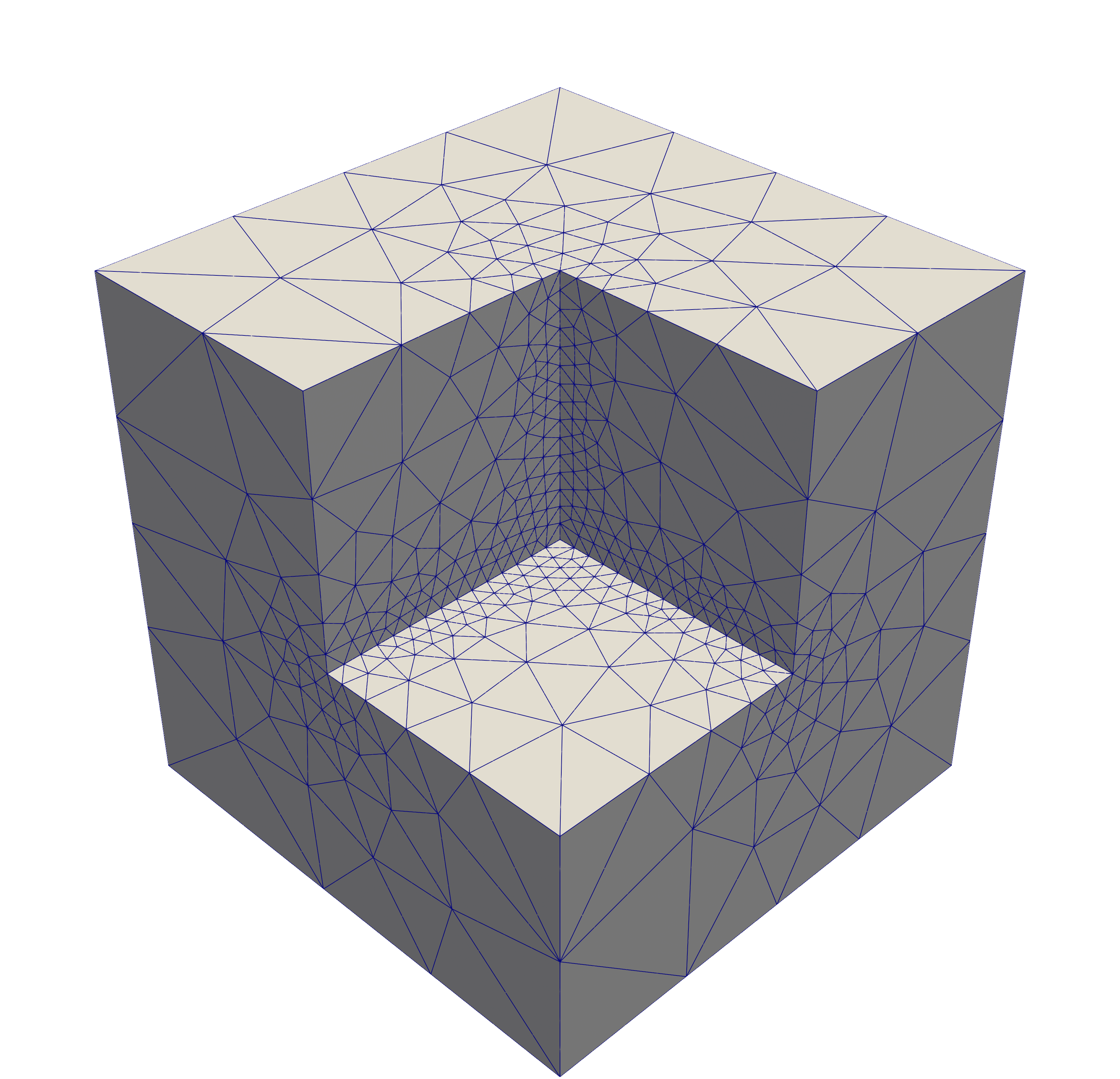
We first discretize each of the Riesz maps 2.6 on an initial Freudenthal mesh of $\Omega=(0,1)^{3}$ with three elements along each edge (see Figure 5(a) for the case of one element per edge) with pure Neumann boundary conditions ( $\Gamma_{N}=\partial\Omega$ ). For each Riesz map, we fix $\beta=1$ , vary $\alpha\in\{10^{3},1,10^{-3}\}$ and $p\in 3:7$ , and perform two levels of mesh refinement following [11]. Note that the meshes resulting from refinement have a smaller shape regularity constant compared to the original Freudenthal mesh, but the shape regularity constant remains bounded away from zero as more refinements are performed. We take the right hand side of the resulting linear system to be a random vector and solve with the preconditioned conjugate gradient (PCG) method with a relative tolerance of $10^{-8}$ .

7.1.1. $H(\operatorname{grad})$ solvers

We consider the subspace decomposition $\mathrm{PAFW}_{0}({X^{0}})$ 6.8 and the corresponding interior-interface splitting $\mathrm{PAFW}_{0}({X^{0}_{\Gamma}})+\mathrm{J}({X^{0}_{\mathcal{I}}})$ 6.9. Here, and in the following examples, we use a symmetric hybrid Schwarz method preconditioner. In particular, the solvers from each group of spaces separated by a “ $+$ ” in the decompositions

(7.1)

\displaystyle X^{k}=W^{k}+\sum_{V\in\Delta_{0}(\mathcal{T}_{h})}\left.X^{k}\right|_{\star V}\quad\text{and}\quad X^{k}=W^{k}+\sum_{V\in\Delta_{0}(\mathcal{T}_{h})}\left.X^{k}_{\Gamma}\right|_{\star V}+\sum_{\ell=1}^{N^{k}_{\mathcal{I}}}\operatorname{span}\left\{\phi_{\ell}^{k}\right\}

are weighted using estimated extremal eigenvalues and combined multiplicatively from right to left to right for symmetry. We equip $W^{0}$ with a geometric multigrid V-cycle with vertex patch relaxation (equivalently point-Jacobi) and a direct Cholesky solve on the coarsest mesh, while the remaining subspaces are equipped with exact solvers.

To more precisely describe the multiplicative splitting and the computation of the weights, we rewrite the hybrid methods in 7.1 as a symmetric multiplicative Schwarz method with inexact solvers:

(7.2)

\displaystyle X^{k}=\sum_{m=1}^{M}X^{k}_{m},

where each space $X^{k}_{m}$ is equipped with a weight $\rho_{m}>0$ and the inexact solver $\rho_{m}\tilde{a}_{m}(\cdot,\cdot)$ , and the multiplicative sweep is done $X^{k}_{1},\ldots,X^{k}_{m},\ldots X^{k}_{1}$ . For example, the second decomposition in 7.1 satisfies

\displaystyle X^{0}_{1}=X^{0}_{\mathcal{I}},\quad X^{0}_{2}=X^{0}_{\Gamma},\quad\text{and}\quad X^{0}_{3}=W^{0},

where $\tilde{a}_{1}(\cdot,\cdot)$ is a point-Jacobi solver, $\tilde{a}_{2}(\cdot,\cdot)$ is the additive Schwarz method with decomposition $\sum_{V\in\Delta_{0}(\mathcal{T}_{h})}\left.X^{0}_{\Gamma}\right|_{\star V}$ and exact solvers (additive patch solver on 0-stars), and $\tilde{a}_{3}(\cdot,\cdot)$ is a geometric multigrid V-cycle as above. The first decomposition in 7.1 can be described similarly. The weight $\rho_{m}$ is taken to be

(7.3)

\rho_{m}=\frac{\tilde{\lambda}_{\min}+3\tilde{\lambda}_{\max}}{4}

where $\tilde{\lambda}_{\min}$ and $\tilde{\lambda}_{\max}$ are estimates of the extreme generalized eigenvalues of

\displaystyle u\in X^{0}_{m},\lambda\in\mathbb{R}:\qquad a(u,v)=\lambda\tilde{a}_{m}(u,v)\qquad\forall v\in X^{0}_{m}

computed from 10 conjugate gradient iterations with a randomized right hand side [34]. With this language, the $\mathrm{PAFW}_{0}({X^{0}_{\Gamma}})+\mathrm{J}({X^{0}_{\mathcal{I}}})$ solver is summarized in Figure 6.

Figure 6. Solver diagram for

\mathrm{PAFW}_{l}({X^{k}_{\Gamma}})+\mathrm{J}({X^{k}_{\mathcal{I}}})

used for

H(\operatorname{grad})

and

H(\operatorname{curl})

(

l=0

) and

H(\operatorname{div})

(

l=1

The iteration counts for the two decompositions in 7.1 with $p\in 5:7$ are displayed in section 7.1.1. Here, and in the tables that follow, each column corresponds to a different value of $\alpha$ , and the number of iterations for the solver with interior-interface splitting are displayed on the left followed by the iteration counts for the corresponding solver without the interior-interface splitting in brackets. We observe that across all values of $\alpha$ and $p$ , the computationally cheaper $\mathrm{PAFW}_{0}({X^{0}_{\Gamma}})+\mathrm{J}({X^{0}_{\mathcal{I}}})$ solver performs within 3 iterations of the full $\mathrm{PAFW}_{0}({X^{0}_{\Gamma}})$ solver, and all of these iteration counts are robust with respect to the $\alpha$ , $p$ , and $h$ .

Table 3. PCG iteration counts for the

H(\operatorname{grad})

Riesz map, where

Y^{0}=X^{0}_{\Gamma}\ (Y^{0}=X^{0})

\csvreader

[ head to column names, head to column names prefix=MY, tabular=rcccc, table head= $\mathrm{PAFW}_{0}({Y^{0}})$
$l$ $p$ $\alpha=10^{3}$ $\alpha=1$ $\alpha=10^{-3}$
, late after line=
, filter ifthen=\equal\MYdegree5 \equal\MYdegree6 \equal\MYdegree7, table foot=]results/CG.3d.demkowicz.afw.combined.csv \MYlevel \MYdegree \MYFAiterations (\MYAiterations) \MYFBiterations (\MYBiterations) \MYFCiterations (\MYCiterations)

7.1.2. $H(\operatorname{curl})$ solvers

We first consider the subspace decompositions based on vertex patches $\mathrm{PAFW}_{0}({X^{1}})$ and $\mathrm{PAFW}_{0}({X^{1}_{\Gamma}})+\mathrm{J}({X^{1}_{\mathcal{I}}})$ using the same symmetric hybrid Schwarz solver described above and in Figure 6. Note that the vertex patch relaxation of the geometric multigrid V-cycle preconditioner on $W^{1}$ is no longer equivalent to a point-Jacobi relaxation. The iteration counts for these two solvers with $p\in\{3,5,7\}$ are displayed in the leftmost section of section 7.1.2. For $\alpha\geq 1$ , $\mathrm{PAFW}_{0}({X^{1}})$ and $\mathrm{PAFW}_{0}({X^{1}_{\Gamma}})+\mathrm{J}({X^{1}_{\mathcal{I}}})$ are within 7 iterations of one another, while for $\alpha=10^{-3}$ , $\mathrm{PAFW}_{0}({X^{1}_{\Gamma}})+\mathrm{J}({X^{1}_{\mathcal{I}}})$ requires about double the number of iterations as $\mathrm{PAFW}_{0}({X^{1}})$ . The robustness of the interior-interface splitting for $\alpha\geq 1$ and its degradation for $\alpha=10^{-3}$ is consistent with the stability of the decomposition in Theorem 6.1.

We now consider two Hiptmair–Toselli variants $\mathrm{HT}({X^{0}},{X^{1}})$ and $\mathrm{HT}({X^{0}},{X^{1,\mathrm{I}}})$ along with their interior-interface splitting counterparts $\mathrm{HT}({X^{0}_{\Gamma}},{X^{1}_{\Gamma}})+\mathrm{J}({X^{1}_{\mathcal{I}}})$ and $\mathrm{HT}({X^{0}_{\Gamma}},{X^{1,\mathrm{I}}_{\Gamma}})+\mathrm{J}({X^{1}_{\mathcal{I}}})$ . We use an analogous hybrid Schwarz method preconditioner as for $\mathrm{PAFW}_{0}({X^{1}})$ . For example, the $\mathrm{HT}({X^{0}_{\Gamma}},{X^{1,\mathrm{I}}_{\Gamma}})+\mathrm{J}({X^{1}_{\mathcal{I}}})$ solver can be expressed as a symmetric multiplicative Schwarz method as in 7.2 with weighted inexact solvers by choosing

\displaystyle X_{1}^{1}=X^{1}_{\mathcal{I}},\quad X^{1}_{2}=X^{1}_{\Gamma},\quad\text{and}\quad X^{1}_{3}=W^{1}.

As above, $\tilde{a}_{1}(\cdot,\cdot)$ is point-Jacobi, while $\tilde{a}_{2}(\cdot,\cdot)$ is the additive Schwarz method associated to the (Hiptmair–Toselli) decomposition

(7.4)

\displaystyle\sum_{V\in\Delta_{0}(\mathcal{T}_{h})}\left.\operatorname{grad}X^{0}_{\Gamma}\right|_{\star V}+\sum_{E\in\Delta_{1}(\mathcal{T}_{h})}\left.X^{1,\mathrm{I}}_{\Gamma}\right|_{\star E}

with exact solvers. The inexact solver $\tilde{a}_{3}(\cdot,\cdot)$ is a geometric multigrid V-cycle preconditioner with Hiptmair–Jacobi smoothing meaning that the smoother is the additive Schwarz method associated to the decomposition 7.4 at lowest order ( $X^{0}_{\Gamma}=W^{0}$ and $X^{1,\mathrm{I}}_{\Gamma}=W^{1}$ ) with exact solvers. The solver is summarized in Figure 7. The other three hybrid Hiptmair–Toselli solvers are defined analogously.

Figure 7. Solver diagram for

\mathrm{HT}({Y_{\Gamma}^{k-1}},{Z_{\Gamma}^{k,\mathrm{I}}})+\mathrm{J}({X^{k}_{\mathcal{I}}})

used for

H(\operatorname{curl})

and

H(\operatorname{div})

The iteration counts for the four Hiptmair–Toselli decompositions are displayed in the two rightmost sections of section 7.1.2. For each fixed value of $\alpha$ , the $\mathrm{HT}({X^{0}},{X^{1}})$ and $\mathrm{HT}({X^{0}_{\Gamma}},{X^{1}_{\Gamma}})+\mathrm{J}({X^{1}_{\mathcal{I}}})$ solvers give nearly identical iteration counts which are robust in $h$ and $p$ . Moreover, the iteration counts are robust across values of $\alpha$ . For $\alpha\geq 1$ , the $\mathrm{HT}({X^{0}},{X^{1,\mathrm{I}}})$ and $\mathrm{HT}({X^{0}_{\Gamma}},{X^{1,\mathrm{I}}_{\Gamma}})+\mathrm{J}({X^{1}_{\mathcal{I}}})$ solvers also give nearly identical iteration counts that are a few iterations less than the $\mathrm{HT}({X^{0}},{X^{1}})$ and $\mathrm{HT}({X^{0}_{\Gamma}},{X^{1}_{\Gamma}})+\mathrm{J}({X^{1}_{\mathcal{I}}})$ solvers. For $\alpha=10^{-3}$ , $\mathrm{HT}({X^{0}_{\Gamma}},{X^{1,\mathrm{I}}_{\Gamma}})+\mathrm{J}({X^{1}_{\mathcal{I}}})$ slightly outperforms $\mathrm{HT}({X^{0}},{X^{1,\mathrm{I}}})$ , but both require substantially more iterations than for $\alpha\geq 1$ and the number of iterations decreases as the mesh is refined. Overall, for $\alpha\geq 1$ , the finest splitting $\mathrm{HT}({X^{0}_{\Gamma}},{X^{1,\mathrm{I}}_{\Gamma}})+\mathrm{J}({X^{1}_{\mathcal{I}}})$ is within 6 iterations of $\mathrm{PAFW}_{0}({X^{1}})$ , which is the most computationally expensive solver and requires the smallest iteration counts, while the slightly coarser splitting $\mathrm{HT}({X^{0}_{\Gamma}},{X^{1}_{\Gamma}})+\mathrm{J}({X^{1}_{\mathcal{I}}})$ requires about 3 times the number of iterations as $\mathrm{PAFW}_{0}({X^{1}})$ for $\alpha=10^{-3}$ .

Table 4. PCG iteration counts for the

H(\operatorname{curl})

Riesz map, where

Y^{k}=X^{k}_{\Gamma}\ (Y^{k}=X^{k})

\csvreader

[ head to column names, head to column names prefix=MY, tabular=rlccc—, table head= $\mathrm{PAFW}_{0}({Y^{1}})$
$l$ $p$ $\alpha=10^{3}$ $\alpha=1$ $\alpha=10^{-3}$
, late after line=
, filter ifthen=\equal\MYdegree3 \equal\MYdegree5 \equal\MYdegree7, table foot=]results/N1curl.3d.demkowicz.afw.combined.csv \MYlevel \MYdegree \MYFAiterations (\MYAiterations) \MYFBiterations (\MYBiterations) \MYFCiterations (\MYCiterations) \csvreader[ head to column names, head to column names prefix=MY, tabular=—ccc, table head= $\mathrm{HT}({Y^{0}},{Y^{1}})$
$\alpha=10^{3}$ $\alpha=1$ $\alpha=10^{-3}$
, late after line=
, filter ifthen=\equal\MYdegree3 \equal\MYdegree5 \equal\MYdegree7, table foot=]results/N1curl.3d.demkowicz.hiptmair.combined.csv \MYFAiterations (\MYAiterations) \MYFBiterations (\MYBiterations) \MYFCiterations (\MYCiterations)

\csvreader

[ head to column names, head to column names prefix=MY, tabular=rlccc, table head= $\mathrm{HT}({Y^{0}},{Y^{1,\mathrm{I}}})$
$l$ $p$ $\alpha=10^{3}$ $\alpha=1$ $\alpha=10^{-3}$
, late after line=
, filter ifthen=\equal\MYdegree3 \equal\MYdegree5 \equal\MYdegree7, table foot=]results/N1curl.3d.demkowicz.hiptmair-red.combined.csv \MYlevel \MYdegree \MYFAiterations (\MYAiterations) \MYFBiterations (\MYBiterations) \MYFCiterations (\MYCiterations)

7.1.3. $H(\operatorname{div})$ solvers

We again first consider the vertex patch subspace decompositions $\mathrm{PAFW}_{0}({X^{3}})$ and $\mathrm{PAFW}_{0}({X_{\Gamma}^{3}})+\mathrm{J}({X_{\mathcal{I}}^{3}})$ with the same symmetric hybrid Schwarz solver described in Figure 6. The iteration counts for these two solvers with $p\in\{3,5,7\}$ are displayed in the upper left quadrant of section 7.1.3. After one or two levels of refinement, $\mathrm{PAFW}_{0}({X_{\Gamma}^{3}})+\mathrm{J}({X_{\mathcal{I}}^{3}})$ requires about double the number of iterations as $\mathrm{PAFW}_{0}({X^{3}})$ , but all iteration counts appear to be robust in $\alpha$ , $h$ , and $p$ . For the edge patch subspace decompositions $\mathrm{PAFW}_{1}({X^{3}})$ and $\mathrm{PAFW}_{1}({X_{\Gamma}^{3}})+\mathrm{J}({X_{\mathcal{I}}^{3}})$ , described in Figure 6 and displayed in the upper right of section 7.1.3, the iteration counts for $\alpha\geq 1$ differ by at most 2 and are insensitive to $\alpha$ and $p$ . For $\alpha=10^{-3}$ , the iteration counts decrease as the mesh is refined and on the finest mesh, the iteration counts are also within 2 and appear to be insensitive to $p$ .

The iteration counts for the Hiptmair–Toselli decompositions $\mathrm{HT}({X^{2}},{X^{3}})$ ,
$\mathrm{HT}({X_{\Gamma}^{2}},{X_{\Gamma}^{3}})+\mathrm{J}({X_{\mathcal{I}}^{3}})$ , $\mathrm{HT}({X^{2,\mathrm{I}}},{X^{3,\mathrm{I}}})$ , and $\mathrm{HT}({X_{\Gamma}^{2,\mathrm{I}}},{X_{\Gamma}^{3,\mathrm{I}}})+\mathrm{J}({X_{\mathcal{I}}^{3}})$ , described in Figure 7, are displayed in the bottom half of section 7.1.3. Note that the results are similar to the edge patch decompositions, with the only exception being that the type-I/type-II splitting $\mathrm{HT}({X^{2,\mathrm{I}}},{X^{3,\mathrm{I}}})$ performs worse than $\mathrm{HT}({X^{2}},{X^{3}})$ on coarser meshes. Overall, $\mathrm{PAFW}_{0}({X^{3}})$ and $\mathrm{PAFW}_{0}({X_{\Gamma}^{3}})+\mathrm{J}({X_{\mathcal{I}}^{3}})$ perform the best, but all solvers with the interior-interface split perform nearly identically for $\alpha\geq 1$ and on fine enough meshes for $\alpha=10^{-3}$ .

Table 5. PCG iteration counts for the

H(\operatorname{div})

Riesz map, where

Y^{k}=X^{k}_{\Gamma}\ (Y^{k}=X^{k})

\csvreader

[ head to column names, head to column names prefix=MY, tabular=rlccc—, table head= $\mathrm{PAFW}_{0}({Y^{2}})$
$l$ $p$ $\alpha=10^{3}$ $\alpha=1$ $\alpha=10^{-3}$
, late after line=
, filter ifthen=\equal\MYdegree3 \equal\MYdegree5 \equal\MYdegree7 ]results/N1div.3d.demkowicz.afw0.combined.csv \MYlevel \MYdegree \MYFAiterations (\MYAiterations) \MYFBiterations (\MYBiterations) \MYFCiterations (\MYCiterations) \csvreader[ head to column names, head to column names prefix=MY, tabular=—ccc, table head= $\mathrm{PAFW}_{1}({Y^{2}})$
$\alpha=10^{3}$ $\alpha=1$ $\alpha=10^{-3}$
, late after line=
, filter ifthen=\equal\MYdegree3 \equal\MYdegree5 \equal\MYdegree7 ]results/N1div.3d.demkowicz.afw.combined.csv \MYFAiterations (\MYAiterations) \MYFBiterations (\MYBiterations) \MYFCiterations (\MYCiterations)

\csvreader

[ head to column names, head to column names prefix=MY, tabular=rlccc—, table head= $\mathrm{HT}({Y^{1}},{Y^{2}})$
$l$ $p$ $\alpha=10^{3}$ $\alpha=1$ $\alpha=10^{-3}$
, late after line=
, filter ifthen=\equal\MYdegree3 \equal\MYdegree5 \equal\MYdegree7, table foot=]results/N1div.3d.demkowicz.hiptmair.combined.csv \MYlevel \MYdegree \MYFAiterations (\MYAiterations) \MYFBiterations (\MYBiterations) \MYFCiterations (\MYCiterations) \csvreader[ head to column names, head to column names prefix=MY, tabular=—ccc, table head= $\mathrm{HT}({Y^{1,\mathrm{I}}},{Y^{2,\mathrm{I}}})$
$\alpha=10^{3}$ $\alpha=1$ $\alpha=10^{-3}$
, late after line=
, filter ifthen=\equal\MYdegree3 \equal\MYdegree5 \equal\MYdegree7, table foot=]results/N1div.3d.demkowicz.hiptmair-red.combined.csv \MYFAiterations (\MYAiterations) \MYFBiterations (\MYBiterations) \MYFCiterations (\MYCiterations)

7.1.4. Summary remarks

For all of the Riesz maps considered, each space decomposition with and without the interior-interface splitting have the same behavior as $h\to 0$ , $p\to\infty$ , and $h^{2}\beta/\alpha\to 0$ , which is consistent with Theorem 6.1. The degradation of the splitting as $h^{2}\beta/\alpha\to\infty$ present in Theorem 6.1 is confirmed by a jump in iteration counts for $l=0$ and $\alpha=10^{-3}$ between $\mathrm{PAFW}_{0}({X^{1}})$ and $\mathrm{PAFW}_{0}({X^{1}_{\Gamma}})+\mathrm{J}({X^{1}_{\mathcal{I}}})$ , between $\mathrm{PAFW}_{0}({X^{2}})$ and $\mathrm{PAFW}_{0}({X^{2}_{\Gamma}})+\mathrm{J}({X^{2}_{\mathcal{I}}})$ , between $\mathrm{PAFW}_{1}({X^{2}})$ and $\mathrm{PAFW}_{1}({X^{2}_{\Gamma}})+\mathrm{J}({X^{2}_{\mathcal{I}}})$ , and between $\mathrm{HT}({X^{1}},{X^{2}})$ and $\mathrm{HT}({X^{1}_{\Gamma}},{X^{2}_{\Gamma}})+\mathrm{J}({X^{2}_{\mathcal{I}}})$ . That the remaining solvers appear to be unaffected by $h^{2}\beta/\alpha$ warrants further theoretical investigation. Also note that the effect of changing shape regularity is observed as there is a slight increase in the iteration counts after one level of mesh refinement. Moreover, Lemma 6.3 seems to partially capture the lack of $p$ -robustness of the type-I/type-II splitting in as observed in $\mathrm{HT}({X^{0}},{X^{1,\mathrm{I}}})$ and $\mathrm{HT}({X_{\Gamma}^{0}},{X_{\Gamma}^{1,\mathrm{I}}})+\mathrm{J}({X_{\mathcal{I}}^{1}})$ when $\alpha=10^{-3}$ . The apparent $p$ -robustness of all the Type-I/Type-II splittings for $\alpha\geq 1$ and for $\mathrm{HT}({X^{1,\mathrm{I}}},{X^{2,\mathrm{I}}})$ for $\alpha=10^{-3}$ is not explained by our current theory.

We again emphasize that the cost of one iteration for the standard solvers, which include all interior degrees of freedom in the patch solves, is significantly more expensive than the solvers with the interior-interface splittings. In the case $h^{2}\beta/\alpha\leq 1$ , all of the iteration counts observed are nearly identical between solvers with and without the interior-interface splitting. Moreover, all solvers with the interior-interface splitting considered for a particular Riesz map gave nearly identical iteration counts. Thus, in the case that $h^{2}\beta/\alpha\leq 1$ , we recommend solvers for each of the Riesz maps as follows. For $H(\operatorname{grad})$ , there is only one choice, $\mathrm{PAFW}_{0}({X^{0}_{\Gamma}})+\mathrm{J}({X^{0}_{\mathcal{I}}})$ . For $H(\operatorname{curl})$ , we take the finest splitting $\mathrm{HT}({X_{\Gamma}^{0}},{X_{\Gamma}^{1,\mathrm{I}}})+\mathrm{J}({X^{1}_{\mathcal{I}}})$ . For $H(\operatorname{div})$ , we take $\mathrm{PAFW}_{1}({X^{2}_{\Gamma}})+\mathrm{J}({X^{2}_{\mathcal{I}}})$ because this decomposition involves patch problems that are only marginally more expensive than the patch problems in the finest splitting $\mathrm{HT}({X^{1,\mathrm{I}}},{X^{2,\mathrm{I}}})+\mathrm{J}({X^{2}_{\mathcal{I}}})$ , as discussed in section 6.3, but avoids the need for an auxiliary space. We will use these decompositions in the next section to precondition the Hodge–Laplace problem.

7.2. Hodge–Laplacians

The Riesz maps are very useful in the construction of block preconditioner for coupled systems of partial differential equations [38]. Here, we employ block diagonal preconditioners based on our developed space decomposition methods for the Riesz maps to solve Hodge–Laplacians [6] on the Fichera corner $\Omega=(0,1)^{3}\setminus(0.5,1)^{3}$ with $\Gamma_{N}=\partial\Omega$ as a prototypical example. For $k\in 1:3$ , the problem is to find $(\sigma,u)\in X^{k-1}\times X^{k}$ such that


(7.5a)	$\displaystyle-(\sigma,\tau)+(u,\operatorname{d}^{k-1}\tau)$	$\displaystyle=0\qquad$	$\displaystyle\forall\tau\in X^{k-1}$
(7.5b)	$\displaystyle(\operatorname{d}^{k-1}\sigma,v)+(\operatorname{d}^{k}u,\operatorname{d}^{k}v)$	$\displaystyle=F(v)\qquad$	$\displaystyle\forall v\in X^{k},$

where we recall that $d^{3}:=0$ . The cases $k\in 1:2$ correspond to a mixed formulation of the vector Poisson problem, while the case $k=3$ yields the mixed formulation of the scalar Poisson problem in $H(\operatorname{div})\times L^{2}$ . We consider a single unstructured mesh, pictured in Figure 5(b). The mesh is refined towards the re-entrant vertex and the edges abutting the vertex, and the diameter of the refined tetrahedra are about $1/8$ the diameter of the largest tetrahedra. We prescribe a constant source term $F(v)=(f,v)$ for a constant $f=1$ or $f=(1,1,1)^{\top}$ .

Since problem 7.5 is well-posed in $H(\operatorname{d}^{k-1})\times H(\operatorname{d}^{k})$ [6], we consider the following block diagonal (weighted) Riesz map preconditioner:

(7.6)

(\sigma,\tau)+(\operatorname{d}^{k-1}\sigma,\gamma\operatorname{d}^{k-1}\tau)+(u,\gamma^{-1}v)+(\operatorname{d}^{k}u,\operatorname{d}^{k}v).

The case $\gamma=1$ corresponds to standard operator preconditioning [38], while $k=3$ and $\gamma\gg 1$ corresponds to augmented Lagrangian preconditioning [23, 27]. For $k\in 1:2$ and $\gamma\neq 1$ , the weighted Riesz map preconditioner 7.6 appears to be novel. We show in Theorem E.1 that if one uses 7.6 to precondition 7.5, then all of the eigenvalues of the preconditioned system converge to $\pm 1$ as $\gamma\to\infty$ .

Of course, the preconditioner 7.6 is too expensive to use directly, so we replace each of the weighted Reisz maps with the hybrid Schwarz method preconditioners we used above. Since we only encounter the case $\beta/\alpha\leq 1$ , we restrict the discussion to the subspace decompositions we recommend in section 7.1.4 and the corresponding decompositions that do not split the interior-interface degrees of freedom:

•

$\mathrm{CG}_{p}$ : $\mathrm{PAFW}_{0}({X^{0}_{\Gamma}})+\mathrm{J}({X^{0}_{\mathcal{I}}})$ (and $\mathrm{PAFW}_{0}({X^{0}})$ ),
•

$\mathrm{Ned}^{1}_{p}$ : $\mathrm{HT}({X_{\Gamma}^{0}},{X_{\Gamma}^{1,\mathrm{I}}})+\mathrm{J}({X^{1}_{\mathcal{I}}})$ (and $\mathrm{HT}({X^{0}},{X^{1,\mathrm{I}}})$ ),
•

$\mathrm{RT}_{p}$ : $\mathrm{PAFW}_{1}({X^{2}_{\Gamma}})+\mathrm{J}({X^{2}_{\mathcal{I}}})$ (and $\mathrm{PAFW}_{1}({X^{2}})$ ),
•

$\mathrm{DG}_{p-1}$ : $\mathrm{J}({X^{3}})$ (and $\mathrm{J}({X^{3}})$ ), an exact solver as the basis is orthogonal.

Table 6. Preconditioned MINRES iteration counts to solve the Hodge Laplacians.

\csvreader

[ head to column names, head to column names prefix=MY, tabular=r@ c@ c@ c@ c—, table head= $\mathrm{CG}_{p}\times\mathrm{Ned}^{1}_{p}$
$p$ $\gamma=1$ $\gamma=10^{3}$
, table foot=]results/hodge.N1curl.3d.demkowicz.combined.csv \MYdegree \MYFAiterations (\MYAiterations) \MYFBiterations (\MYBiterations) \csvreader[ head to column names, head to column names prefix=MY, tabular=—c@ c@ c—, table head= $\mathrm{Ned}^{1}_{p}\times\mathrm{RT}_{p}$
$\gamma=1$ $\gamma=10^{3}$
, table foot=]results/hodge.N1div.3d.demkowicz.combined.csv \MYFAiterations (\MYAiterations) \MYFBiterations (\MYBiterations) \csvreader[ head to column names, head to column names prefix=MY, tabular=—c@ c@ c, table head= $\mathrm{RT}_{p}\times\mathrm{DG}_{p-1}^{\phantom{1}}$
$\gamma=1$ $\gamma=10^{3}$
, filter ifthen=／\equal\MYdegree7, table foot=]results/hodge.DG.3d.demkowicz.combined.csv \MYFAiterations (\MYAiterations) \MYFBiterations (\MYBiterations)

The preconditioned MINRES iteration counts for $p\in 1:6$ and $\gamma\in\{1,10^{3}\}$ with a relative tolerance of $10^{-8}$ are displayed in Section 7.2. First note that for $p=1$ , the solver corresponds to using the exact weighted Riesz map preconditioner 7.6 as the multigrid V-cycle preconditioner reduces to an exact solver. Here, we observe that taking $\gamma=10^{3}$ reduces the iteration counts from 5 or 6 to 3. For $p\geq 2$ , we generally see that the solvers are robust in $p$ and that taking $\gamma$ large reduces the iteration counts at no extra expense in the solver. The effect is minimal for the $H(\operatorname{curl})\times H(\operatorname{div})$ Hodge–Laplacian for high-order Schwarz solvers owing to difficulty of solving the individual Riesz maps. For example, one would expect to apply the Schwarz solvers 3-4 times the iteration counts for a single Riesz map solve if instead, one used the Schwarz solvers as an inner iteration to solve each block of the 7.6. For the $H(\operatorname{curl})\times H(\operatorname{div})$ Hodge–Laplacian, this amounts to about 70-100 iterations, which is in line with our observed iteration counts. We also note that the interior-interface splitting again gives comparable iteration counts within 4 for the $H(\operatorname{curl})\times H(\operatorname{div})$ and $H(\operatorname{div})\times L^{2}$ Hodge–Laplacians and within 16 for the $H(\operatorname{grad})\times H(\operatorname{curl})$ Hodge–Laplacian.

Appendix A Bubble complexes and trace decomposition

Lemma A.1.

The complex 3.6 is exact for all $S\in\Delta_{l}(\hat{T})$ with $l\in k+1:d$ .

Proof.

The case that $S=\hat{T}$ follows from the exactness of the usual finite element de Rham complex with homogeneous boundary conditions (see e.g. [35, Corollary 2]).

The only remaining complex to verify is the case that $S\in\Delta_{2}(\hat{T})$ . One can readily verify that $\mathring{X}_{p}^{0}(S)=\mathrm{P}_{p}(S)\cap H^{1}_{0}(S)$ and

(A.1)

\displaystyle\mathring{X}_{p}^{1}(S)=\begin{cases}(\mathrm{P}_{p-1}(S)^{2}+\mathrm{P}_{p-1}(S)(\Pi_{S}\mathbf{x})^{\perp})\cap H_{0}(\operatorname{curl}{};S)&\text{if }X^{1}_{p}(\hat{T})=\mathrm{Ned}^{1}_{p}(\hat{T}),\\ \mathrm{P}_{p}(S)^{2}\cap H_{0}(\operatorname{curl}{};S)&\text{if }X^{1}_{p}(\hat{T})=\mathrm{Ned}^{2}_{p}(\hat{T}),\end{cases}

which is the usual 2D Nedéléc space of first or second kind with vanishing tangential trace. The exactness of 3.6 again follows from [35, Corollary 2]. ∎

Lemma A.2.

The decomposition 3.9 holds.

Proof.

Let $S\in\Delta_{k}(\hat{T})$ . Direct calculation revels that $\operatorname{tr}^{k}_{S}W^{k}(\hat{T})=\mathbb{R}$ . Define $\tau\in\{0,1\}$ as follows: Let $\tau=1$ if $k=0$ or $X^{k}(\hat{T})$ is of the first kind and $\tau=0$ otherwise. Then, direct calculation shows that

\displaystyle\operatorname{tr}^{k}_{S}X^{k}(\hat{T})=\mathrm{P}_{p-\tau}(S)\qquad\operatorname{\forall}S\in\Delta_{k}(\hat{T}).

If $k=1$ , then $\mathring{X}^{0}(S)=\mathcal{P}_{p+1-\tau}(S)\cap H^{1}_{0}(S)$ , while if $k=2$ , then $\mathring{X}^{1}(S)$ is given by A.1 with $p$ replaced by $p+1-\tau$ . [35, Corollary 2] then implies that the following sequence is exact

and the result now follows. ∎

Appendix B Energy stable splittings

By construction, the space $X^{k}$ admits direct sum decompositions based on splitting the interior and interface basis functions and based on splitting the type- $\mathrm{I}$ and type- $\mathrm{II}$ basis functions:

(B.1)

\displaystyle X^{k}=X^{k}_{\Gamma}\oplus X^{k}_{\mathcal{I}}\quad\text{and}\quad X^{k}=X^{k,\mathrm{I}}\oplus X^{k,\mathrm{II}}.

We now examine the energy stability of these two decompositions. Given a domain $\omega$ , let

\displaystyle(u,v)_{H(\operatorname{d}^{k};\omega)}:=(u,v)_{\omega}+(\operatorname{d}^{k}u,\operatorname{d}^{k}v)_{\omega}\quad\text{and}\quad\|u\|_{H(\operatorname{d}^{k};\omega)}^{2}:=(u,u)_{H(\operatorname{d}^{k};\omega)}.

B.1. $H(\operatorname{d}^{k})$ -stability on the reference cell

We begin by analyzing the stability of the decompositions on the reference cell:

(B.2)

\displaystyle X^{k}(\hat{T})=X^{k}_{\Gamma}(\hat{T})\oplus X^{k}_{\mathcal{I}}(\hat{T})\quad\text{and}\quad X^{k}(\hat{T})=X^{k,\mathrm{I}}(\hat{T})\oplus X^{k,\mathrm{II}}(\hat{T}),

where $X^{k}_{\Gamma}(\hat{T})$ , etc. denotes the space analogous to 5.1, 5.2 and 6.1 on the reference cell. In particular, given $u\in X^{k}(\hat{T})$ , there exist unique $u_{\Gamma}\in X^{k}_{\Gamma}(\hat{T})$ , $u_{\mathcal{I}}\in X^{k}_{\mathcal{I}}(\hat{T})$ , $u_{\mathrm{I}}\in X^{k,\mathrm{I}}(\hat{T})$ , and $u_{\mathrm{II}}\in X^{k,\mathrm{II}}(\hat{T})$ such that

(B.3)

\displaystyle u=u_{\Gamma}+u_{\mathcal{I}}\quad\text{and}\quad u=u_{\mathrm{I}}+u_{\mathrm{II}},

and the mappings $u\mapsto(u_{\Gamma},u_{\mathcal{I}})$ and $u\mapsto(u_{\mathrm{I}},u_{\mathrm{II}})$ are linear. The first result shows that the interior-interface decomposition is uniformly stable with respect to the polynomial degree.

Theorem B.1.

There exists a constant $C$ depending only on the dimension $d$ such that for all $u\in X^{k}(\hat{T})$ , there holds

(B.4)

\displaystyle\frac{1}{2}\|u\|_{\hat{T}}^{2}\leq\|u_{\Gamma}\|_{\hat{T}}^{2}+\|u_{\mathcal{I}}\|_{\hat{T}}^{2}\leq C\|u\|_{H(\operatorname{d}^{k};\hat{T})}^{2}

and

(B.5)

\displaystyle\|\operatorname{d}^{k}u\|_{\hat{T}}^{2}=\|\operatorname{d}^{k}u_{\Gamma}\|_{\hat{T}}^{2}+\|\operatorname{d}^{k}u_{\mathcal{I}}\|_{\hat{T}}^{2}.

Proof.

We prove the case $d=3$ ; the case $d=2$ follows from analogous arguments.

Step 1: $\operatorname{d}^{k}$ stability. The degrees of freedom 3.14b and 3.14c show that $u_{\mathcal{I}}$ satisfies


(B.6a)	$\displaystyle(u_{\mathcal{I}},\operatorname{d}^{k-1}y)_{\hat{T}}$	$\displaystyle=(u,\operatorname{d}^{k-1}y)_{\hat{T}}\qquad$	$\displaystyle\operatorname{\forall}y\in\mathring{X}^{k-1}(\hat{T}),$
(B.6b)	$\displaystyle(\operatorname{d}^{k}u_{\mathcal{I}},\operatorname{d}^{k}v)_{\hat{T}}$	$\displaystyle=(\operatorname{d}^{k}u,\operatorname{d}^{k}v)_{\hat{T}}\qquad$	$\displaystyle\operatorname{\forall}v\in\mathring{X}^{k}(\hat{T}),$

and in particular $\operatorname{d}^{k}u_{\mathcal{I}}$ is the $L^{2}(\hat{T})$ -projection of $\operatorname{d}^{k}u$ onto $\operatorname{d}^{k}\mathring{X}^{k}(\hat{T})$ . Equation B.5 immediately follows.

Step 2: $L^{2}$ -stability. Suppose first that $k=0$ . Then, Poincaré’s inequality gives $\|u_{\mathcal{I}}\|_{\hat{T}}\leq C\|u\|_{H(\operatorname{d}^{k};\hat{T})}$ . Now suppose that $k\in\{1,2\}$ . Then, conditions B.6 ensure that there exists $q\in\operatorname{d}^{k}\mathring{X}^{k}(\hat{T})$ such that


(B.7a)	$\displaystyle(u_{\mathcal{I}},v)_{\hat{T}}+(\operatorname{d}^{k}v,q)_{\hat{T}}$	$\displaystyle=(u,v)_{\hat{T}}\qquad$	$\displaystyle\operatorname{\forall}v\in\mathring{X}^{k}(\hat{T}),$
(B.7b)	$\displaystyle(\operatorname{d}^{k}u_{\mathcal{I}},r)_{\hat{T}}$	$\displaystyle=(\operatorname{d}^{k}u,r)_{\hat{T}}\qquad$	$\displaystyle\operatorname{\forall}r\in\operatorname{d}^{k}\mathring{X}^{k}(\hat{T}).$

Applying standard estimates for saddle point systems gives

\displaystyle\|u_{\mathcal{I}}\|_{H(\operatorname{d}^{k};\hat{T})}\leq C(\beta^{k})^{-2}\|u\|_{H(\operatorname{d}^{k};\hat{T})},

where $\beta^{k}$ is the inf-sup constant

\displaystyle\beta^{k}:=\inf_{0\neq r\in\operatorname{d}^{k}\mathring{X}^{k}(\hat{T})}\sup_{0\neq v\in\mathring{X}^{k}(\hat{T})}\frac{(\operatorname{d}^{k}v,r)_{\hat{T}}}{\|v\|_{H(\operatorname{d}^{k},\hat{T})}\|r\|}.

We now show that $\beta^{k}\geq\beta_{0}>0$ for some $\beta_{0}$ independent of $p$ . Let $r\in\operatorname{d}^{k}\mathring{X}^{k}(\hat{T})$ be given. Thanks to [20, Theorem 5.1], there exists $v\in\mathring{X}^{k}(\hat{T})$ such that $\operatorname{d}^{k}v=r$ and $\|v\|_{\hat{T}}\leq C\|r\|_{\hat{T}}$ , where $C$ is independent of $p$ and $r$ . Then, $\|v\|_{H(\operatorname{d}^{k},\hat{T})}\leq C\|r\|_{\hat{T}}$ , and so $\beta^{k}\geq C^{-1}>0$ . Consequently, for $k\in 0:2$ , there holds $\|u_{\mathcal{I}}\|_{H(\operatorname{d}^{k},\hat{T})}\leq C\|u\|_{H(\operatorname{d}^{k},\hat{T})}$ . Inequality B.4 then follows. ∎

We now turn to the type- $\mathrm{I}$ /type- $\mathrm{II}$ decomposition. Let $\{u_{j}^{k},\omega_{j,p}^{k,\mathrm{I}/\mathrm{II}}:j\in 1:\dim X^{k}(\hat{T})\}\subset X^{k}(\hat{T})\times\mathbb{R}$ denote the eigenfunctions and eigenvalues (in increasing order) of the following eigenvalue problem:


(B.8a)	$\displaystyle(u_{i}^{k},u_{j}^{k})_{\hat{T}}$	$\displaystyle=\omega_{i,p}^{k,\mathrm{I}/\mathrm{II}}\delta_{ij}\qquad$	$\displaystyle\operatorname{\forall}i,j\in 1:\dim X^{k}(\hat{T}),$
(B.8b)	$\displaystyle(u_{i,\mathrm{I}}^{k},u^{k}_{j,\mathrm{I}})_{\hat{T}}+(u_{i,\mathrm{II}}^{k},u_{j,\mathrm{II}}^{k})_{\hat{T}}$	$\displaystyle=\delta_{ij}\qquad$	$\displaystyle\operatorname{\forall}i,j\in 1:\dim X^{k}(\hat{T}).$

Then, the following result shows that the $L^{2}(\hat{K})$ stability of the type- $\mathrm{I}$ /type- $\mathrm{II}$ decomposition is determined by the minimal eigenvalue $\omega_{1,p}^{k,\mathrm{I}/\mathrm{II}}$ .

Lemma B.2.

For all $u\in X^{k}(\hat{T})$ , $\operatorname{d}^{k}u=\operatorname{d}^{k}u_{\mathrm{I}}$ and there holds

(B.9)

\displaystyle\frac{1}{2}\|u\|_{\hat{T}}^{2}\leq\|u_{\mathrm{I}}\|_{\hat{T}}^{2}+\|u_{\mathrm{II}}\|_{\hat{T}}^{2}\leq\frac{1}{\omega_{1,p}^{k,\mathrm{I}/\mathrm{II}}}\|u\|_{\hat{T}}^{2}.

Proof.

Since $X^{k,\mathrm{II}}(\hat{T})\subset\ker(\operatorname{d}^{k};X^{k}(\hat{T}))$ thanks to Lemma 4.3, $\operatorname{d}^{k}u=\operatorname{d}^{k}u_{\mathrm{I}}$ . Moreover, let $c_{j}\in\mathbb{R}$ be such that $u=\sum_{j=1}^{\dim X^{k}(\hat{T})}c_{j}u_{j}^{k}$ . Then, applying B.8 gives

\displaystyle\|u_{\mathrm{I}}\|_{\hat{T}}^{2}+\|u_{\mathrm{II}}\|_{\hat{T}}^{2}=\sum_{j=1}^{\dim X^{k}(\hat{T})}c_{j}^{2}\leq\frac{1}{\omega_{1,p}^{k,\mathrm{I}/\mathrm{II}}}\sum_{j=1}^{\dim X^{k}(\hat{T})}c_{j}^{2}\omega_{j,p}^{k,\mathrm{I}/\mathrm{II}}=\|u\|_{\hat{T}}^{2}.

∎

B.2. Energy stability on physical cell

Given an element in $T\in\mathcal{T}_{h}$ and $u\in X^{k}$ , define

\displaystyle a_{T}^{k}(u,v):=(u,\beta v)_{T}+(\operatorname{d}^{k}u,\alpha\operatorname{d}^{k}v)_{T}\ \ \text{and}\ \ \|u\|_{a,T}^{2}:=a_{T}^{k}(u,u)\qquad\operatorname{\forall}u,v\in X^{k}(T).

We again use the notation $u_{\Gamma}$ , $u_{\mathcal{I}}$ , $u_{\mathrm{I}}$ , and $u_{\mathrm{II}}$ to denote the decomposition of $u\in X^{k}$ into its components in the decompositions B.1. The next result shows that these decompositions are energy stable.

Corollary B.3.

There exist constants $C_{1},C_{2}>0$ depending only on shape regularity, $d$ , and $k$ such that for all $u\in X^{k}_{p}(\mathcal{T}_{h})$ and $T\in\mathcal{T}_{h}$ , there holds

(B.10)		$\displaystyle\frac{1}{2}\\|u\\|_{a,T}^{2}$	$\displaystyle\leq\\|u_{\Gamma}\\|_{a,T}^{2}+\\|u_{\mathcal{I}}\\|_{a,T}^{2}$	$\displaystyle\leq C_{1}\max\left\{1,\frac{\beta}{\alpha}h_{T}^{2}\right\}\\|u\\|_{a,T}^{2},$
(B.11)		$\displaystyle\frac{1}{2}\\|u\\|_{a,T}^{2}$	$\displaystyle\leq\\|u_{\mathrm{I}}\\|_{a,T}^{2}+\\|u_{\mathrm{II}}\\|_{a,T}^{2}$	$\displaystyle\leq\frac{C_{2}}{\omega_{1,p}^{k,\mathrm{I}/\mathrm{II}}}\\|u\\|_{a,T}^{2},$

where $\omega_{1,p}^{k,\mathrm{I}/\mathrm{II}}$ is defined in B.8.

Proof.

Let $T\in\mathcal{T}_{h}$ and $\hat{u}:=(\mathcal{F}_{T}^{k})^{-1}u$ so that $\operatorname{d}^{k}u=\mathcal{F}_{T}^{k+1}(\operatorname{d}^{k}\hat{u})$ .

Step 1: $H(\operatorname{d}^{k};T)$ -stability of $u_{\mathcal{I}}$ . Note that $\mathcal{F}^{k}_{T}$ is of the form $\mathcal{F}^{k}_{T}\hat{v}=G_{T}^{k}\hat{v}\circ F_{T}^{-1}$ for some constant or matrix $G^{k}_{T}$ . Thus, there holds

	$\displaystyle\\|u_{\mathcal{I}}\\|_{T}^{2}=\|\det J_{T}\|\cdot\\|G^{k}_{T}\Pi_{\hat{T},\mathcal{I}}^{k}\hat{u}\\|_{\hat{T}}^{2}$	$\displaystyle\leq\|\det J_{T}\|\cdot\|G^{k}_{T}\|^{2}\\|\Pi_{\hat{T},\mathcal{I}}^{k}\hat{u}\\|_{\hat{T}}^{2}$
		$\displaystyle\leq\|\det J_{T}\|\cdot\|G^{k}_{T}\|^{2}\left(\\|\hat{u}\\|_{\hat{T}}^{2}+\\|\operatorname{d}^{k}\hat{u}\\|_{\hat{T}}\\|^{2}\right),$

where $|G^{k}_{T}|$ also denotes the spectral norm on matrices. Now,

\displaystyle\|\hat{u}\|_{\hat{T}}^{2}=|\det J_{T}^{-1}|\cdot\|(G^{k}_{T})^{-1}u\|_{T}^{2}\leq|\det J_{T}|^{-1}|(G^{k}_{T})^{-1}|^{2}\|u\|_{T}^{2}

and

\displaystyle\|\operatorname{d}^{k}\hat{u}\|_{\hat{T}}^{2}=|\det J_{T}^{-1}|\cdot\|(G^{k+1}_{T})^{-1}\operatorname{d}^{k}u\|_{T}^{2}\leq|\det J_{T}|^{-1}|(G^{k+1}_{T})^{-1}|^{2}\|\operatorname{d}^{k}u\|_{T}^{2},

and so

\displaystyle\|u_{\mathcal{I}}\|_{T}^{2}\leq|G^{k}_{T}|^{2}\left(|(G^{k}_{T})^{-1}|^{2}\|u\|_{T}^{2}+|(G^{k+1}_{T})^{-1}|^{2}\|\operatorname{d}^{k}u\|_{T}^{2}\right).

One may then verify that $|G^{k}_{T}|\cdot|(G^{k}_{T})^{-1}|\leq C$ and $|G^{k}_{T}|\cdot|(G^{k+1}_{T})^{-1}|\leq Ch_{T}$ for some $C>0$ depending only on shape regularity, $d$ , and $k$ . Thus,

\displaystyle\|u_{\mathcal{I}}\|_{T}^{2}\leq C\left(\|u\|_{T}^{2}+h_{T}^{2}\|\operatorname{d}^{k}u\|_{T}^{2}\right).

Similar scaling arguments applied to B.5 show that

(B.12)

\displaystyle\|\operatorname{d}^{k}u_{\mathcal{I}}\|_{T}\leq C\|\operatorname{d}^{k}u\|_{T}.

Step 2: B.10. We then obtain

	$\displaystyle(u_{\mathcal{I}},\beta u_{\mathcal{I}})_{T}$	$\displaystyle\leq C\beta\left\{(u,u)_{T}+h_{T}^{2}(\operatorname{d}^{k}u,\operatorname{d}^{k}u)_{T}\right\}$
		$\displaystyle\leq C\left\{(u,\beta u)_{T}+\frac{\beta}{\alpha}h_{T}^{2}(\operatorname{d}^{k}u,\alpha\operatorname{d}^{k}u)_{T}\right\}\leq C\max\left\{1,\frac{\beta}{\alpha}h_{T}^{2}\right\}a^{k}_{T}(u,u),$

and so B.12 gives

\displaystyle a^{k}_{T}(u_{\mathcal{I}},u_{\mathcal{I}})\leq C\max\left\{1,\frac{\beta}{\alpha}h_{T}^{2}\right\}a^{k}_{T}(u,u).

Inequality B.10 now follows from the bound $\|u_{\Gamma}\|_{a,T}^{2}\leq 2\left(\|u\|_{a,T}^{2}+\|u_{\mathcal{I}}\|_{a,T}^{2}\right)$ .

Step 3: B.11. Inequality B.11 follows from Lemma B.2 using analogous arguments from Steps 1 and 2 on noting that $\omega_{1,p}^{k,\mathrm{I}/\mathrm{II}}\leq 2$ by B.9. ∎

We may further decompose the interior component into individual basis functions, and this decomposition is stable for any choice of $\alpha$ and $\beta$ .

Lemma B.4.

Let $N_{K,\mathcal{I}}:=\dim\mathring{X}^{k}(T)$ and let $\{\phi_{T,i}^{k}:i\in 1:N_{K,\mathcal{I}}\}$ denote interior basis functions supported on $T$ . Then, there exists a constant $C>0$ depending only on shape regularity such that if $u_{\mathcal{I}}=\sum_{i=1}^{N_{K,\mathcal{I}}}u_{\mathcal{I},i}\phi_{T,i}^{k}$ , then

(B.13)

\displaystyle C^{-1}\|u_{\mathcal{I}}\|_{a,T}^{2}\leq\sum_{i=1}^{N_{K,\mathcal{I}}}|u_{\mathcal{I},i}|^{2}\|\phi_{T,i}^{k}\|_{a,T}^{2}\leq C\|u_{\mathcal{I}}\|_{a,T}^{2}.

Proof.

Thanks to Lemma 4.5, B.13 holds in the case that $T=\hat{T}$ is the reference cell and $(\alpha,\beta)\in\{(0,1),(1,0)\}$ . A standard scaling argument similar to the one in Step 1 of the proof of Corollary B.3 shows that B.13 holds for all $T\in\mathcal{T}_{h}$ and $(\alpha,\beta)\in\{(0,1),(1,0)\}$ , where $C$ only depend on shape regularity. The case of general $\alpha$ and $\beta$ follows from linearity. ∎

B.3. Proof of Lemma 5.3

The result follows from Theorem 6.1 applied on to a single element with $X_{0}^{k}=X^{k}$ . ∎

Appendix C Proof of Theorem 6.1

Step 1: Stable decomposition 6.6. Let $u\in X^{k}$ and let $\Pi^{k}_{\mathcal{I}}:X^{k}\to X^{k}_{\mathcal{I}}$ be defined by the rule

\displaystyle\Pi^{k}_{\mathcal{I}}v:=v_{\mathcal{I}}\qquad\forall v\in X^{k}.

Note that $\Pi^{k}_{\mathcal{I}}$ is a projection operator. Thanks to 6.5, there exist $u_{m}\in X_{m}$ , $m\in 1:M$ , satisfying

\displaystyle\sum_{m=1}^{M}u_{m}=u\quad\text{and}\quad\sum_{m=1}^{M}\|u_{m}\|_{a}^{2}\leq C_{\mathrm{stable}}(\alpha,\beta)\|u\|_{a}^{2},

where let $\|\cdot\|_{a}$ denotes the energy norm: $\|\cdot\|_{a}^{2}:=a^{k}(\cdot,\cdot)$ . Let $u_{m,\Gamma}:=(I-\Pi_{\mathcal{I}}^{k})u_{m}$ and $u_{\mathcal{I}}:=\Pi_{\mathcal{I}}^{k}u$ . Since $\Pi^{k}_{\mathcal{I}}$ is a projection, there holds

\displaystyle\sum_{i=1}^{M}u_{m,\Gamma}+u_{\mathcal{I}}=(I-\Pi_{\mathcal{I}}^{k})\sum_{i=1}^{M}u_{m}+\Pi_{\mathcal{I}}^{k}u=(I-\Pi_{\mathcal{I}}^{k})u+\Pi_{\mathcal{I}}^{k}u=u,

and applying B.10 element-by-element gives

\displaystyle\sum_{m=1}^{M}\|u_{m,\Gamma}\|_{a}^{2}\leq C\max\left\{1,\frac{\beta}{\alpha}h^{2}\right\}\sum_{m=1}^{M}\|u_{m}\|_{a}^{2}\leq CC_{\mathrm{stable}}(\alpha,\beta)\max\left\{1,\frac{\beta}{\alpha}h^{2}\right\}\|u\|_{a}^{2}.

Consequently, there holds

\displaystyle\|u_{\mathcal{I}}\|_{a}^{2}\leq C\max\left\{1,\frac{\beta}{\alpha}h^{2}\right\}\|u\|_{a}^{2}.

Summing B.13 over the elements then gives

\displaystyle a_{\mathcal{I}}^{k}(u_{\mathcal{I}},u_{\mathcal{I}})+\sum_{m=0}^{M}\|u_{m,\Gamma}\|_{a}^{2}\leq CC_{\mathrm{stable}}(\alpha,\beta)\max\left\{1,\frac{\beta}{\alpha}h^{2}\right\}\|u\|_{a}^{2},

which completes the proof of 6.6.

Step 2: Local Stability. Inequality 6.7 follows immediately from B.13. ∎

Appendix D Further discussion of $\mathrm{HT}({X^{k-1,\mathrm{I}}},{X^{k,\mathrm{I}}})$

We first prove Lemma 6.3 and then discuss the $p$ -dependence of the constant $C_{\mathrm{I}/\mathrm{II}}$ .

D.1. Proof of Lemma 6.3

Let $u\in X^{k}$ and let $u_{0}\in W^{k}$ , $u_{J}\in\left.\operatorname{d}^{k-1}X^{k-1}\right|_{\star J}$ , $J\in\Delta_{k-1}(\mathcal{T}_{h})$ , and $u_{L}\in\left.X^{k}\right|_{\star L}$ , $L\in\Delta_{k}(\mathcal{T}_{h})$ , be such that

	$\displaystyle u_{0}+\sum_{J\in\Delta_{k-1}(\mathcal{T}_{h})}u_{J}+\sum_{L\in\Delta_{k}(\mathcal{T}_{h})}u_{L}$	$\displaystyle=u,$
	$\displaystyle\\|u_{0}\\|_{a}^{2}+\sum_{J\in\Delta_{k-1}(\mathcal{T}_{h})}\\|u_{J}\\|_{a}^{2}+\sum_{L\in\Delta_{k}(\mathcal{T}_{h})}\\|u_{L}\\|_{a}^{2}$	$\displaystyle\leq C_{\mathrm{HT}}\\|u\\|_{a}^{2},$

where $\|\cdot\|_{a}$ again denotes the energy norm. Thanks to 5.7, $\left.\operatorname{d}^{k-1}X^{k-1}\right|_{\star J}=\left.\operatorname{d}^{k-1}X^{k-1,\mathrm{I}}\right|_{\star J}$ , and so $u_{J}\in\left.\operatorname{d}^{k-1}X^{k-1,\mathrm{I}}\right|_{\star J}$ for all $J\in\Delta_{k-1}(\mathcal{T}_{h})$ .

For each $L\in\Delta_{k}(\mathcal{T}_{h})$ , there exist unique $u_{L,\mathrm{I}}\in\left.X^{k,\mathrm{I}}\right|_{\star L}$ and $u_{L,\mathrm{II}}\in\left.X^{k,\mathrm{II}}\right|_{\star L}$ such that $u_{L}=u_{L,\mathrm{I}}+u_{L,\mathrm{II}}$ thanks to 5.3 restricted to $\star L$ . Moreover, summing B.11 over the cells in $\star L$ , we obtain

(D.1)

\displaystyle\|u_{L,\mathrm{I}}\|_{a,\star L}^{2}+\|u_{L,\mathrm{II}}\|_{a,\star L}^{2}

\displaystyle\leq\frac{C}{\omega_{1,p}^{k,\mathrm{I}/\mathrm{II}}}\|u_{L}\|_{a,\star L}^{2}.

Thanks to [35, Corollary 2], the complex

is exact since $\star L$ is contractible, and so $u_{L,\mathrm{II}}\in\operatorname{d}^{k-1}\left.X^{k-1}\right|_{\star L}=\operatorname{d}^{k-1}\left.X^{k-1,\mathrm{I}}\right|_{\star L}$ .

For $J\in\Delta_{k-1}(\mathcal{T}_{h})$ , let $\Delta_{k}(J)$ denote that subsimplices of $J$ of dimension $k$ and define

\displaystyle\tilde{u}_{J}=u_{J}+\frac{1}{|\Delta_{k}(J)|}\sum_{L\in\Delta_{k}(J)}u_{L,\mathrm{II}}.

Then, $\tilde{u}_{J}\in\operatorname{d}^{k-1}\left.X^{k-1,\mathrm{I}}\right|_{\star L}$ and

\displaystyle\|\tilde{u}_{J}\|_{a}^{2}\leq 2\left(\|u_{J}\|_{a}^{2}+\frac{1}{|\Delta_{k}(J)|}\sum_{L\in\Delta_{k}(J)}\|u_{L,\mathrm{II}}\|_{a}^{2}\right).

Consequently, there holds

\displaystyle u_{0}+\sum_{J\in\Delta_{k-1}(\mathcal{T}_{h})}\tilde{u}_{J}+\sum_{L\in\Delta_{k}(\mathcal{T}_{h})}u_{L,\mathrm{I}}=u_{0}+\sum_{J\in\Delta_{k-1}(\mathcal{T}_{h})}u_{J}+\sum_{L\in\Delta_{k}(\mathcal{T}_{h})}u_{L}=u,

and applying D.1 gives

	$\displaystyle\\|u_{0}\\|_{a}^{2}+\sum_{J\in\Delta_{k-1}(\mathcal{T}_{h})}\\|\tilde{u}_{J}\\|_{a}^{2}+\sum_{L\in\Delta_{k}(\mathcal{T}_{h})}\\|u_{L,\mathrm{I}}\\|_{a}^{2}$
	$\displaystyle\qquad\leq 2\left(\\|u_{0}\\|_{a}^{2}+\sum_{J\in\Delta_{k-1}(\mathcal{T}_{h})}\\|\tilde{u}_{J}\\|_{a}^{2}+\sum_{L\in\Delta_{k}(\mathcal{T}_{h})}\left(\\|u_{L,\mathrm{I}}\\|_{a}^{2}+\\|u_{L,\mathrm{II}}\\|_{a}^{2}\right)\right)$
	$\displaystyle\qquad\leq C_{\mathrm{HT}}\frac{C}{\omega_{1,p}^{k,\mathrm{I}/\mathrm{II}}}\\|u\\|_{a}^{2},$

which completes the proof with $C_{\mathrm{I}/\mathrm{II}}=C/\omega_{1,p}^{k,\mathrm{I}/\mathrm{II}}$ . ∎

D.2. The $p$ -dependence of $C_{\mathrm{I}/\mathrm{II}}$

The previous section shows that we may take $C_{\mathrm{I}/\mathrm{II}}=C/\omega_{1,p}^{k,\mathrm{I}/\mathrm{II}}$ in Lemma 6.3. We show the values of $\omega_{1,p}^{k,\mathrm{I}/\mathrm{II}}$ for $\mathrm{Ned}^{1}_{p}$ and $\mathrm{RT}_{p}$ with $p\in 1:10$ in Figure 8. It appears that $\omega_{1,p}^{1,\mathrm{I}/\mathrm{II}}\sim\mathcal{O}(p^{-3})$ , while $\omega_{1,p}^{2,\mathrm{I}/\mathrm{II}}\sim\mathcal{O}(p^{-2})$ . Thus, the type-I/type-II splitting approach may incur an algebraic factor of $p$ in the condition number estimate for the Riesz map problems. However, we only observed such a drastic growth in terms of iteration counts for the solvers $\mathrm{HT}({X^{0}},{X^{1,\mathrm{I}}})$ and $\mathrm{HT}({X_{\Gamma}^{0}},{X_{\Gamma}^{1,\mathrm{I}}})+\mathrm{J}({X^{1}_{\mathcal{I}}})$ when $\alpha=10^{-3}$ and $\beta=1$ , as shown in section 7.1.2.

Figure 8. Type based decoupling constant

\omega^{k,\mathrm{I}/\mathrm{II}}_{1,p}

on an equilateral reference tetrahedron.

Appendix E Augmented Lagrangian preconditioning for Hodge Laplacians

We first recall a few properties of Hilbert complexes from [5]. Let $(\{W^{k}\},\{\operatorname{d}^{k}\})$ be a Hilbert complex with inner-product $\langle\cdot,\cdot\rangle$ inducing the norm $\|\cdot\|$ , and let $(\{V^{k}\},\{\operatorname{d}^{k}\})$ be the associated domain complex:

(E.1)

where the inner-product on $V^{k}$ is $\langle\cdot,\cdot\rangle+\langle\operatorname{d}^{k}\cdot,\operatorname{d}^{k}\cdot\rangle$ . The complex induces the Hodge decomposition

(E.2)

\displaystyle V^{k}=\mathfrak{B}^{k}\oplus\mathfrak{H}^{k}\oplus\mathfrak{Z}^{k,\perp},

where $\mathfrak{B}^{k}$ is the image of $\operatorname{d}^{k-1}$ , $\mathfrak{H}^{k}$ is the space of harmonic forms, and $\mathfrak{Z}^{k,\perp}$ is the orthogonal complement of the kernel of $\operatorname{d}^{k}$ :

	$\displaystyle\mathfrak{B}^{k}$	$\displaystyle:=\operatorname{d}^{k-1}V^{k-1}=\operatorname{d}^{k-1}\mathfrak{Z}^{k-1,\perp},$
	$\displaystyle\mathfrak{H}^{k}$	$\displaystyle:=\{\mathfrak{h}\in V^{k}:\operatorname{d}^{k}\mathfrak{h}=0\text{ and }\langle\mathfrak{h},\operatorname{d}^{k-1}\sigma\rangle=0\ \forall\sigma\in V^{k-1}\},$
	$\displaystyle\mathfrak{Z}^{k,\perp}$	$\displaystyle:=\{v\in V^{k}:\langle v,z\rangle=0\ \forall z\in V^{k}\text{ with }\operatorname{d}^{k}z=0\}.$

Note that the Hodge decomposition is orthogonal with respect to the inner-product on $W^{k}$ and on $V^{k}$ . Moreover, given $v\in V^{k}$ , we write $v=v_{\mathfrak{B}}+v_{\mathfrak{H}}+v_{\perp}$ to denote the Hodge decomposition of $v$ .

The mixed formulation of the Hodge Laplace problem associated to E.1 reads as follows: Find $(\sigma,u,p)\in V^{k-1}\times V^{k}\times\mathfrak{H}^{k}$ such that


(E.3a)	$\displaystyle-\langle\sigma,\tau\rangle+\langle u,\operatorname{d}^{k-1}\tau\rangle$	$\displaystyle=0\qquad$	$\displaystyle\forall\tau\in V^{k-1},$
(E.3b)	$\displaystyle\langle\operatorname{d}^{k-1}\sigma,v\rangle+\langle p,v\rangle+\langle\operatorname{d}^{k}u,\operatorname{d}^{k}v\rangle$	$\displaystyle=\langle f,v\rangle\qquad$	$\displaystyle\forall v\in V^{k},$
(E.3c)	$\displaystyle\langle u,q\rangle$	$\displaystyle=0\qquad$	$\displaystyle\forall q\in\mathfrak{H}^{k}.$

We may combine the bilinear forms in E.3 into one large symmetric bilinear form

\displaystyle A(\sigma,u,p;\tau,v,q):=\langle\operatorname{d}^{k}u,\operatorname{d}^{k}v\rangle+\langle\operatorname{d}^{k-1}\sigma,v\rangle+\langle u,\operatorname{d}^{k-1}\tau\rangle-\langle\sigma,\tau\rangle+\langle p,v\rangle+\langle u,q\rangle.

Given $\gamma>0$ , we also introduce the following weighted inner-product on $V^{k-1}\times V^{k}\times\mathfrak{H}^{k}$ :

	$\displaystyle B_{\gamma}(\sigma,u,p;\tau,v,q)$	$\displaystyle:=\gamma^{-1}\langle u-u_{\mathfrak{H}},v-v_{\mathfrak{H}}\rangle+\langle u_{\mathfrak{H}},v_{\mathfrak{H}}\rangle+\langle\operatorname{d}^{k}u,\operatorname{d}^{k}v\rangle$
		$\displaystyle\qquad+\langle\sigma,\tau\rangle+\gamma\langle\operatorname{d}^{k-1}\sigma,\operatorname{d}^{k-1}\tau\rangle+\langle p,q\rangle.$

Theorem E.1.

Let $\gamma>0$ and suppose that $V^{k-1}$ and $V^{k}$ are finite dimensional. Consider the following symmetric eigenvalue problem: Find $(\sigma,u,p)\in V^{k-1}\times V^{k}\times\mathfrak{H}^{k}$ and $\lambda\in\mathbb{R}$ such that

(E.4)

\displaystyle A(\sigma,u,p;\tau,v,q)=\lambda B_{\gamma}(\sigma,u,p;\tau,v,q)\qquad\forall(\tau,v,q)\in V^{k-1}\times V^{k}\times\mathfrak{H}^{k}.

All of the eigenpairs of E.4 are classified as follows.

(i)

For any $\sigma\in V^{k-1}$ , $(\sigma,-\gamma\operatorname{d}^{k-1}\sigma,0)$ and $\lambda=-1$ is an eigenpair of E.4.
(ii)

For any $p\in\mathfrak{H}^{k}$ , $(0,\lambda p,p)$ and $\lambda=\pm 1$ is an eigenpair of E.4.

(iii)

Let $u_{\perp}\in\mathfrak{Z}^{k,\perp}$ and $\mu>0$ be an eigenpair of the following eigenvalue problem:

(E.5)

\displaystyle\langle\operatorname{d}^{k}u_{\perp},\operatorname{d}^{k}v_{\perp}\rangle=\mu\langle u_{\perp},v_{\perp}\rangle\qquad\forall v_{\perp}\in\mathfrak{Z}^{k,\perp}.

Then, $(0,u_{\perp},0)$ and $\lambda=\frac{\mu\gamma}{\mu\gamma+1}$ is an eignpair of E.4.

(iv)

Let $\sigma_{\perp}\in\mathfrak{Z}^{k-1,\perp}$ and $\nu>0$ be an eigenpair of the following eigenvalue problem:

(E.6)

\displaystyle\langle\operatorname{d}^{k-1}\sigma_{\perp},\operatorname{d}^{k-1}\tau_{\perp}\rangle=\nu\langle\sigma_{\perp},\tau_{\perp}\rangle\qquad\forall\tau_{\perp}\in\mathfrak{Z}^{k-1,\perp}.

Then, the following is an eigenpair of E.4:

\displaystyle(\sigma_{\perp},\gamma\lambda^{-1}\operatorname{d}^{k-1}\sigma_{\perp},0)\quad\text{and}\quad\lambda=\frac{\nu\gamma}{\nu\gamma+1}.

Proof.

(i-iv) may be verified by direct computation. We only show the details for (iii) and (iv). Let $u_{\perp}$ , $\mu$ , and $\lambda$ be as in (iii) and $(\tau,v,q)\in V^{k-1}\times V^{k}\times\mathfrak{H}^{k}$ . Then,

	$\displaystyle A(0,u_{\perp},0;\tau,v,p)$	$\displaystyle=\langle\operatorname{d}^{k}u_{\perp},\operatorname{d}^{k}v\rangle+\langle u_{\perp},\operatorname{d}^{k-1}\tau\rangle+\langle u_{\perp},q\rangle,=\langle\operatorname{d}^{k}u_{\perp},\operatorname{d}^{k}v_{\perp}\rangle$
	$\displaystyle B_{\gamma}(0,u_{\perp},0;\tau,v,p)$	$\displaystyle=\frac{1}{\gamma}\langle u_{\perp},v-v_{\mathfrak{H}}\rangle+\langle\operatorname{d}^{k}u_{\perp},\operatorname{d}^{k}v\rangle=\frac{1}{\gamma}\langle u_{\perp},v_{\perp}\rangle+\langle\operatorname{d}^{k}u_{\perp},\operatorname{d}^{k}v_{\perp}\rangle.$

Consequently, there holds

\displaystyle\lambda B_{\gamma}(0,u_{\perp},0;\tau,v,p)=\frac{\mu\gamma}{\mu\gamma+1}\left(\frac{1}{\gamma}+\mu\right)\langle u_{\perp},v_{\perp}\rangle=\mu\langle u_{\perp},v_{\perp}\rangle=A(0,u_{\perp},0;\tau,v,p).

Now let $\sigma_{\perp}$ , $\nu$ , and $\lambda$ be as in (iv). Then,

	$\displaystyle A(\sigma_{\perp},\gamma\lambda^{-1}\operatorname{d}^{k-1}\sigma_{\perp},0;\tau,v,q)$	$\displaystyle=\langle\operatorname{d}^{k-1}\sigma_{\perp},v\rangle+\gamma\lambda^{-1}\langle\operatorname{d}^{k-1}\sigma_{\perp},\operatorname{d}^{k-1}\tau\rangle-\langle\sigma_{\perp},\tau\rangle$
		$\displaystyle=\langle\operatorname{d}^{k-1}\sigma_{\perp},v_{\perp}\rangle+\gamma\lambda^{-1}\langle\operatorname{d}^{k-1}\sigma_{\perp},\operatorname{d}^{k-1}\tau\rangle-\langle\sigma_{\perp},\tau\rangle,$

and

	$\displaystyle B_{\gamma}(\sigma_{\perp},\gamma\lambda^{-1}\operatorname{d}^{k-1}\sigma_{\perp},0;\tau,v,q)$
	$\displaystyle\qquad=\lambda^{-1}\langle\operatorname{d}^{k-1}\sigma_{\perp},v-v_{\mathfrak{H}}\rangle+\langle\sigma_{\perp},\tau\rangle+\gamma\langle\operatorname{d}^{k-1}\sigma_{\perp},\operatorname{d}^{k-1}\tau\rangle$
	$\displaystyle\qquad=\lambda^{-1}\langle\operatorname{d}^{k-1}\sigma_{\perp},v_{\perp}\rangle+\langle\sigma_{\perp},\tau\rangle+\gamma\langle\operatorname{d}^{k-1}\sigma_{\perp},\operatorname{d}^{k-1}\tau\rangle$
	$\displaystyle\qquad=\lambda^{-1}\langle\operatorname{d}^{k-1}\sigma_{\perp},v_{\perp}\rangle+(1+\nu\gamma)\langle\sigma_{\perp},\tau\rangle.$

Consequently, there holds

	$\displaystyle\lambda B_{\gamma}(\sigma_{\perp},\gamma\lambda^{-1}\operatorname{d}^{k-1}\sigma_{\perp},0;\tau,v,q)$	$\displaystyle=\langle\operatorname{d}^{k-1}\sigma_{\perp},v_{\perp}\rangle+\lambda\left(1+\nu\gamma\right)\langle\sigma_{\perp},\tau\rangle$
		$\displaystyle=\langle\operatorname{d}^{k-1}\sigma_{\perp},v_{\perp}\rangle+\nu\gamma\langle\sigma_{\perp},\tau\rangle$
		$\displaystyle=\langle\operatorname{d}^{k-1}\sigma_{\perp},v_{\perp}\rangle+(\nu\gamma\lambda^{-1}-1)\langle\sigma_{\perp},\tau\rangle$
		$\displaystyle=A(\sigma,\gamma\lambda^{-1}\operatorname{d}^{k-1}\sigma_{\perp},0;\tau,v,q).$

We now verify that (i-iv) contain $\dim V^{k-1}+\dim V^{k}+\dim\mathfrak{H}^{k}$ linearly independent (L.I.) eigenvectors, and so (i-iv) classify all eigenpairs of E.4. It is immediate that (i) contains $\dim V^{k-1}$ L.I. eigenfunctions and (ii) contains $\dim\mathfrak{H}^{k}$ L.I. eigenfunctions for each value of $\lambda\in\{-1,1\}$ . Since E.5 and E.6 are well-defined, SPD eigenvalue problems, there are $\dim\mathfrak{Z}^{k,\perp}$ L.I. eigenfunctions in (iii) and $\dim\mathfrak{Z}^{k-1,\perp}$ L.I. eigenfunctions in (iv). Thus, there are

\dim V^{k-1}+\dim\mathfrak{H}^{k}+\dim\mathfrak{Z}^{k,\perp}+\dim\mathfrak{Z}^{k-1,\perp}+\dim\mathfrak{H}^{k}\\ =\dim V^{k-1}+\dim V^{k}+\dim\mathfrak{H}^{k}

L.I. eigenfunctions, which completes the proof. ∎

References

[1] Mark Ainsworth, Gaelle Andriamaro, and Oleg Davydov, Bernstein–Bézier finite elements of arbitrary order and optimal assembly procedures, SIAM J. Sci. Comput. 33 (2011), no. 6, 3087–3109.
[2] Mark Ainsworth and Guosheng Fu, Bernstein–Bézier bases for tetrahedral finite elements, Comput. Methods Appl. Mech. Engrg. 340 (2018), 178–201.
[3] Mark Ainsworth, Shuai Jiang, and Manuel A Sanchéz, An $\mathcal{O}(p^{3})$ $hp$ -version FEM in two dimensions: Preconditioning and post-processing, Comput. Methods Appl. Mech. Engrg. 350 (2019), 766–802.
[4] D. N. Arnold, R. S. Falk, and R. Winther, Multigrid in $H(\mathrm{div})$ and $H(\mathrm{curl})$ , Numer. Math. 85 (2000), no. 2, 197–217.
[5] Douglas Arnold, Richard Falk, and Ragnar Winther, Finite element exterior calculus: From Hodge theory to numerical stability, Bull. Amer. Math. Soc. 47 (2010), no. 2, 281–354.
[6] Douglas N Arnold, Richard S Falk, and Ragnar Winther, Finite element exterior calculus, homological techniques, and applications, Acta Numer. 15 (2006), 1–155.
[7] S. Beuchler and V. Pillwein, Sparse shape functions for tetrahedral $p$ -FEM using integrated Jacobi polynomials, Computing 80 (2007), no. 4, 345–375.
[8] Sven Beuchler, Veronika Pillwein, Joachim Schöberl, and Sabine Zaglmayr, Sparsity optimized high order finite element functions on simplices, Numerical and Symbolic Scientific Computing (U. Langer and P. Paule, eds.), Texts Monogr. Symbol. Comput., Springer, Vienna, 2012, pp. 21–44. MR 3060506
[9] Sven Beuchler, Veronika Pillwein, and Sabine Zaglmayr, Sparsity optimized high order finite element functions for $H({\rm div})$ on simplices, Numer. Math. 122 (2012), no. 2, 197–225. MR 2969267
[10] by same author, Sparsity optimized high order finite element functions for $H(\mathrm{curl})$ on tetrahedra, Adv. in Appl. Math. 50 (2013), no. 5, 749–769. MR 3044570
[11] Jürgen Bey, Simplicial grid refinement: On Freudenthal’s algorithm and the optimal number of congruence classes, Numer. Math. 85 (2000), no. 1, 1–29.
[12] D. Boffi, F. Brezzi, and M. Fortin, Mixed finite element methods and applications, Springer Ser. Comput. Math., Springer, Berlin, 2013.
[13] Franco Brezzi, Jim Douglas, and L. Donatella Marini, Two families of mixed finite elements for second order elliptic problems, Numerische Mathematik 47 (1985), 217–235.
[14] P. D. Brubeck and P. E. Farrell, A scalable and robust vertex-star relaxation for high-order FEM, SIAM J. Sci. Comput. 44 (2022), no. 5, A2991–A3017.
[15] Pablo D. Brubeck and Patrick E. Farrell, Multigrid solvers for the de Rham complex with optimal complexity in polynomial degree, SIAM J. Sci. Comput. 46 (2024), no. 3, A1549–A1573.
[16] N. Chalmers and T. Warburton, Low-order preconditioning of high-order triangular finite elements, SIAM J. Sci. Comput. 40 (2018), no. 6, A4040–A4059.
[17] Philippe G Ciarlet, The finite element method for elliptic problems, Stud. Math. Appl. 4, North Holland, Amsterdam, 1978, Reprinted by SIAM in 2002.
[18] L. Demkowicz, P. Monk, L. Vardapetyan, and W. Rachowicz, De Rham diagram for $hp$ finite element spaces, Comput. Math. Appl. 39 (2000), no. 7, 29–38.
[19] O. Egorova, M. Savchenko, V. Savchenko, and I. Hagiwara, Topology and geometry of hexahedral complex: Combined approach for hexahedral meshing, J. Comput. Sci. Technol. 3 (2009), no. 1, 171–182.
[20] Alexandre Ern, Johnny Guzmán, Pratyush Potu, and Martin Vohralík, Discrete Poincaré inequalities: A review on proofs, equivalent formulations, and behavior of constants, dec 2024.
[21] Richard Falk and Ragnar Winther, Local space-preserving decompositions for the bubble transform, Found. Comput. Math. (2025), 1–49.
[22] P. E. Farrell, M. G. Knepley, L. Mitchell, and F. Wechsung, PCPATCH: Software for the topological construction of multigrid relaxation methods, ACM Trans. Math. Softw. 47 (2021), no. 3.
[23] M. Fortin and R. Glowinski, Augmented lagrangian methods: Applications to the numerical solution of boundary-value problems, Stud. Math. Appl. 15, North-Holland, Amsertdam, 1983.
[24] David A. Ham, Paul H. J. Kelly, Lawrence Mitchell, Colin J. Cotter, Robert C. Kirby, Koki Sagiyama, Nacime Bouziani, Sophia Vorderwuelbecke, Thomas J. Gregory, Jack Betteridge, Daniel R. Shapero, Reuben W. Nixon-Hill, Connor J. Ward, Patrick E. Farrell, Pablo D. Brubeck, India Marsden, Thomas H. Gibson, Miklós Homolya, Tianjiao Sun, Andrew T. T. McRae, Fabio Luporini, Alastair Gregory, Michael Lange, Simon W. Funke, Florian Rathgeber, Gheorghe-Teodor Bercea, and Graham R. Markall, Firedrake user manual, Imperial College London and University of Oxford and Baylor University and University of Washington, first edition ed., 5 2023.
[25] R. Hiptmair, Multigrid method for Maxwell’s equations, SIAM J. Numer. Anal. 36 (1998), no. 1, 204–225.
[26] R. Hiptmair, Operator preconditioning, Comput. Math. Appl. 52 (2006), no. 5, 699–706.
[27] R. Hiptmair, T. Schiekofer, and B. Wohlmuth, Multilevel preconditioned augmented Lagrangian techniques for 2nd order mixed problems, Computing 57 (1996), no. 1, 25–48. MR 1398269
[28] Ralf Hiptmair, Multigrid method for $H(\mathrm{div})$ in three dimensions, Electron. Trans. Numer. Anal 6 (1997), no. 1, 133–152.
[29] Ralf Hiptmair and Andrea Toselli, Overlapping and multilevel Schwarz methods for vector valued elliptic problems in three dimensions, Parallel solution of partial differential equations (Minneapolis, MN, 1997), IMA Vol. Math. Appl., vol. 120, Springer, New York, 2000, pp. 181–208. MR 1838270
[30] George Em Karniadakis and Spencer J. Sherwin, Spectral/ $hp$ element methods for computational fluid dynamics, second ed., Numerical Mathematics and Scientific Computation, Oxford University Press, New York, 2005. MR 2165335
[31] R. C. Kirby, From functional analysis to iterative methods, SIAM Rev. 52 (2010), no. 2, 269–293.
[32] Robert C. Kirby, Fast simplicial finite element algorithms using Bernstein polynomials, Numer. Math. 117 (2011), no. 4, 631–652.
[33] by same author, Low-complexity finite element algorithms for the de Rham complex on simplices, SIAM J. Sci. Comput. 36 (2014), no. 2, A846–A868.
[34] Cornelius Lanczos, An iteration method for the solution of the eigenvalue problem of linear differential and integral operators, J. Research Nat. Bur. Standards 45 (1950), 255–282. MR 42791
[35] Martin Werner Licht, Complexes of discrete distributional differential forms and their homology theory, Found. Comput. Math. 17 (2017), no. 4, 1085–1122.
[36] R. E. Lynch, J. R. Rice, and D. H. Thomas, Direct solution of partial difference equations by tensor product methods, Numer. Math. 6 (1964), 185–199.
[37] J. Málek and Z. Strakoš, Preconditioning and the conjugate gradient method in the context of solving pdes, SIAM Spotlights, vol. 1, SIAM, 2014.
[38] K.-A. Mardal and R. Winther, Preconditioning discretizations of systems of partial differential equations, Numer. Linear Algebra Appl. 18 (2011), no. 1, 1–40.
[39] James R. Munkres, Elements of algebraic topology, Addison-Wesley Publishing Company, Menlo Park, CA, 1984. MR 755006
[40] Jean-Claude Nédélec, Mixed finite elements in $\mathbb{R}^{3}$ , Numer. Math. 35 (1980), no. 3, 315–341.
[41] by same author, A new family of mixed finite elements in $\mathbb{R}^{3}$ , Numer. Math. 50 (1986), no. 1, 57–81.
[42] S. A. Orszag, Spectral methods for problems in complex geometries, J. Comput. Phys. 37 (1980), no. 1, 70–92.
[43] L. F. Pavarino, Additive Schwarz methods for the $p$ -version finite element method, Numer. Math. 66 (1993), no. 1, 493–515.
[44] Will Pazner, Tzanio Kolev, and Clark R. Dohrmann, Low-order preconditioning for the high-order finite element de Rham complex, SIAM J. Sci. Comput. 45 (2023), no. 2, A675–A702.
[45] Pierre-Arnaud Raviart and Jean-Marie Thomas, A mixed finite element method for 2nd order elliptic problems, Mathematical Aspects of Finite Element Methods (I. Galligani and E. Magenes, eds.), Lecture Notes in Mathematics, vol. 606, Springer, 1977, pp. 292–315.
[46] Marie E Rognes, Robert C Kirby, and Anders Logg, Efficient assembly of $H(\mathrm{div})$ and $H(\mathrm{curl})$ conforming finite elements, SIAM J. Sci. Comput. 31 (2010), no. 6, 4130–4151.
[47] J. Schöberl, J. M. Melenk, C. Pechstein, and S. Zaglmayr, Additive Schwarz preconditioning for $p$ -version triangular and tetrahedral finite elements, IMA J. Numer. Anal. 28 (2008), no. 1, 1–24.
[48] S. J. Sherwin and G. E. Karniadakis, A new triangular and tetrahedral basis for high‐order ( $hp$ ) finite element methods, Inter. J. Numer. Methods Engrg. 38 (1995), no. 22, 3775–3802.
[49] Spencer J Sherwin and Mario Casarin, Low-energy basis preconditioning for elliptic substructured solvers based on unstructured spectral/hp element discretization, J. Comput. Phys. 171 (2001), no. 1, 394–417.
[50] Pavel Šolín and Tomáš Vejchodský, Higher-order finite elements based on generalized eigenfunctions of the Laplacian, Internat. J. Numer. Methods Engrg. 73 (2008), no. 10, 1374–1394. MR 2391331
[51] A. Toselli and O. Widlund, Domain decomposition methods–Algorithms and theory, Springer-Verlag, Berlin, 2005.
[52] J. Xu, Iterative methods by space decomposition and subspace correction, SIAM Rev. 34 (1992), no. 4, 581–613.
[53] S. Zaglmayr, High order finite element methods for electromagnetic field computation, Ph.D. thesis, Johannes Kepler University Linz, 2006.

(B.10)		$\displaystyle\frac{1}{2}\\|u\\|_{a,T}^{2}$	$\displaystyle\leq\\|u_{\Gamma}\\|_{a,T}^{2}+\\|u_{\mathcal{I}}\\|_{a,T}^{2}$	$\displaystyle\leq C_{1}\max\left\{1,\frac{\beta}{\alpha}h_{T}^{2}\right\}\\|u\\|_{a,T}^{2},$
(B.11)		$\displaystyle\frac{1}{2}\\|u\\|_{a,T}^{2}$	$\displaystyle\leq\\|u_{\mathrm{I}}\\|_{a,T}^{2}+\\|u_{\mathrm{II}}\\|_{a,T}^{2}$	$\displaystyle\leq\frac{C_{2}}{\omega_{1,p}^{k,\mathrm{I}/\mathrm{II}}}\\|u\\|_{a,T}^{2},$

Fast solvers for the high-order FEM simplicial de Rham complex

Abstract.

2020 Mathematics Subject Classification:

1. Introduction

2. Finite element discretization

3. Orthogonality-promoting discretizations

3.1. Degrees of freedom with commuting diagram properties

3.2. Local space decomposition

3.3. Abstract construction of orthogonality-promoting basis

Lemma 3.1.

Proof.

3.4. Concrete definition of orthogonality-promoting degrees of freedom

3.4.1. Degrees of freedom for H​(grad)H(\operatorname{grad})

3.4.2. Degrees of freedom for H​(curl)H(\operatorname{curl})

3.4.3. Degrees of freedom for H​(div)H(\operatorname{div})

Remark 3.2.

4. Properties of the basis on the reference cell

4.1. Relations to Whitney forms and eigenfunctions

Lemma 4.1.

Proof.

Lemma 4.2.

Proof.

Lemma 4.3.

Proof.

Remark 4.4.

4.2. Algebraic properties

Lemma 4.5.

Proof.

4.3. Comparison to existing bases

5. Properties of the global basis functions

5.1. Key subspaces

5.2. Decomposing the range and kernel of dk\operatorname{d}^{k}

Lemma 5.1.

Proof.

Lemma 5.2.

Proof.

5.3. Matrix properties on a physical cell

Lemma 5.3.

6. Preconditioning

Theorem 6.1.

6.1. Pavarino–Arnold–Falk–Winther decompositions

6.2. Hiptmair–Toselli space decompositions

6.2.1. Standard Hiptmair–Toselli decomposition

6.2.2. Type-I\mathrm{I} based decomposition

Remark 6.2.

6.2.3. Stability of HT​(Xk−1,I,Xk,I)\mathrm{HT}({X^{k-1,\mathrm{I}}},{X^{k,\mathrm{I}}})

Lemma 6.3.

6.3. Decomposition for H​(div)H(\operatorname{div})

6.4. Computational cost

7. Numerical results

7.1. Riesz maps

7.1.1. H​(grad)H(\operatorname{grad}) solvers

7.1.2. H​(curl)H(\operatorname{curl}) solvers

7.1.3. H​(div)H(\operatorname{div}) solvers

7.1.4. Summary remarks

7.2. Hodge–Laplacians

Appendix A Bubble complexes and trace decomposition

Lemma A.1.

Proof.

Lemma A.2.

Proof.

Appendix B Energy stable splittings

B.1. H​(dk)H(\operatorname{d}^{k})-stability on the reference cell

Theorem B.1.

Proof.

Lemma B.2.

Proof.

B.2. Energy stability on physical cell

Corollary B.3.

Proof.

Lemma B.4.

Proof.

B.3. Proof of Lemma 5.3

Appendix C Proof of Theorem 6.1

Appendix D Further discussion of HT​(Xk−1,I,Xk,I)\mathrm{HT}({X^{k-1,\mathrm{I}}},{X^{k,\mathrm{I}}})

D.1. Proof of Lemma 6.3

D.2. The pp-dependence of CI/IIC_{\mathrm{I}/\mathrm{II}}

Appendix E Augmented Lagrangian preconditioning for Hodge Laplacians

Theorem E.1.

Proof.

3.4.1. Degrees of freedom for $H(\operatorname{grad})$

3.4.2. Degrees of freedom for $H(\operatorname{curl})$

3.4.3. Degrees of freedom for $H(\operatorname{div})$

5.2. Decomposing the range and kernel of $\operatorname{d}^{k}$

6.2.2. Type- $\mathrm{I}$ based decomposition

6.2.3. Stability of $\mathrm{HT}({X^{k-1,\mathrm{I}}},{X^{k,\mathrm{I}}})$

6.3. Decomposition for $H(\operatorname{div})$

7.1.1. $H(\operatorname{grad})$ solvers

7.1.2. $H(\operatorname{curl})$ solvers

7.1.3. $H(\operatorname{div})$ solvers

B.1. $H(\operatorname{d}^{k})$ -stability on the reference cell

Appendix D Further discussion of $\mathrm{HT}({X^{k-1,\mathrm{I}}},{X^{k,\mathrm{I}}})$

D.2. The $p$ -dependence of $C_{\mathrm{I}/\mathrm{II}}$