2020/03/19\Accepted2020/06/14
BL Lacertae objects: general — galaxies: active — galaxies: statistics
Feature Selection for Classification of Blazars Based on Optical Photometric and Polarimetric Time-Series Data
Abstract
Blazars can be divided into two subtypes, flat spectrum radio quasars (FSRQs) and BL Lac objects, which have been distinguished phenomenologically by the strength of their optical emission lines, while their physical nature and relationship are still not fully understood. In this paper, we focus on the differences in their variability. We characterize the blazar variability using the Ornstein–Uhlenbeck (OU) process, and investigate the features that are discriminative for the two subtypes. We used optical photometric and polarimetric data obtained with the 1.5-m Kanata telescope for 2008–2014. We found that four features, namely the variation amplitude, characteristic timescale, and non-stationarity of the variability obtained from the light curves and the median of the degree of polarization (PD), are essential for distinguishing between FSRQs and BL Lac objects. FSRQs are characterized by rare and large flares, while the variability of BL Lac objects can be reproduced with a stationary OU process with relatively small amplitudes. The characteristics of the variability are governed not by the differences in the jet structure between the subtypes, but by the peak frequency of the synchrotron emission. This implies that the nature of the variation in the jets is common in FSRQs and BL Lac objects. We found that BL Lac objects tend to have high PD medians, which suggests that they have a stable polarization component. FSRQs have no such component, possibly because of a strong Compton cooling effect in sub-pc scale jets.
1 Introduction
Blazars are a sub-class of active galactic nuclei (AGN) with relativistic jets that point toward us. The jet emission is amplified by the beaming effect and dominates the observed flux at almost all wavelengths ([Blandford & Rees (1978), Blandford & Königl (1979), Urry & Padovani (1995)]). Synchrotron emission from the jet is dominant in the radio–X-ray regime. The observed X-ray–-ray emission is mostly due to inverse-Compton scattering by relativistic electrons in the jet. Blazars exhibit violent variability, which provides a hint for understanding the physical conditions and structure in AGN jets (e.g. [Ulrich et al. (1997)]).
Blazars consist of two subtypes: flat spectrum radio quasars (FSRQs) and BL Lac type objects. The former was originally defined by strong emission lines observed in the optical spectra (equivalent width Å; [Stickel et al. (1991), Stocke et al. (1991)]), while the latter was defined by weaker lines or featureless spectra. In addition, FSRQs have lower peak frequencies in the synchrotron emission, , in their spectral energy distribution (SED), while BL Lac objects have a wide range of () ([Abdo et al. (2010)]). The luminosity of blazars has a negative correlation with ; FSRQs form the most luminous class of blazars, while BL Lac objects are less luminous. In SEDs, the relative strength of the inverse-Compton scattering component to the synchrotron component is larger in FSRQs than in BL Lac objects. These regularities are known as the “blazar sequence” ([Ghisellini et al. (1998)]).
In addition to the classification based on the emission line strength, a classification scheme based on is also used for blazars, with low synchrotron peaked (LSP) blazars for objects with , intermediate synchrotron peaked (ISP) blazars with , and high synchrotron peaked (HSP) blazars with ([Abdo et al. (2010)]). Most FSRQs are LSP blazars. In this paper, we call LSP, ISP, and HSP BL Lac objects LBLs, IBLs, and HBLs, respectively.
The nature and links between blazar subtypes are still incompletely understood. Ghisellini & Tavecchio (2008) proposed that FSRQs are AGN having a radiatively efficient accretion disk (a “standard” disk; Shakura & Sunyaev (1973)) with a high accretion rate, while BL Lac objects have a radiatively inefficient accretion flow (RIAF; Quataert (2001); Narayan & Yi (1995)) with a low accretion rate. The accretion rate is considered to be linked to the extended radio morphology of radio galaxies, that is, the Fanaroff–Riley (FR) classification (e.g., Baum et al. (1995)). It is proposed that FSRQs and all or some LBLs are beamed counterparts to FR type II radio galaxies with high luminosity, and IBLs, HBLs, and possibly some LBLs are counterparts to FR type I objects with low luminosity (Meyer et al. (2011); Giommi et al. (2012)). Giommi et al. (2012) report that known LBLs are inhomogeneous and contain both FR I and II subtypes.
The variability characteristics of the flux and polarization have also been discussed for the different subtypes of blazars, particularly for the optical waveband in which all subtypes have been frequently monitored. It is well known that the optical activity apparently depends on ; LSP blazars are more variable than HSP blazars (e.g., Bauer et al. (2009); Ikejiri et al. (2011); Hovatta et al. (2014)). A similar dependence has also been reported in the polarization variations, though the number of previous studies is limited (Itoh et al. (2016); Angelakis et al. (2016)). The mechanism of the effect of the on the observed flux and polarization variability is unclear. High objects show less activity, possibly because a large number or large area of emitting regions blur each short flare (Marscher & Jorstad (2010); Itoh et al. (2016); Angelakis et al. (2016)), or possibly because the jet volume fraction of a slower “sheath” component increases (Itoh et al. (2016); Ghisellini et al. (2005)).
In this paper, we focus on blazar variability. We have performed photometric and polarimetric monitoring of blazars using the 1.5-m Kanata telescope in Hiroshima since 2008 (Ikejiri et al. (2011); Itoh et al. (2016)). The present study has two major objectives: to establish the observational features of the flux and polarization variability for characterizing the subtypes, and thereby to investigate the nature of the subtypes, for example, whether FSRQs and LBLs have a common origin and whether the jet structure of FSRQs is different from that of BL Lac objects. Our analyses can be divided into two parts, the extraction of features from the observed time-series data and the selection of the features which are discriminative for the two subtypes. For the feature extraction, in past studies the blazar variability was occasionally characterized only by the features based on the variance of the whole data, while the variation timescale was not considered. We use the Ornstein–Uhlenbeck (OU) process to estimate both the timescale and the amplitude from the data. The OU process and more advanced models based on it have been used to characterize the variations observed in AGN and also in blazars (Kelly et al. (2009, 2011); Ruan et al. (2012); Sobolewska et al. (2014)). For the feature selection, we propose a data-driven approach to select the best set of features for classifying blazars by maximizing the generalization error of a classifier.
The structure of this paper is as follows: In § 2, we describe the data (§ 2.1) and methods used in this paper, namely, the OU process for the feature extraction (§ 2.2) and sparse multinomial logistic regression for the classifier (§ 2.3). In § 3, we present the results of the feature selection. In § 4, we evaluate the classifier and discuss the implications for the selected features.
2 Data and methods
2.1 Data
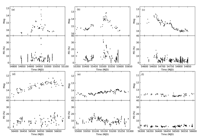
We used the data obtained with the Kanata telescope which was published in Itoh et al. (2016). The data includes -band time-series photometric and polarimetric data for 45 blazars from 2008–2014. Figure 1 shows examples of light curves and variations in the degree of polarization (PD).
Panels (a), (b), and (c) of figure 1 show examples of FSRQs: PKS 1510089 and 3C 454.3 in 2010 and in 2008, respectively. The peak-to-peak amplitudes in the light curves are large, over 2 mag in all cases, while the light curve profiles are diverse: a solitary, short flare appears in panel (a), while a number of short flares superimposed on long outbursts appear in panels (b) and (c). The light curves change their apparent characteristics year by year even for the same object, as shown in panels (b) and (c). Panels (d), (e), and (f) of figure 1 show examples of BL Lac objects: BL Lac (LBL), 3C 66A (IBL), and Mrk 501 (HBL), respectively. The peak-to-peak amplitude of the light curve in panel (d) is comparable to that of FSRQs, while the light curve profile looks different. The characterization and classification of these variations are the main subjects of this paper. The variation in polarization could give rise to some interesting features. For example, PD flares are associated with FSRQ flares, though no clear correlation can be seen in the light curve and PD variations in panels (d) and (e). Panels (e) and (f) show that the variation amplitude apparently decreases from LBL to HBL, as mentioned in the previous section.
2.2 Feature extraction with the OU process
We use the OU process for our time-series analysis. The OU process is a stochastic model based on the multivariate normal distribution whose covariance between the data at time and , , is given as:
| (1) |
where and represent the characteristic variation timescale and amplitude at , respectively (Uhlenbeck & Ornstein (1930)). For the time-series data followed by the OU process, , the observed data, , is given by , where the second term is the noise defined by the normal distribution having zero mean and variance . We can extract the characteristic features, , , and , from the observed time-series data using the OU process regression.
The time-series data introduced in § 2.1 have different observation periods for each object. The time-series data of each object was divided into one-year segments, each of which is regarded as a sample in this paper. For modeling the light curves with the OU process, the magnitude values were translated to fluxes on a logarithmic scale, simply dividing by . We assumes that the light curves are approximated with the OU process with a characteristic time-scale less than a few tens of days for our sample. The short time-scale is supported by the data in which erratic variations are detected over measurement errors in all samples. If our assumption is true, the power spectrum should be flat for frequencies () lower than the characteristic frequency, and decays as for higher frequencies (Kelly et al. (2011)). A strong linear trend in the time-series data breaks this assumption because the power becomes larger in lower frequencies. We consider that the linear trend has an origin different from the short-term variations governed by the OU process. The presence of such distinct short- and long-term variations are reported in AGN (Arévalo et al. (2006); McHardy et al. (2007); Kelly et al. (2011)) and also in blazars (Sobolewska et al. (2014)). Hence, we first subtracted the linear trend from the samples, and then performed the OU process regression. The slope value of the linear trend can be considered an indicator of the power at the lowest frequencies, and we use it as a feature for the classification in the next section.
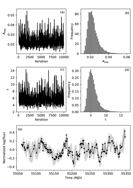
The OU process is identical to the Gaussian process with an exponential kernel. We used the python package for the Gaussian process, GPy, which includes a package for the Markov chain Monte Carlo (MCMC) method for the estimation of the posterior probability distributions of the parameters. In the present work, we estimated the posterior distribution of with a flat prior probability and that of with a positive flat prior. We fixed with a typical measurement error of the data. We estimated the posterior probability distributions of and using the MCMC method for each light-curve sample. We set . Figure 2 shows trace plots of and , their posterior distributions, and the observed and model light curves for the sample S5 0716714 between MJD 55050 and 55389. The MCMC samples converge to a stationary distribution and the posterior distributions have single-peaked profiles. In this case, we successfully obtained unique solutions of and .
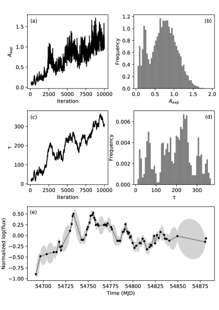
On the other hand, we found that and were not uniquely determined for several of the samples, mainly because the data size is not large enough to make a meaningful estimate of the parameters. A significant number of the samples from Itoh et al. (2016) have only data points. Even in the samples with larger data size, is not uniquely determined if it is too long. Figure 3 shows an example, AO 023516 between MJD 54617 and 54946. The MCMC samples do not converge to a stationary distribution and can be very large, reaching over 300 d. Kozłowski (2017) reports that the OU process model is degenerate when the baseline of the light-curve sample is shorter than ten times . The result in figure 3 is probably an example of such a case..
In this paper, we used only samples for which and were uniquely determined, as in figure 2. This selection reduces the number of samples to 38 for 18 objects. The selected samples include 12 samples for 8 FSRQs and 26 samples for 10 BL Lac objects. The samples are listed in table A in the Appendix. The designation of the objects to the subtypes FSRQ, LBL, IBL, and HBL is taken from Itoh et al. (2016).
Blazars occasionally exhibit large prominent flares, as shown in panel (a) of figure 1, which definitely arise from a non-stationary process, whereas the OU process model assumes a stationary stochastic process. In order to characterize the non-stationarity, we calculate the cross-validation error (CVE) using the OU process regression, as follows: First, the sample is divided into 25-d bins, a sub-sample of which is for validation while the others are for training. Then, the OU process regression is performed with the training subsets. Then, the log-likelihood is calculated from the validation subset and the optimized model. Using the other sub-samples as validation data, we obtained about log-likelihoods for each sample. The CVE is defined as their mean. A large CVE means that the validation data has a large deviation from the prediction of the model constructed from the training data. Hence, a large value of CVE indicates a high degree of non-stationarity.
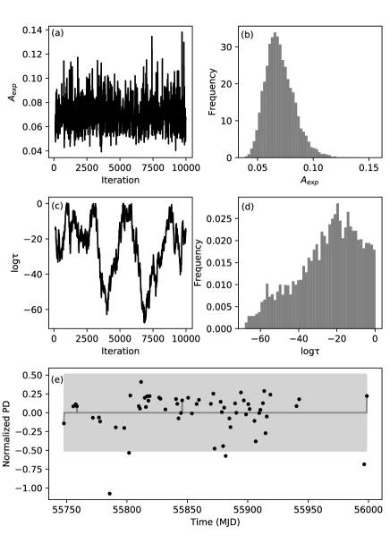
The analysis of the time-series PD data was performed in the same manner as for the light curves, that is, dividing it into one-year-segments, converting to a logarithmic scale whose linear trends were subtracted. The OU process parameter was fixed to . and were uniquely determined for the PD variations in all the samples except for seven. An example of one of the seven samples is shown in figure 4. Although, is uniquely determined, the MCMC samples of do not converge, and can be quite small (note that the scale of is logarithmic in figure 4). As a result, the model of PD is simply the mean of the data, as shown in panel (e). These results suggest that the characteristic timescale is too short to be properly determined with our data. We set for the seven samples. While a value of zero for is physically undefined, it works for training and evaluating the classifier representing very short timescales. CVEs were also calculated for the PD data. In addition, we also used the median of the PD as a feature parameter.
In total, we obtained nine features from the light curve and PD data: the four features from the light curve samples, , , the slope of the linear trend, and CVE, and five features from the PD samples, , , linear slope, CVE, and PD median. The values of the features are listed in table A in the Appendix.
2.3 Sparse multinomial logistic regression
We construct a classifier for FSRQs and BL Lac objects based on the nine features described in § 2.2. We use sparse multinomial logistic regression (SMLR) to determine the classifier (Krishnapuram et al. (2005)). We consider the problem of defining an -class classifier with labeled samples, each of which has a -dimensional feature vector, . A sample that belongs to the -th class can be expressed with a vector such that and the other elements are . Multinomial logistic regression gives the probability that a sample belongs to the -th class, as follows:
| (2) |
where is the weight vector for the -th class. The log-likelihood function is given by the data as
| (3) |
Then, the solution of SMLR is expressed as
| (4) |
where is the norm, , and is a sparsity parameter that controls the complexity of the model.
SMLR gives a linear classifier against the observed features if it is used as . In this case, SMLR can select the important features because the term makes sparse. On the other hand, a non-linear classifier can be obtained if the observed features are transformed with non-linear kernel functions. Then, we can avoid over-fitting due to the term. In the present study, the features listed in table A were normalized and the feature vector of the -th sample, , was obtained. The -th element of was obtained from and with the RBF kernel as follows:
| (5) |
where is the bandwidth.
As mentioned in § 2.2, the number of samples, , is 38. The number of classes, , is two: FSRQs and BL Lac objects. Because of the small sample size, the three subtypes LBL, IBL, and HBL are combined as one BL Lac type, while the characteristics of the subtypes are discussed in § 4.2. The classifier is evaluated from the so-called “area under the curve” (AUC), which is defined by the receiver operating characteristic (ROC) curve. The simple accuracy of the classifier is inadequate because the number of BL Lac objects is larger than that of FSRQs in our sample (12 FSRQ samples and 26 BL Lac samples). The AUC is calculated by leave-one-out cross-validation for estimating the generalization error of the classifier. Optimization of the model and the calculation of the cross-validated AUC were performed with the Java-based application SMLR111http://www.cs.duke.edu/~amink/software/smlr.
3 Results
We investigate the features that are discriminative for FSRQs and BL Lac objects based on SMLR and cross-validated AUC using the nine features obtained from the data. SMLR has two hyper-parameters, and . We first consider appropriate values for these two parameters for our study.
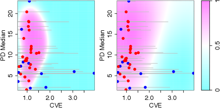
A small leads to a complicated model with a large number of samples retained in the classifier. Such a small occasionally creates an island-like boundary. Figure 5 shows examples of the probability map of BL Lac type samples calculated with (left) and (right) using two features, the light-curve CVE and PD median. We set in this case. As can be seen in the left panel, the high probability region forms an “island” within the surrounding low probability area. However, it is unlikely that the two subtypes of blazars have such a complicated boundary. A linear or slightly non-linear model, like that in the right panel, is more reasonable. We confirmed that a classifier with large bandwidths () does not have an island-like boundary using our samples. In the following analysis, we set .
The sparsity parameter, , also controls the complexity of the model. We investigated the best AUC of all combinations of the nine features against various values of . The result is given in figure 6, showing that AUC becomes maximum around . A model obtained with is too simple to appropriately classify the samples. On the other hand, a small () leads to over-fitting. We set in the following analysis.

Variables used, AUC, and accuracy of top 20 models. A bullet symbol indicates the parameter was included in that model. Light curve Polarization degree CVE Slope Median CVE Slope AUC Accuracy — — — — 0.907 0.842 — — — — 0.904 0.816 — — — 0.888 0.842 — — — 0.885 0.789 — — — 0.881 0.868 — — — 0.881 0.737 0.878 0.816 — — — 0.878 0.789 — — — 0.875 0.789 — 0.872 0.789 — — 0.872 0.816 — — 0.869 0.842 — — — — — 0.865 0.842 — 0.862 0.763 — — 0.862 0.737 — — — 0.859 0.789 — 0.856 0.763 — — 0.856 0.763 — 0.853 0.816 — — 0.853 0.789
We made an exhaustive test of all the parameters to find the most important features (e.g., Igarashi et al. (2018)). The number of combinations of the nine features is . Using SMLR, we developed 511 classifiers using models with different combinations of parameters, and calculated the AUCs for each. Table 3 lists the top 20 classifiers in the order of AUC values. For example, the classifier with the highest AUC () uses six features, that is, the CVE, , of the light curve, and the median, CVE, and of the PD. It has an accuracy of 0.842. As can be seen in the table, the correlation between the accuracy score and AUC is low in the 20 models. This is probably due to the small sample size, and indicates that a small difference in the AUC is not important. We found that CVE and of the light curve are used in all the top 20 models, and that of the light curve and PD median are used in 19 models. This result suggests that these four features are essential to classify FSRQs and BL Lac objects.
The probability of the BL Lac type () for each sample obtained with the classifier using the four parameters is listed in table A in the Appendix. We can determine the class of each sample based on . Table 3 is the error matrix for several different decision criteria: , , and . In the case of , all the samples classified as BL Lac objects are indeed BL Lac objects (Accuracy ). On the other hand, only six of the 12 FSRQs are correctly classified as FSRQ, while the other six samples are misidentified. The BL Lac prediction accuracy improves with increased decision criterion (), while the prediction accuracy of FSRQs decreases in that case. The high rate of misidentified FSRQs suggests that a significant portion of FSRQs cannot be distinguished from BL Lac objects based on the four features.
Error matrix and accuracy. Reference Accuracy Classification BL Lac FSRQ BL Lac 26 6 0.81 FSRQ 0 6 1.00 Reference Accuracy Classification BL Lac FSRQ BL Lac 25 4 0.86 FSRQ 1 8 0.89 Reference Accuracy Classification BL Lac FSRQ BL Lac 21 3 0.88 FSRQ 5 9 0.64
4 Discussion
4.1 Significance of the classifier
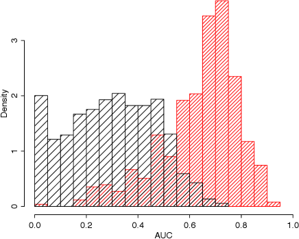
A good classifier could incidentally be obtained in high dimensional problems even if all the features are not related to the real characteristics of the samples. We tested the significance of the obtained classifier described in the previous section using artificial data sets. The sets of artificial data consist of 12 FSRQs and 26 BL Lac objects, as for the case in table A, with random values for the nine features. The random numbers were uniformly distributed between and . We made 100 sets of data and obtained AUC values, in the same manner as described in the previous section. Figure 7 shows histograms of the AUC values from the real samples (red) and from the artificial samples (black). The distribution from the real samples exhibited systematically higher AUCs than that of the random data sets. The AUC values obtained from the random data sets are concentrated in the area AUC . Thus, it is unlikely that the obtained best AUC values from the real data () are incidentally obtained.
4.2 Implications from the four features
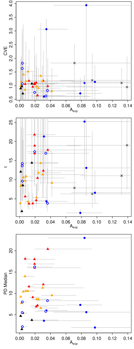
Here, we discuss the implications of the results of § 3. Figure 8 shows scatter plots of the four features. The correctly classified FSRQs () are indicated by the filled blue circles, while the misclassified FSRQs are indicated by the open circles. As can be seen from the top panel, the correctly classified FSRQs have high CVE and/or high , while the misclassified FSRQs have values for these features comparable to those of the BL Lac objects. The high value of CVE indicates the presence of prominent non-stationary flares which deviate from the stationary OU process. The high value of indicates a large amplitude of variation at the characteristic timescale, . We propose that FSRQs are characterized by rare and large flares which have a time-series structure distinct from ordinary variations. If the frequency of the flares is relatively high, a few times a year say, then the light curve can be reproduced by the OU process with a high . If the frequency is low, such as once a year, then the light curve can be divided into two distinct periods, that is, the stationary state and the non-stationary flare, which causes a high CVE. The misclassified FSRQs may be objects in which the flare frequency was so low that no flare was detected in the year.
It is not evident that the characteristics of the light-curve CVE and originate from a different structure and/or physical condition for the jets between the blazar subtypes (e.g. Itoh et al. (2016)). It is possible that it is simply due to the effect. In order to investigate this point, we analyzed the X-ray data of the HBL Mrk 421 using the X-ray light curve presented in Yamada et al. (2020). The data was obtained with XRT/Swift from 2009 to 2014. The time-interval of the X-ray light curve is 1 d. We analyzed the data in the same manner as for the optical light curves, that is, dividing it into one-year-segments, calculating the flux density in a logarithmic scale whose linear trends were subtracted, and performing the OU process regression for each segment. Table A shows the estimated CVE, , and for each sample. We successfully obtained values for the four segments listed in the table. We could not obtain those values for the segment MJD 55939–56078 mainly because of the small sample size (). The estimated values are indicated by crosses in the top and middle panels of figure 8. They are definitely in the regime of FSRQs, especially regarding the large . This result suggests that the large does not originate from different jet properties in the blazar subtypes, but from the effect.
The variation timescale of the light-curve, , was also selected as an important feature for classification. However, as shown in the middle panel of figure 8, we cannot find any clear differences between the distributions of FSRQs and BL Lac objects. This feature was selected mainly because it is useful for the classification of only one FSRQ sample, 3C 454.3 in MJD 54542–54930. This sample has a small CVE () and a not very high (), from which the object cannot be distinguished from BL Lac objects, but has an exceptionally large (). We consider that our analysis does not provide enough evidence to determine the importance of .
It is proposed that the beaming factor of FSRQs is systematically larger than that of BL Lac objects. Giommi et al. (2012) proposed that the two subtypes have a common nature, except for the beaming factor. Itoh et al. (2016) propose that the jet volume fraction occupied by the fast “spine” should be larger in FSRQs than BL Lac objects. The difference in the beaming factor would also change the characteristics of the variability. For example, a shorter variation timescale is expected with a higher beaming factor. However, our analysis provides no strong evidence that of FSRQs is systematically smaller than that of BL Lac objects, while the uncertainty of is large.
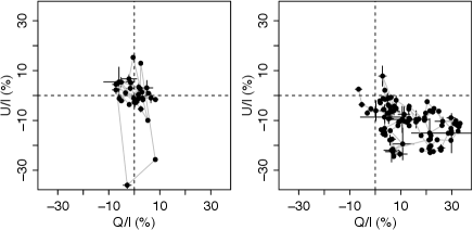
In the bottom panel of figure 8, we can see a trend that BL Lac objects have high PD medians compared with FSRQs. This characteristic is stronger when HBLs (the black triangles in the figure) are neglected. The low PD medians of HBLs are probably due to a large contamination of the unpolarized emission from their host galaxies (Shaw et al. (2013)). Figure 9 shows examples of polarization variations in the Stokes – plane. The left and right panels show the data of the FSRQ PKS 1510089 having a low PD median and that of the LBL OJ 287 having a high PD median, respectively. An increase in PD is occasionally associated with the flares of blazars, and in general the PD remains relatively low when the object is faint. In the left panel of figure 9, most of the data points exhibit low PDs, except for a few data points with high PDs over %, which are associated with the prominent flare shown in panel (a) of figure 1. The high value of the PD median in BL Lac objects indicates that PD is relatively high even in the faint state. The right panel of figure 9 shows an example: the object had a relatively high PD throughout the year. It has been proposed that the LBL object BL Lac has two polarization components: short-term variations superimposed on a stable or semi-stable component (Hagen-Thorn et al. (2002); Sakimoto et al. (2013)). The fact that the PD median was selected in our analysis suggests that the presence of a stable polarization component is a characteristic feature of BL Lac objects.
The origin of the PD median characteristic is unclear. The values of the PD median apparently correlate with in BL Lac objects, being lowest in HBLs and highest in LBLs. However, FSRQs have low PD medians, although they have the highest . Hence, the characteristic is not due to the effect, but possibly due to a difference in the jet structure between the blazar subtypes. In this case, the stable polarization component should have a different emitting site or physical condition from the short-term variations since the characteristics of the short-term flux variability can be interpreted as the effect, as discussed above. The presence of the stable component may suggest that the accelerated electrons have a long life-time with a long cooling timescale. According to Kaspi et al. (2005), the size of the broad line region (BLR) has a positive correlation with the AGN luminosity, and the AGNs with the highest luminosity have large BLRs up to sub-pc scale. FSRQs form a sub-group of blazars with the highest luminosity, not only of the jets, but also of the AGNs (Fossati et al. (1998); Shaw et al. (2013); Ghisellini et al. (2017)). The lack of a stable component in FSRQs may be reconciled with the presence of a strong radiation field induced by a large BLR causing strong Compton cooling of the electrons even in the sub-pc region, which is the source of the stable polarization component in BL Lac objects.
Giommi et al. (2012) reported that LBLs include both low luminosity FR I objects and high luminosity FR II objects. If this is the case, there may be LBLs with a low PD median. Our samples included only two LBL objects, BL Lac and OJ 287. The number of samples is so small that we cannot make conclusions about the population of LBLs. Further studies are required to understand the relationship between the presence/absence of the stable polarization component and FR types or AGN luminosity.
4.3 Features of polarization variability
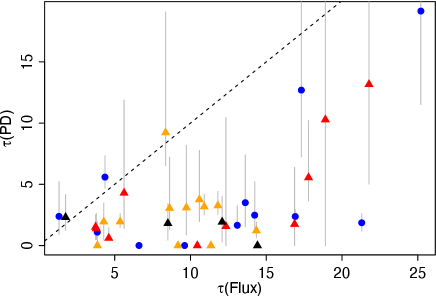
In this paper, we used features derived from both the light curves and PD variations, while the only PD feature selected as being useful for classifying FSRQs and BL Lac objects was the PD median. Figure 10 shows a scatter plot of of the light curve and of the PD variations. In this figure, we can see that the timescale of the PD variation tends to be shorter than that of the light curve. Most of the objects have a PD shorter than 5 d. As mentioned in § 2.2, the PD was too short to be uniquely determined in seven cases. These results imply that the real could be too short to be correctly estimated from our data. If this is the case, the PD features were not selected in our analysis possibly because they were not good indicators for the nature of the PD variability. The fact that the PD is significantly shorter than the light-curve suggests that the relaxation timescale of the ordered magnetic field is shorter than the cooling timescale of the accelerated electrons.
On the other hand, the presence of a stable polarization component in BL Lac objects can also cause a lack of PD variation features in the selected features. The observed Stokes parameters are a sum of those of multiple components. If the contamination of the stable component is strong, the PD variation of a flare is diluted by the stable component. For example, the increase in PD associated with a flare is canceled if the direction of polarization of the flare component is perpendicular to that of the stable component. This effect also causes the PD features to be poor indicators of the real PD variability. In future work, we will extract the features of the PD variation for both the short-term flares and the stable, or long-term, variation component by separating these components (Uemura et al. (2010)).
5 Summary
We characterized the optical variability of blazars using the OU process and investigated the features which are discriminative for the two blazar subtypes, FSRQs and BL Lac objects. Our summarized findings are as follows:
-
•
Four features, namely, the variation amplitude, , characteristic timescale, , and non-stationarity, CVE, from the light curve and the PD median are essential to classify blazars into FSRQs and BL Lac objects.
-
•
FSRQs are characterized by rare and large flares based on a large and/or CVE. We found that the X-ray variability of the HBL Mrk 421 also has large comparable to the optical variability of FSRQs. Hence, the characteristics of and CVE are governed not by the differences in the jet structure between the subtypes, but by the effect.
-
•
The high PD median of BL Lac objects suggest that they tend to have a stable polarization component. The lack of such a component in FSRQs is possibly due to strong Compton cooling from a large BLR in sub-pc scale jets.
-
•
The variation timescale of PD is significantly shorter than that of the light curves. This may indicate that the relaxation timescale of the ordered magnetic field is shorter than the cooling timescale of the accelerated electrons.
This work was supported by a Kakenhi Grant-in-Aid (No. 25120007) from the Japan Society for the Promotion of Science (JSPS).
Appendix A Samples and features
Samples and features for classification Object Start End N Light curve Polarization degree Type MJD CVE Slope Median CVE Slope () () () () S2 010922 54581 54974 69 10.55 IBL 0.86 3C 66A 54612 54974 114 10.60 IBL 0.86 3C 66A 54974 55345 142 10.40 IBL 0.85 3C 66A 55345 55671 72 14.00 IBL 0.90 3C 66A 55671 56073 30 9.20 IBL 0.85 3C 66A 56409 56797 56 7.70 IBL 0.81 S5 0716714 54665 55050 138 6.55 IBL 0.68 S5 0716714 55050 55389 156 8.65 IBL 0.83 S5 0716714 55389 55746 98 8.60 IBL 0.79 S5 0716714 55746 56125 98 9.55 IBL 0.78 S5 0716714 56484 56868 51 11.30 IBL 0.84 OJ 287 54696 55045 100 20.40 LBL 0.76 OJ 287 55045 55451 116 18.00 LBL 0.69 OJ 287 55773 56161 42 16.00 LBL 0.77 OJ 287 56488 56872 54 16.90 LBL 0.83 Mrk 421 55127 55438 36 3.75 HBL 0.61 3C 279 54621 55115 58 16.20 FSRQ 0.81 PKS 1502106 54568 55045 60 23.00 FSRQ 0.28 PKS 1510089 54759 55124 50 5.60 FSRQ 0.12 RX J1542.8612 54895 55490 99 5.50 FSRQ 0.66 PG 1553113 56629 56956 50 4.70 HBL 0.68 Mrk 501 56289 56660 84 1.60 HBL 0.59 PKS 1749096 55880 56780 77 2.00 FSRQ 0.25 3C 371 54555 54952 81 8.00 FSRQ 0.76 1ES 1959650 54577 54934 40 4.70 IBL 0.75 PKS 2155304 54628 54925 57 5.40 HBL 0.74 BL Lac 54537 54908 100 18.10 LBL 0.92 BL Lac 54908 55270 104 11.60 LBL 0.89 BL Lac 55270 55605 58 12.10 LBL 0.84 BL Lac 55605 56011 67 7.20 LBL 0.76 BL Lac 56011 56347 82 6.90 LBL 0.79 BL Lac 56347 56735 100 9.10 LBL 0.85 CTA 102 56140 56339 41 8.30 FSRQ 0.79 3C 454.3 54542 54930 108 3.60 FSRQ 0.39 3C 454.3 54930 55270 155 5.80 FSRQ 0.57 3C 454.3 55270 55795 91 7.30 FSRQ 0.48 3C 454.3 56000 56370 53 2.20 FSRQ 0.56 3C 454.3 56370 56744 78 6.00 FSRQ 0.37
Samples and features of Mrk 421. MJD N CVE 55150 55386 119 55533 55651 58 56268 56428 54 56627 56749 42
References
- Abdo et al. (2010) Abdo, A. A., Ackermann, M., Agudo, I., Ajello, M., Aller, H. D., Aller, M. F., Angelakis, E., Arkharov, A. A., et al. 2010, ApJ, 716, 30
- Angelakis et al. (2016) Angelakis, E., Hovatta, T., Blinov, D., Pavlidou, V., Kiehlmann, S., Myserlis, I., Böttcher, M., Mao, P., et al. 2016, MNRAS, 463, 3365
- Arévalo et al. (2006) Arévalo, P., Papadakis, I. E., Uttley, P., McHardy, I. M., & Brinkmann, W. 2006, MNRAS, 372, 401
- Bauer et al. (2009) Bauer, A., Baltay, C., Coppi, P., Ellman, N., Jerke, J., Rabinowitz, D., & Scalzo, R. 2009, ApJ, 699, 1732
- Baum et al. (1995) Baum, S. A., Zirbel, E. L., & O’Dea, C. P. 1995, ApJ, 451, 88
- Blandford & Königl (1979) Blandford, R. D. & Königl, A. 1979, ApJ, 232, 34
- Blandford & Rees (1978) Blandford, R. D. & Rees, M. J. 1978, in BL Lac Objects, ed. A. M. Wolfe (University of Pittsburgh Press), pp 328–341
- Fossati et al. (1998) Fossati, G., Maraschi, L., Celotti, A., Comastri, A., & Ghisellini, G. 1998, MNRAS, 299, 433
- Ghisellini et al. (1998) Ghisellini, G., Celotti, A., Fossati, G., Maraschi, L., & Comastri, A. 1998, MNRAS, 301, 451
- Ghisellini et al. (2017) Ghisellini, G., Righi, C., Costamante, L., & Tavecchio, F. 2017, MNRAS, 469, 255
- Ghisellini & Tavecchio (2008) Ghisellini, G. & Tavecchio, F. 2008, MNRAS, 387, 1669
- Ghisellini et al. (2005) Ghisellini, G., Tavecchio, F., & Chiaberge, M. 2005, A&A, 432, 401
- Giommi et al. (2012) Giommi, P., Padovani, P., Polenta, G., Turriziani, S., D’Elia, V., & Piranomonte, S. 2012, MNRAS, 420, 2899
- Hagen-Thorn et al. (2002) Hagen-Thorn, V. A., Larionova, E. G., Jorstad, S. G., Björnsson, C. I., & Larionov, V. M. 2002, A&A, 385, 55
- Hovatta et al. (2014) Hovatta, T., Pavlidou, V., King, O. G., Mahabal, A., Sesar, B., Dancikova, R., Djorgovski, S. G., Drake, A., et al. 2014, MNRAS, 439, 690
- Igarashi et al. (2018) Igarashi,Y., Takenaka, H., Nakanishi-Ohno, Y., Uemura, M., Ikeda, S., & Okada, M. 2018, Journal of the Physical Society of Japan, 87, 44802
- Ikejiri et al. (2011) Ikejiri, Y., Uemura, M., Sasada, M., Ito, R., Yamanaka, M., Sakimoto, K., Arai, A., Fukazawa, Y., et al. 2011, PASJ, 63, 639
- Itoh et al. (2016) Itoh, R., Nalewajko, K., Fukazawa, Y., Uemura, M., Tanaka, Y. T., Kawabata, K. S., Madejski, G. M., Schinzel, F. K., et al. 2016, ApJ, 833, 77
- Kaspi et al. (2005) Kaspi, S., Maoz, D., Netzer, H., Peterson, B. M., Vestergaard, M., & Jannuzi, B. T. 2005, ApJ, 629, 61
- Kelly et al. (2009) Kelly, B. C., Bechtold, J., & Siemiginowska, A. 2009, ApJ, 698, 895
- Kelly et al. (2011) Kelly, B. C., Sobolewska, M., & Siemiginowska, A. 2011, ApJ, 730, 52
- Kozłowski (2017) Kozłowski, S. 2017, A&A, 597, A128
- Krishnapuram et al. (2005) Krishnapuram, B., Carin, L., Figueiredo, M. A. T., & Hartemink, A. J. 2005, IEEE Transactions on Pattern Analysis and Machine Intelligence, 27, 957
- Marscher & Jorstad (2010) Marscher, A. P. & Jorstad, S. G. 2010, arXiv:1005.5551
- McHardy et al. (2007) McHardy, I. M., Arévalo, P., Uttley, P., Papadakis, I. E., Summons, D. P., Brinkmann, W., & Page, M. J. 2007, MNRAS, 382, 985
- Meyer et al. (2011) Meyer, E. T., Fossati, G., Georganopoulos, M., & Lister, M. L. 2011, ApJ, 740, 98
- Narayan & Yi (1995) Narayan, R. & Yi, I. 1995, ApJ, 452, 710
- Quataert (2001) Quataert, E. 2001, in Probing the Physics of Active Galactic Nuclei, ed. B. M. Peterson, R. W. Pogge, & R. S. Polidan Vol. 224 of Astronomical Society of the Pacific Conference Series (Astronomical Society of the Pacific), 71
- Ruan et al. (2012) Ruan, J. J., Anderson, S. F., MacLeod, C. L., Becker, A. C., Burnett, T. H., Davenport, J. R. A., Ivezić, Ž., Kochanek, C. S., et al. 2012, ApJ, 760, 51
- Sakimoto et al. (2013) Sakimoto, K., Uemura, M., Sasada, M., Kawabata, K. S., Fukazawa, Y., Yamanaka, M., Itoh, R., Ohsugi, T., et al. 2013, PASJ, 65, 35
- Shakura & Sunyaev (1973) Shakura, N. I. & Sunyaev, R. A. 1973, A&A, 24, 337
- Shaw et al. (2013) Shaw, M. S., Romani, R. W., Cotter, G., Healey, S. E., Michelson, P. F., Readhead, A. C. S., Richards, J. L., Max-Moerbeck, W., King, O. G., & Potter, W. J. 2013, ApJ, 764, 135
- Sobolewska et al. (2014) Sobolewska, M. A., Siemiginowska, A., Kelly, B. C., & Nalewajko, K. 2014, ApJ, 786, 143
- Stickel et al. (1991) Stickel, M., Padovani, P., Urry, C. M., Fried, J. W., & Kuehr, H. 1991, ApJ, 374, 431
- Stocke et al. (1991) Stocke, J. T., Morris, S. L., Gioia, I. M., Maccacaro, T., Schild, R., Wolter, A., Fleming, T. A., & Henry, J. P. 1991, ApJS, 76, 813
- Uemura et al. (2010) Uemura, M., Kawabata, K. S., Sasada, M., Ikejiri, Y., Sakimoto, K., Itoh, R., Yamanaka, M., Ohsugi, T., Sato, S., & Kino, M. 2010, PASJ, 62, 69
- Uhlenbeck & Ornstein (1930) Uhlenbeck, G. E. & Ornstein, L. S. 1930, Physical Review, 36, 823
- Ulrich et al. (1997) Ulrich, M.-H., Maraschi, L., & Urry, C. M. 1997, ARA&A, 35, 445
- Urry & Padovani (1995) Urry, C. M. & Padovani, P. 1995, PASP, 107, 803
- Yamada et al. (2020) Yamada, Y., Uemura, M., Itoh, R., Fukazawa, Y., Ohno, M., & Imazato, F. 2020, PASJ, in press. (arXiv:2003.08016)