Federated Graph Learning with Adaptive Importance-based Sampling
Abstract
For privacy-preserving graph learning tasks involving distributed graph datasets, federated learning (FL)-based GCN (FedGCN) training is required. A key challenge for FedGCN is scaling to large-scale graphs, which typically incurs high computation and communication costs when dealing with the explosively increasing number of neighbors. Existing graph sampling-enhanced FedGCN training approaches ignore graph structural information or dynamics of optimization, resulting in high variance and inaccurate node embeddings. To address this limitation, we propose the Federated Adaptive Importance-based Sampling (FedAIS) approach. It achieves substantial computational cost saving by focusing the limited resources on training important nodes, while reducing communication overhead via adaptive historical embedding synchronization. The proposed adaptive importance-based sampling method jointly considers the graph structural heterogeneity and the optimization dynamics to achieve optimal trade-off between efficiency and accuracy. Extensive evaluations against five state-of-the-art baselines on five real-world graph datasets show that FedAIS achieves comparable or up to 3.23% higher test accuracy, while saving communication and computation costs by 91.77% and 85.59%.
Introduction
Graph convolutional networks (GCNs) (Kipf and Welling 2016; Fey et al. 2021; Chen et al. 2018) have achieved impressing performance for a wide range of learning tasks on graph data. However, due to privacy concerns, heterogeneous subgraphs are separately stored by different data owners, constructing globally applicable GCNs requires collaborative learning. Federated graph learning (FedGL) for collaborative GCN training while preserving data privacy has attracted increasing attention (He et al. 2021; Chen et al. 2021; Liu et al. 2022). Based on the distribution of graph data, FedGL can be divided into inter-graph FedGL (He et al. 2021) and intra-graph FedGL (Chen et al. 2021). Intra-graph FedGL is common in practice e.g., in an online social application where each user has a local social network which contains interests and user interactions, and all networks form the latent complete human social network.
However, training intra-graph FedGL on large-scale heterogeneous graphs remains a challenge. Firstly, the exponentially increasing dependency of neighbor nodes over layers (i.e., neighbor explosion) causes the computation graph to be extremely large, which incurs prohibitively high computation cost. Secondly, intra-graph FedGL requires transferring intermediate embeddings across clients. This involves large number of edges connecting nodes that are stored by different clients. Since calculating embeddings for a node requires embeddings from its recursive neighbors several hops away, which could be stored by other clients, fetching neighbor embeddings across clients incurs high communication cost. Ignoring the information from neighbors across clients and treating subgraphs at various clients as independent can degrade model performance (Chen et al. 2021). Thirdly, client data in intra-graph FedGL exhibit statistical and structural heterogeneity. Different subsets of training data leads to different model accuracy and latency.
Existing methods of efficient FedGCN training can be categorized into three categories. The first category uses missing neighbor generation (Zhang et al. 2021b, a) to acquire accurate node embeddings. However, the additional training of the generative models would incur high computation and communication costs. The second category focuses on graph sampling (Zhang et al. 2021b), e.g., FedGraph (Chen et al. 2021) uses deep reinforcement learning (DRL) to select neighbor nodes for embedding aggregation. However, it ignores the graph structural heterogeneity information, resulting in inaccurate node embeddings and large variance in the gradients. The third category periodically transfer cross-client neighbor embedding transmission (Chen et al. 2021; Zhang et al. 2022; Deng et al. 2023) to reduce communication costs. However, it fails to capture the dynamics of model training to determine the optimal transfer period, resulting in inferior model performance. As for graph sampling for centralized learning, there are three types: 1) node-wise sampling methods iteratively sample a number of neighbor nodes for each node (Hamilton et al. 2017; Dai et al. 2018); 2) layer-wise sampling methods select a number of nodes for each GCN layer (Chen et al. 2018; Zou et al. 2019); and 3) subgraph sampling methods sample a number of subgraphs from each training batch (Chiang et al. 2019; Zeng et al. 2019). However, since these approaches are not designed for FL, they require access to potentially sensitive raw data which risk privacy of local clients. Besides, such methods neglect communication costs and would incur substantial communication burden when the volume of the graph data is large.
To address these limitations, we propose a novel federated graph sampling scheme - the Federated Adaptive Importance-based Sampling (FedAIS) approach for large-scale graph data node classification tasks. It reduces the graph sampling variance and achieves substantial cost savings by efficiently leveraging historical embedding estimators and focuses the limited communication and computation resources on training important local samples. By designing an adaptive embedding synchronization scheme, it is capable of achieving the optimal trade-off between test accuracy and computation and communication cost savings. The key advantages of FedAIS are summarized as follows.
-
•
Scalability: FedAIS is able to scale FedGCN to large graphs with a constant memory cost with respect to input node sizes. For a selected set of batches, FedAIS prunes the GCN computation graph so that only nodes inside the current batches and their direct 1-hop cross-client neighbors are retained, regardless of the depth of the GCN. Historical embeddings are used to accurately fill in the inter-dependency information of cross-client neighbors.
-
•
Efficiency: FedAIS achieves highly efficient FedGL and reduces unnecessary sample training via dynamic importance-based sampling that considers both structural information and optimization dynamics. It reduces cross-client neighbor embedding communication through adaptive embedding synchronization to select the optimal transmission interval that achieves the fast decay of the objective function.
-
•
Convergence: FedAIS ensures that the global model converges in an efficient manner. Theoretical analyses show that the approximation variance induced by importance-based node sampling and the staleness of historical embedding is upper bounded.
We evaluate FedAIS on five graph datasets of different scales under real-world workloads. Compared to the five state-of-the-art approaches, FedAIS achieves significant cost savings when training FedGCN models with thousands of FL participants. On average, it achieves comparable or up to 3.23% higher test accuracy, while incurring 91.77% and 85.59% lower communication and lower computation cost, respectively. In this way, FedAIS achieves significantly more advantageous trade-offs between efficiency and accuracy compared to existing approaches.
Related Work
FedGCN Training
Existing work on efficient intra-graph FedGCN training on large graphs can be divided into three branches. The first branch uses missing neighbor generation to obtain accurate node embeddings (Zhang et al. 2021b, a). However, it only focuses on improving prediction accuracy without considering the computation and communication overhead caused by additional training of the generative model. The second branch focuses on graph sampling approaches (Zhang et al. 2021b), e.g., FedGraph (Chen et al. 2021) uses deep reinforcement learning (DRL) to select neighbor nodes for embedding aggregation. However, since it ignores the graph topology and heterogeneity of clients, it results in inaccurate node embeddings and large variance in the gradients. Besides, it would incur large computation overhead as each local client needs to separately train two additional DRL networks. The third branch periodically transfer cross-client neighbor node embeddings to reduce communication costs (Chen et al. 2021; Du and Wu 2022; Zhang et al. 2022; Deng et al. 2023). However, they fail to capture the dynamics of model training to determine the optimal transfer period, resulting in inferior model performance.
Sampling-based GCN Training
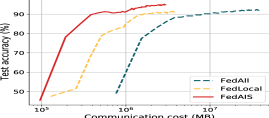
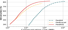
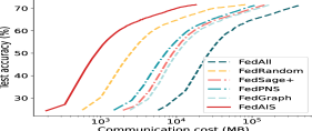
One approach to scaling up GCN training is graph sampling, which can be categorized into: 1) node-wise sampling, 2) layer-wise sampling, and 3) subgraph sampling. Node-wise sampling methods (Hamilton et al. 2017; Cong et al. 2020) iteratively sample a number of neighbors for each node based on specific probabilities (e.g., calculated based on node centrality). Layer-wise sampling methods (Chen et al. 2018; Zou et al. 2019) independently sample a number of nodes for each GCN layer. Since multiple nodes are jointly sampled in each layer, the time cost of the sampling process is reduced by avoiding the exponential extension of neighbors. However, since nodes of different layers are sampled independently, some sampled nodes may have no connections with the ones in the previous layer, which would deteriorate the training performance. Subgraph sampling methods (Chiang et al. 2019; Zeng et al. 2019) sample a number of subgraphs for each batch in GCN training. However, graph partitioning of large graphs is time-consuming and the model performance is highly sensitive to the cluster size. Those three categories of methods, however, require direct access to data features, which would risk privacy leakage of local clients in FL settings. Besides, those methods neglect communication costs and would incur substantial communication costs when the volume of the graph data is large. Thus, we propose FedAIS to improve trade-offs between accuracy and efficiency (Fig. 1). Here, FedLocal is the federated GraghSage (Hamilton et al. 2017), which conducts random selection of within-client neighbor nodes, where the cross-client neighbor information is ignored. FedPNS performs periodic selection of both within-client and cross-client neighbor nodes.
Problem Formulation
There are two types of entities involved: a server , and clients . Each client owns a graph dataset , where is an undirected graph with vertices, edges. is the total number of all clients’ local data samples. We focus on the task of node classification, where each vertex is associated with a feature vector and a label . Given a -layer FedGCN, let , denote loss functions of an individual sample and all samples on client ’s local model. denotes the loss function of the global model. We formulate FedGCN learning as a distributed optimization problem:
| (1) |
where the -th graph convolution layer embedding of node is defined as:
| (2) |
Here, is the activation function. denotes the set of neighbor nodes of and . Suppose the average degree in a local graph is . To calculate of node in an -layer FedGCN, on average the number of neighbors involved is (Chen et al. 2017), which results in an exponential increase in computation and communication overhead with respect to . Thus, local clients cannot afford to calculate all embedding terms which need to be computed and transmitted recursively. Aggregating only within-client neighbor embeddings while ignoring cross-client information leads to inferior model performance (Chen et al. 2021).
Our FedAIS Approach
Joint Analysis of Variance and Overhead
To construct a global FedGCN model with fast convergence speed and low prediction error, we need to first analyze the sources of variances and biases when applying graph sampling strategies. Existing graph sampling approaches suffer from high variances and biases introduced to the stochastic gradients due to the approximation of node embeddings at different layers (Cong et al. 2020; Du and Wu 2022). We denote as the embedding approximation of node in the -th layer. Specifically, the variance of stochastic gradient estimator , can be decomposed as:
| (3) |
denotes the variance of estimated gradients to their exact values , resulting from the inner layer embedding approximation in forward propagation. The term denotes the variance of mini-batch gradients to the full gradients due to the mini-batch sampling.
Assumption 1.
Let be differentiable and -Lipschitz smooth and the value of be bounded by a scalar .
Theorem 1.
Under Assumption 1, if for all and all , the final output error of layer in training round is bounded by:
| (4) |
Theorem 1 lets us immediately derive an upper error bound for the estimated gradients, i.e.,
| (5) |
From the decomposition of variance in Eq. (3) and the upper error bound for the estimated gradients in Eq. (5), we conclude that any graph sampling method introduces two sources of variance (i.e., the embedding approximation variance and the stochastic gradient variance). Therefore, to accelerate model convergence and reduce computation and communication overhead, both kinds of variance needs to be accounted in designing a graph sampling strategy.
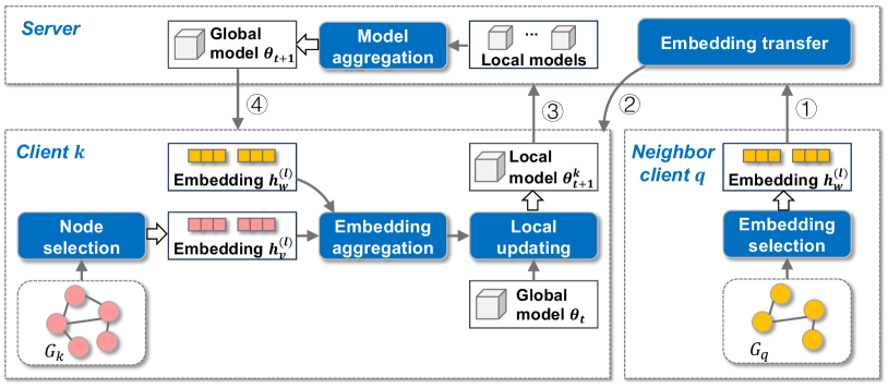
System Overview
FedAIS consists of two modules (as shown in Fig. 2).
-
1.
Historical Embedding-based Graph Sampling. In training round , client updates the importance scores of its local training samples based on historical embeddings and training losses of individual samples. Then, client selects its most influential samples to be used for FedGCN model training. Using historical embeddings and training losses helps reduce both embedding approximation variance and stochastic gradient variance, thereby enabling accurate FedGCN model training.
-
2.
Adaptive Embedding Synchronization and Model Updating. With the influence estimation and sampling results, each client updates its historical embeddings and performs node aggregation. Then, it updates its local model and estimates the next optimal synchronization interval via the joint analysis of the overhead and error-convergence. Finally, client sends the updated local model to the server, which then aggregates the local models to produce the global model.
Historical Embedding-based Graph Sampling
While evaluating embedding , it is prohibitively costly to calculate all terms since they need to be computed and transmitted recursively (i.e., we again need the embeddings of all ’s neighbor nodes ). To reduce computation and communication costs, we introduce the historical embedding for FedGCN as an affordable approximation.
| (6) |
Here, we separate the within-client neighbors into two parts: 1) within-client in-batch nodes , which are part of the current batch ; and 2) within-client out-of-batch nodes , which are part of the client but not included in the current batch . For both neighbor nodes, we approximate their embeddings via historical embeddings acquired in previous iterations. Compared to the previous approach which incurs exponentially computation and communication costs, that incurred by historical embedding estimator increases linear with , i.e., computation operations and communication cost, where and are numbers of global training rounds and local training epochs.
Based on the historical embedding estimator and the variance analysis, we select training nodes that contribute most to the objective function and accelerate model convergence. It can be casted into the following optimization problem,
| (7) |
The most straightforward solution is to use the norm of gradient as the probability. However, it requires the calculation of derivatives for each client at each local epoch , which is computationally prohibitive (Li et al. 2021). To solve this issue, we instead use the difference of training losses between two consecutive local model updates to approximate the gradient . Then, client calculates the probability by normalizing the differences across its all training samples,
| (8) |
Thus, the computational complexity is since client only requires one forward propagation.
Adaptive Embedding Synchronization
To analyze the effect of on the expected runtime, we consider the following delay model. In round , the time taken by client to conduct a local model update at the -th epoch is modeled as a random variable and the total communication delay is a random variable . Then, the communication cost is , where is the average network bandwidth during round . For the full synchronization, the total time to complete each round is , while for the periodic synchronization, the average time to complete each round is where . Consider the simplest case where and are constants, and is the ratio of communication delay to computation cost, which depends on the size of FedGCN model, network bandwidth and client computing capacity, etc.
Assumption 2.
The stochastic gradient evaluated on the mini-batch with bounded variance, , where .
Theorem 2.
From the optimization error bound in Eq. (9), the error-runtime trade-off for different synchronization communication intervals can be derived. While a larger reduces the runtime per iteration and makes the first term in Eq. (9) smaller, it also adds noise and increases the last term.
Then, we determine the optimal embedding synchronization interval to minimize the optimization error for each training batch. We start with infrequent cross-client embedding synchronization for improved convergence speed, and gradually transiting to higher embedding synchronization frequencies to reduce the prediction error of the learned global model. Specifically, at each training round , the server selects the optimal embedding transmission interval that achieves the fast test loss decay of the global model for the next interval. Theorem 2 illustrates that there is an optimal value that minimizes the optimization error bound at round between the server and all selected clients,
| (10) |
It can be observed from Eq. (10) that the generated synchronization period sequence decreases along with the objective value on the test set when the learning rate is fixed. It is consistent with the intuition that the trade-off between error-convergence and overhead varies over time. Compared to the initial training phase, the benefit of using a large synchronization interval diminishes as the model converge since a lower error is preferred in the latter training phase. In some scenarios where the Lipschitz constant and the gradient variance bound are unknown and estimating these constants are difficult due to the highly non-convex and high-dimensional loss surface. As an alternative, we propose a simpler rule where we approximate by 0, and divide Eq. (10) by to obtain the basic synchronization interval,
| (11) |
where is the ceil function to round to the nearest integer. In practical implementations, we take the test loss as the objective function value and the average batch number as the initial synchronization period , both of which can be easily obtained during training.
Implementation
The proposed FedAIS is illustrated in Algorithm 1. Specifically, in the -th global round, the server randomly selects a set of clients, and distributes the current model to them (Lines 4-6). Each selected client calculates the loss for each sample and updates its selection probability (Lines 11-12). Then, during each local epoch , client selects a batch of samples with . For each layer of FedGCN, when the number of local batch training epoch satisfies , client firstly calculates with Eq. (6) by aggregating embeddings of both within-client neighbors and cross-client neighbors. Then, it performs embedding synchronization by asking neighbor client to update the selected cross-client neighbor embeddings and transmit them back (Lines 13-18). Then, client updates its local model and sends to the server. The server aggregates updates by conducting model aggregation and updating interval (Lines 7-8). In this way, the server and clients collaboratively train a FedGCN model with high prediction accuracy and low overhead.
Convergence Analysis
Without loss of generality, we analyze an arbitrary interval sequence with synchronization iterations.
Theorem 3.
(Convergence of FedAIS) Suppose the learning rate remains the same as ,
| (12) |
The global model is guaranteed to converge to:
| (13) |
The key idea of proof is as follows. To understand the condition (12), we consider the case when is a constant. Then, the converge condition is identical to that for mini-batch SGD: . Provided that the sequence of communication periods is bounded, the learning rate in mini-batch SGD can be easily adjusted to satisfy condition (12). Specifically, when the communication period sequence decreases, the last two terms in (12) become easier to satisfy, and the differences between the objective values of two consecutive rounds are bounded. The full proof of FedAIS convergence is presented in Appendix.
Experiment Evaluation
Experimental Settings
| Dataset | Coauthor | Pubmed | Yelp | Amazon2M | |
|---|---|---|---|---|---|
| 18,333 | 19,717 | 716,847 | 232,965 | 2,449,029 | |
| 163,788 | 88,648 | 13,954,819 | 114,615,892 | 61,859,140 | |
| # features | 6,805 | 500 | 300 | 602 | 100 |
| # classes | 15 | 3 | 100 | 41 | 47 |
| Train/ Val/ Test | 0.8/ 0.1/ 0.1 | 0.8/ 0.1/ 0.1 | 0.75/ 0.10/ 0.15 | 0.66/ 0.10/ 0.24 | 0.8/ 0.1/ 0.1 |
| 100 clients | |||||
| 146 | 158 | 5,376 | 1,538 | 19,592 | |
| 173 | 879 | 138,815 | 1,140,985 | 610,748 | |
| 1,030 | 747 | 73,230 | 517,533 | 784,277 | |
| Method | Metric | Performance results (%) standard deviations | |||||||||
| Coauthor | Pubmed | Yelp | Amazon2M | ||||||||
| iid | non-iid | iid | non-iid | iid | non-iid | iid | non-iid | iid | non-iid | ||
| FedAll | testAcc | 89.98 0.78 | 84.46 1.08 | 87.74 2.16 | 86.42 1.07 | 91.57 1.29 | 89.69 2.08 | 82.38 0.61 | 81.66 0.62 | 71.46 1.03 | 67.89 0.82 |
| F1-score | 78.38 1.25 | 73.03 1.13 | 85.62 0.87 | 84.51 0.91 | 29.03 1.14 | 27.71 1.41 | 76.34 1.12 | 74.89 1.15 | 29.89 0.85 | 25.82 0.79 | |
| AUC | 92.35 1.32 | 75.26 1.28 | 96.14 0.14 | 96.03 0.74 | 75.45 2.03 | 73.36 1.83 | 95.54 0.05 | 92.41 1.02 | 83.62 0.65 | 60.12 0.87 | |
| FedRandom | testAcc | 87.09 0.78 | 81.53 1.28 | 87.16 2.16 | 84.92 1.07 | 92.25 2.29 | 86.79 1.12 | 79.34 0.52 | 77.52 0.91 | 71.78 0.49 | 65.45 0.64 |
| F1-score | 72.95 1.05 | 68.13 2.13 | 83.62 0.87 | 81.32 0.91 | 29.61 2.14 | 27.21 1.41 | 72.34 1.52 | 70.56 1.05 | 30.54 0.68 | 24.43 0.48 | |
| AUC | 88.58 1.27 | 70.76 0.82 | 96.12 0.16 | 92.06 0.74 | 74.84 2.03 | 71.58 0.79 | 93.66 0.05 | 88.42 1.08 | 83.16 0.54 | 56.98 1.12 | |
| FedSage+ | testAcc | 85.02 0.78 | 81.95 1.03 | 86.82 1.16 | 85.08 1.14 | 83.45 0.79 | 82.79 0.43 | 78.34 0.28 | 74.52 0.62 | 71.47 0.79 | 66.42 0.81 |
| F1-score | 76.78 1.05 | 54.93 0.63 | 84.62 0.87 | 83.21 0.91 | 30.12 0.74 | 29.84 0.81 | 76.54 0.97 | 66.56 1.05 | 29.89 0.38 | 27.38 0.37 | |
| AUC | 89.29 1.17 | 74.45 0.92 | 90.83 0.58 | 89.06 0.49 | 71.26 1.03 | 72.27 0.72 | 94.76 0.55 | 92.42 1.18 | 83.62 0.48 | 58.24 0.42 | |
| FedPNS | testAcc | 87.03 0.21 | 81.65 0.93 | 87.38 1.23 | 85.87 1.05 | 90.92 0.59 | 85.97 0.82 | 82.25 1.26 | 80.24 0.73 | 71.36 0.78 | 66.74 0.43 |
| F1-score | 72.58 2.34 | 68.32 1.62 | 85.96 2.74 | 84.81 2.46 | 28.99 1.02 | 28.01 1.24 | 76.10 0.62 | 73.63 0.62 | 29.63 0.78 | 25.95 1.07 | |
| AUC | 87.69 2.37 | 72.81 1.72 | 95.87 1.29 | 93.86 1.09 | 75.22 0.25 | 73.74 1.02 | 95.07 1.28 | 91.12 0.36 | 83.39 0.52 | 58.19 0.62 | |
| FedGraph | testAcc | 88.09 1.06 | 83.18 1.25 | 87.82 0.97 | 85.17 0.84 | 90.98 0.82 | 87.41 0.58 | 82.18 0.75 | 80.12 1.14 | 71.75 0.62 | 66.93 0.47 |
| F1-score | 73.19 1.24 | 68.03 1.86 | 85.69 1.04 | 83.58 1.41 | 31.39 1.22 | 29.16 1.02 | 75.88 0.83 | 71.42 1.04 | 30.21 0.82 | 25.43 0.93 | |
| AUC | 88.85 0.78 | 72.15 1.43 | 95.89 1.62 | 93.97 1.27 | 77.75 0.51 | 73.31 0.89 | 94.96 1.17 | 92.61 0.72 | 82.82 0.78 | 59.89 0.53 | |
| FedAIS | testAcc | 88.12 0.12 | 85.49 0.79 | 88.36 0.59 | 85.26 1.07 | 94.12 0.17 | 91.13 0.72 | 82.48 0.18 | 81.84 0.93 | 71.84 0.31 | 67.99 0.58 |
| F1-score | 74.86 1.07 | 69.16 0.37 | 86.34 0.21 | 83.72 0.83 | 31.65 0.26 | 30.87 0.69 | 76.16 0.23 | 74.69 0.53 | 30.84 0.52 | 27.52 0.81 | |
| AUC | 92.52 0.12 | 73.75 1.04 | 95.97 0.31 | 96.28 0.94 | 79.96 0.12 | 74.35 0.72 | 95.26 1.05 | 92.47 0.82 | 84.16 0.26 | 60.72 0.43 | |
Implementation. We implemented FedAIS and deployed it in an FL system consisting of one server and 100 clients. To further investigate the performance of FedAIS in large-scale FL systems, we also tested it in an environment with up to 1,000 clients. Our implementation is based on Python 3.11 and Pytorch Geometric 2.0.1 (Fey and Lenssen 2019). All the experiments are performed on Ubuntu 20.04 operating system equipped with a 32-core AMD Ryzen Threadripper PRO 5965WX @ 3.800GHz CPU, 192G of RAM and a NVIDIA RTX A5000 GPU with 24GB memory.
Datasets and Models. We use five real-world graph datasets of different scales, i.e., Coauthor (Shchur et al. 2018), Pubmed (Sen et al. 2008), Yelp (Zeng et al. 2019), Reddit (Hamilton et al. 2017), Amazon2M (Hu et al. 2020). We partition training/ validation sets over 100 clients in both independent and identically distributed (iid) setting and non-iid setting. We use a non-iid partition by , with a Dirichlet distribution and allocate a ratio of instances of class to client (Li et al. 2022; Yurochkin et al. 2019). Since the original graph is extremely dense, we downsample the edges in local subgraphs by 50% (Hamilton et al. 2017). The test dataset is located at the server and the statistics of the datasets are presented in Table 1. We use the widely adopted GraphSage model (Hamilton et al. 2017) with FedAvg to construct FedGCN models: FedAuthor, FedPubmed, FedYelp, FedReddit, FedAmazon (Hu et al. 2020). Each model has two hidden layers with 256, 128 neurons. We set the ratio of sample selection to 0.7, the number of neighbors sampled to 10, and the minimum embedding synchronization interval to 2 batch training epochs. We use Adam as the optimizer with the weight decay 0.001 and ReLU as the activation function. We set the learning rate , the fixed batch number is 10, and the global warm-up round is 1. We conduct training until a pre-specified test accuracy is reached, or a maximum number of iterations has elapsed (e.g., 100 rounds). We perform 5-fold cross validation and report the average results.
Comparison Baselines. 1) FedAll: It conducts training using all local samples and performs random neighbor node selection of both local subgraph neighbors and cross-client neighbors. 2) FedRandom: It performs random selection for both local samples and neighbor nodes in each batch training. 3) FedSage+ (Zhang et al. 2021b): It proposes a GNN-based neighbor generative model for each client to predict the features of each node’s cross-client neighbors. 4) FedPNS (Du and Wu 2022): It conducts training using all local samples and conducts periodic neighbor node selection for cross-client neighbor nodes. We set the periodic interval to 2 local batch training epochs. 5) FedGraph (Chen et al. 2021): It performs FL training using all local samples and selects local subgraph neighbors and cross-client neighbors by adjusting sampling policies based on DRL.
Results and Discussions
FedAIS achieves comparable or higher accuracy. We adopt three metrics (Falessi et al. 2021; Herbold et al. 2018), i.e., test accuracy, F1-score, and area under the curve (AUC), to evaluate the accuracy of FedGCN models. We compare FedAIS with other baseline methods by training different FedGCN models in both iid and non-iid settings. We present the results of those accuracy metric scores and the standard deviations of the final global models in Table 2. It shows that FedAIS achieves test accuracy, F1 score, and AUC scores that are comparable to or better than other methods. For example, for model FedYelp trained on Yelp dataset in the iid setting, the test accuracy of FedAIS is 4.55%, 3.87%, 5.20%, 5.14 higher than other methods, respectively.
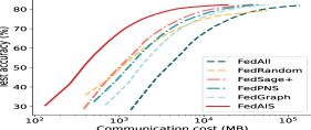
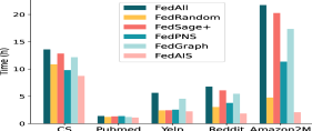
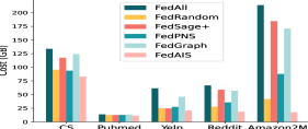
FedAIS significantly saves computation and communication costs. We present the test accuracy with the size of communication cost for training FedReddit and FedAmazon in iid settings in Fig. 4. The test accuracy, F1-score and AUC scores with the size of communication cost for training FedAuthor, FedPubmed and FedYelp in both iid and non-iid settings are much similar to that in Fig. 4. The results in Fig. 4 show that FedAIS requires much less amount of communication volume than the other baselines to achieve the target test accuracy, which leads to less computation time for transmitting those node embedding bytes and updating model parameters. Besides, we present the total computation and communication overhead for training FedGCN models in Fig. 4. It shows that FedAIS achieves significantly savings of both computation and communication costs than other baselines.
Ablation Study
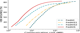
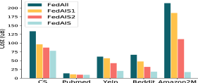
We perform ablation studies to show the effectiveness of each component of FedAIS. We compare FedAIS against the following ablation baselines: 1) FedAll; 2) FedAIS1: it only conducts the proposed dynamic importance sampling method of local samples without adaptive embedding synchronization; 3) FedAIS2: it conducts training using all local samples with the proposed adaptive embedding synchronization. We present the test accuracy with the size of communication cost and the total communication costs in Fig. 6. The results show that FedAIS, FedAIS1 and FedAIS2 achieve higher performance in saving much communication costs to reach the target accuracy scores and FedAIS performs the best among them. Thus, both the dynamic importance sampling module and the adaptive embedding synchronization module are effective to construct FedAIS.
Sensitivity Analysis
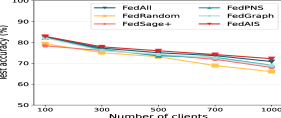
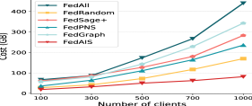
Impact of the number of clients. We conduct experiments with different numbers of clients engagement, i.e., . We present the test accuracy and communication cost of the model FedReddit trained with different number of clients in Fig. 6. It shows that the test accuracy of FedAIS is consistently high, i.e., above 75.0%, as the number of client increases to 1,000, and achieves test accuracy that is comparable to or higher than others. Besides, it shows that communication costs increase as the number of clients increases and FedAIS achieves substantial cost savings than other baselines in all settings.
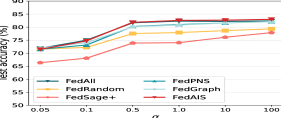
Impact of the non-iid degree. We present the test accuracy of the model FedReddit with different non-iid degrees, i.e., , in Fig. 7(a). It shows that FedAIS achieves accuracy scores that are comparable to or higher than other baselines. Besides, these accuracy scores increase as increases, and when is greater than 0.5, the accuracy scores are relative high. The accuracy scores with the sizes of communication cost for training the model FedReddit with different non-iid degrees are much similar to that in Fig. 3(a), which shows that FedAIS consistently requires less communication cost than others.
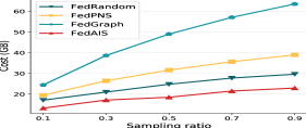
Impact of the ratio of samples selected. Fig. 7 presents the test accuracy and communication costs of the model FedReddit when the selection ratio is 0.1, 0.3, 0.5, 0.7, 0.9. Here, we adjust FedPNS and FedGraph so that they can select corresponding ratios of nodes. It shows that both the test accuracy and communication cost increase as the sampling ratio increases and FedAIS performs much better. Besides, due to the large size of the Reddit dataset, FedAIS can construct a FedGCN model with high test accuracy and less communication cost by sampling only 0.1 proportion of local samples, which achieves significantly more advantageous trade-offs between accuracy and efficiency.
Conclusions
In this paper, we proposed a federated adaptive importance-based sampling approach, FedAIS, for large-scale graph data in node classification tasks. It achieves substantial computation and communication costs by efficiently utilizing historical embedding estimators and reducing unnecessary sample training via dynamic importance-based sampling. Besides, it reduces cross-client neighbor embedding communication through adaptive embedding synchronization. In this way, FedAIS determines the optimal communication period and achieves faster convergence with lower costs and lower prediction errors. Extensive evaluations show that FedAIS achieves comparable or higher test accuracy, while saving significant communication and computation costs.
References
- Chen et al. (2021) Fahao Chen, Peng Li, Toshiaki Miyazaki, and Celimuge Wu. Fedgraph: Federated graph learning with intelligent sampling. IEEE Transactions on Parallel and Distributed Systems, 33(8):1775–1786, 2021.
- Chen et al. (2017) Jianfei Chen, Jun Zhu, and Le Song. Stochastic training of graph convolutional networks with variance reduction. arXiv preprint arXiv:1710.10568, 2017.
- Chen et al. (2018) Jie Chen, Tengfei Ma, and Cao Xiao. Fastgcn: fast learning with graph convolutional networks via importance sampling. arXiv preprint arXiv:1801.10247, 2018.
- Chiang et al. (2019) Wei-Lin Chiang, Xuanqing Liu, Si Si, Yang Li, Samy Bengio, and Cho-Jui Hsieh. Cluster-gcn: An efficient algorithm for training deep and large graph convolutional networks. In Proceedings of the 25th ACM SIGKDD international conference on knowledge discovery & data mining, pages 257–266, 2019.
- Cong et al. (2020) Weilin Cong, Rana Forsati, Mahmut Kandemir, and Mehrdad Mahdavi. Minimal variance sampling with provable guarantees for fast training of graph neural networks. In Proceedings of the 26th ACM SIGKDD International Conference on Knowledge Discovery & Data Mining, pages 1393–1403, 2020.
- Dai et al. (2018) Hanjun Dai, Zornitsa Kozareva, Bo Dai, Alex Smola, and Le Song. Learning steady-states of iterative algorithms over graphs. In International conference on machine learning, pages 1106–1114. PMLR, 2018.
- Deng et al. (2023) Pan Deng, Xuefeng Liu, Jianwei Niu, and Chunming Hu. Graphfed: A personalized subgraph federated learning framework for non-iid graphs. In 2023 IEEE 20th International Conference on Mobile Ad Hoc and Smart Systems (MASS), pages 227–233. IEEE, 2023.
- Du and Wu (2022) Bingqian Du and Chuan Wu. Federated graph learning with periodic neighbour sampling. In 2022 IEEE/ACM 30th International Symposium on Quality of Service (IWQoS), pages 1–10. IEEE, 2022.
- Falessi et al. (2021) Davide Falessi, Aalok Ahluwalia, and Massimiliano DI Penta. The impact of dormant defects on defect prediction: A study of 19 apache projects. ACM Transactions on Software Engineering and Methodology (TOSEM), 31(1):1–26, 2021.
- Fey and Lenssen (2019) Matthias Fey and Jan E. Lenssen. Fast graph representation learning with PyTorch Geometric. In ICLR Workshop on Representation Learning on Graphs and Manifolds, 2019.
- Fey et al. (2021) Matthias Fey, Jan E Lenssen, Frank Weichert, and Jure Leskovec. Gnnautoscale: Scalable and expressive graph neural networks via historical embeddings. In ICML, pages 3294–3304. PMLR, 2021.
- Hamilton et al. (2017) Will Hamilton, Zhitao Ying, and Jure Leskovec. Inductive representation learning on large graphs. Advances in neural information processing systems, 30, 2017.
- He et al. (2021) Chaoyang He, Keshav Balasubramanian, Lichao Sun, Lifang He, Liangwei Yang, Philip S Yu, Yu Rong, et al. Fedgraphnn: A federated learning system and benchmark for graph neural networks. arXiv preprint arXiv:2104.07145, 2021.
- Herbold et al. (2018) Steffen Herbold, Alexander Trautsch, and Jens Grabowski. A comparative study to benchmark cross-project defect prediction approaches. In Proceedings of the 40th International Conference on Software Engineering, pages 1063–1063, 2018.
- Hu et al. (2020) Weihua Hu, Matthias Fey, Marinka Zitnik, Yuxiao Dong, Hongyu Ren, Bowen Liu, Michele Catasta, and Jure Leskovec. Open graph benchmark: Datasets for machine learning on graphs. Advances in neural information processing systems, 33:22118–22133, 2020.
- Kipf and Welling (2016) Thomas N Kipf and Max Welling. Semi-supervised classification with graph convolutional networks. arXiv preprint arXiv:1609.02907, 2016.
- Li et al. (2021) Anran Li, Lan Zhang, Juntao Tan, Yaxuan Qin, Junhao Wang, and Xiang-Yang Li. Sample-level data selection for federated learning. In IEEE INFOCOM 2021-IEEE Conference on Computer Communications, pages 1–10. IEEE, 2021.
- Li et al. (2022) Qinbin Li, Yiqun Diao, Quan Chen, and Bingsheng He. Federated learning on non-iid data silos: An experimental study. In 2022 IEEE 38th International Conference on Data Engineering (ICDE), pages 965–978. IEEE, 2022.
- Liu et al. (2022) Rui Liu, Pengwei Xing, Zichao Deng, Anran Li, Cuntai Guan, and Han Yu. Federated graph neural networks: Overview, techniques and challenges. arXiv preprint arXiv:2202.07256, 2022.
- Sen et al. (2008) Prithviraj Sen, Galileo Namata, Mustafa Bilgic, Lise Getoor, Brian Galligher, and Tina Eliassi-Rad. Collective classification in network data. AI magazine, 29(3):93–93, 2008.
- Shchur et al. (2018) Oleksandr Shchur, Maximilian Mumme, Aleksandar Bojchevski, and Stephan Günnemann. Pitfalls of graph neural network evaluation. arXiv preprint arXiv:1811.05868, 2018.
- Yurochkin et al. (2019) Mikhail Yurochkin, Mayank Agarwal, Soumya Ghosh, Kristjan Greenewald, Nghia Hoang, and Yasaman Khazaeni. Bayesian nonparametric federated learning of neural networks. In International conference on machine learning, pages 7252–7261. PMLR, 2019.
- Zeng et al. (2019) Hanqing Zeng, Hongkuan Zhou, Ajitesh Srivastava, Rajgopal Kannan, and Viktor Prasanna. Graphsaint: Graph sampling based inductive learning method. arXiv preprint arXiv:1907.04931, 2019.
- Zhang et al. (2021a) Chenhan Zhang, Shuyu Zhang, JQ James, and Shui Yu. Fastgnn: A topological information protected federated learning approach for traffic speed forecasting. IEEE Transactions on Industrial Informatics, 17(12):8464–8474, 2021a.
- Zhang et al. (2021b) Ke Zhang, Carl Yang, Xiaoxiao Li, Lichao Sun, and Siu Ming Yiu. Subgraph federated learning with missing neighbor generation. Advances in Neural Information Processing Systems, 34:6671–6682, 2021b.
- Zhang et al. (2022) Taolin Zhang, Chuan Chen, Yaomin Chang, Lin Shu, and Zibin Zheng. Fedego: Privacy-preserving personalized federated graph learning with ego-graphs. arXiv preprint arXiv:2208.13685, 2022.
- Zou et al. (2019) Difan Zou, Ziniu Hu, Yewen Wang, Song Jiang, Yizhou Sun, and Quanquan Gu. Layer-dependent importance sampling for training deep and large graph convolutional networks. Advances in neural information processing systems, 32, 2019.