Federated PAC-Bayesian Learning on Non-IID data
Abstract
Existing research has either adapted the Probably Approximately Correct (PAC) Bayesian framework for federated learning (FL) or used information-theoretic PAC-Bayesian bounds while introducing their theorems, but few considering the non-IID challenges in FL. Our work presents the first non-vacuous federated PAC-Bayesian bound tailored for non-IID local data. This bound assumes unique prior knowledge for each client and variable aggregation weights. We also introduce an objective function and an innovative Gibbs-based algorithm for the optimization of the derived bound. The results are validated on real-world datasets.
Index Terms— Federated learning, PAC-Bayesian framework, generalization error
1 Introduction
To address privacy concerns in distributed learning, federated learning (FL) has emerged as a viable solution, enabling multiple local clients to collaboratively train a model while retaining their private data and without sharing it [1, 2]. However, in real-world scenarios, data across different devices is not identically and independently distributed (non-IID), which poses challenges in model training and convergence [3].
Significant efforts have been made to improve performance and analyze convergence in non-IID FL [4], but few have provided theoretical guarantees by establishing generalization bounds. Most existing FL generalization analyses rely on the Probably Approximately Correct (PAC) Bayesian theory, first formulated by McAllester [5, 6]. Building on the McAllester’s bound, these analyses typically compute local bounds or apply existing PAC-Bayesian bounds directly, overlooking the non-IID nature of FL. This approach is flawed, as the PAC-Bayesian framework assumes that each data point is IID, ignoring non-IID data and directly employing the PAC-Bayesian theory, which potentially results in inaccurate or overly relaxed bounds. Consequently, techniques developed for the PAC-Bayesian framework are not directly applicable to non-IID FL. Therefore, this work aims to advance the theoretical underpinnings of non-IID FL.
Related works. The PAC-Bayesian framework has been extensively researched in recent years [7, 8, 9], yielding tighter and non-vacuous bounds. However, there has been limited exploration in the context of FL. Some studies have proposed information theoretic-based PAC-Bayesian bounds using Rate-distortion theory to prove generalization bounds [10, 11], providing an information-theoretic perspective on enhancing generalization capacity. Others have followed McAllester’s approach, attempting to directly apply the FL paradigm to the bound. For example, the authors in [12, 13] applied McAllester’s bound in a multi-step FL scenario; Omni-Fedge [14] used the PAC-Bayesian learning framework to construct a weighted sum objective function with a penalty, considering only a local client bound instead of the entire system, which precludes obtaining global information; and FedPAC [15] employed PAC learning to balance utility, privacy, and efficiency in FL. However, these approaches do not account for the non-IIDness of FL.
Our contributions. First, we derive a federated PAC-Bayesian learning bound for non-IID local data, providing a unified perspective on federated learning paradigms. To the best of our knowledge, this is the first non-vacuous bound for a model averaging FL framework. Specifically, due to the non-IID nature of clients, we assume that each client has unique prior knowledge rather than a common one. Additionally, the aggregation weights for non-IID clients vary instead of being uniform. Based on the derived bound, we define an objective function that can be computed by each local client rather than on the server and propose a Gibbs-based algorithm dubbed FedPB for its optimization. This algorithm not only preserves the privacy of each client but also enhances efficiency. Finally, we validate our proposed bounds and algorithm on two real-world datasets, demonstrating the effectiveness of our bounds and algorithm.
2 Problem Setting
In this section, we introduce the federated PAC-Bayesian learning setting. The whole system comprises clients, each equipped with its own dataset consisting of IID data points. Here denotes the input space and denotes the output space. Each dataset is presumed to be drawn from an unknown data generating distribution . Moreover, let be a given loss function and is a stochastic estimator on client where is the hypothesis class. In the PAC-Bayesian framework, each client holds a tailored prior distribution . The objective of each client is to furnish a posterior distribution , where denotes the set of distributions over . We then define the population risk:
| (1) |
and the empirical risk:
| (2) |
by averaging over the posterior distribution of each client. In federated learning, each client will upload their posterior distributions to a central server, and then the server will aggregate the transmitted model in a weighted manner:
where and are the global prior and posterior, respectively, and the averaging weight be a probability distribution on . For the sake of generality, we can assume that and . For intuition of this aggregation, we can see that minimizing the weighted objective function is actually equivalent to maximizing the logarithm of the corresponding posterior: In addition, we denote the Kullback-Leibler (KL) divergence as if and otherwise.
3 Main theorem
In this section, we will present our novel bounds on the non-IID FL scenario.
Theorem 1 (Federated PAC-Bayesian learning bound).
For any , assume the loss function is bounded in , the following inequality holds uniformly for all posterior distributions and for any ,
| (3) |
Proof.
Let the local generalization error: , then the global generalization error: . For any and , applying the Hoeffding’s lemma to , we have that, for each client ,
Since each may come from different . i.e., non-IID, we cannot directly plug this result to the PAC-Bayesian bound. Note that for each client , is independent of , we have that
And we apply Donsker and Varadhan’s variational formula [16] for to get:
| (4) |
Recall the definition of the global generalization error:
and note that . Applying the Chernoff bound:
Let , that is, . Thus, plug this into the above result we have that
Therefore, we prove the statement by leveraging the complement of the probability. ∎
The RHS of Equation 3 comprises two components: the empirical term and the complexity term. Note that our bound eschews the typical smoothness and convexity assumptions on the loss often made by other FL frameworks. Moreover, an intuition can be presented for Equation 3 that the bound will be tighter with the increasing of clients scales, which is further corroborated by the evaluation in Section 5.3.
Corollary 1 (The choice of ).
Suppose and denotes the cardinality of a set. For any and a properly chosen , with probability at least ,
| (5) |
Proof.
Equation 5 generally offers a strategy for selecting the value of parameter so that the complexity term can be minimized.
4 FedPB: Optimize the upper bound
We denote . Consider the following local objective function:
| (6) |
In our methodology, we introduce FedPB for a general scenario. It comprises two phases, designed to iteratively optimize the priors and posteriors for each client. Notably, in contrast to previous studies, clients are not required to upload their private prior and posterior distributions to the server, ensuring their privacy.
Phase 1 (Optimize the posterior). Given a fixed parameter and the prior during the training epoch , we aim to optimize the posterior as yielding the solution:
Phase 2 (Optimize the prior). Having derived the optimal posterior , the prior can be updated by since it minimizes .
Link with personalized federated learning. Since the prior and is equal to the aggregated global posterior at epoch , the prior can be viewed as the global knowledge. Optimizing the objective function (6) minimizes the disparity between the global and local knowledge, which is a a prevalent personalization strategy in FL [17].
Re-parameterization trick. Utilizing the Bayesian neural network [18] as the local model aligns with our setting where all parameters are random, and we are optimizing their posterior distribution. In particular, the prior and posterior are defined as follows:
with every model parameter being independent. Computing the Gibbs posterior directly can be challenging, hence we select the gradient descent as an alternative way. The update rule of (6) at round is:
where the parameter can be regarded as the learning rate of the GD and the KL-divergence is the regularization term. Calculating the gradients and directly can be intricate, but the re-parameterization trick is capable of tackling this issue. Concretely, we translate the to and then compute the deterministic function , where signifies an element-wise multiplication. As a result, we have , indicating its computability using an end-to-end framework with back-propagation.
5 Evaluation
In this section, we demonstrate our algorithm and our theoretical arguments with the FL non-IID setting. Specifically, the aggregation weight is defined as the sample ratio of client relative to the entire data size across all clients. For the global aggregation, the global mean and covariance are calculated by and , respectively. Furthermore, we utilize two real-world datasets: MedMNIST (medical image analysis) [19] and CIFAR-10 [20]. For each dataset, we adopt three distinct data-generating approaches for local clients: 1) Balanced: each client holds an equal number of samples; 2) Unbalanced: varying sample counts per client (e.g., for 10 clients); 3) Dirichlet: differing sample counts per client following a Dirichlet distribution [21]. Besides, the entire FL system encompasses clients, initializing their posterior models uniformly from a global posterior model.
Additionally, we deploy two versions of Bayesian neural networks: one with 2 convolutional layers for MedMNIST and another with 3 layers for CIFAR-10. The CrossEntropy loss serves as our loss function, and it is optimized by the Adam optimizer [22] with a learning rate of 1e-3.
5.1 Bound evaluation
To validate our bounds, we set the confidence bound on . Our evaluation underscores a correlation between the generalization error and the complexity, emphasizing the tightness of our bound. Fig. 1 illustrates an initial increase in the generalization error and a concurrent decrease in complexity during the early stages of the training process, attributed to empirical loss optimization. Subsequently, as neural network training advances, the KL-divergence stabilizes. Throughout this progression, we can observe that the generalization error is consistently bounded by the complexity value.
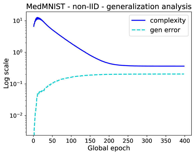
(a) Gen. for MedMNIST
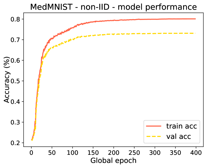
(b) Acc. for MedMNIST
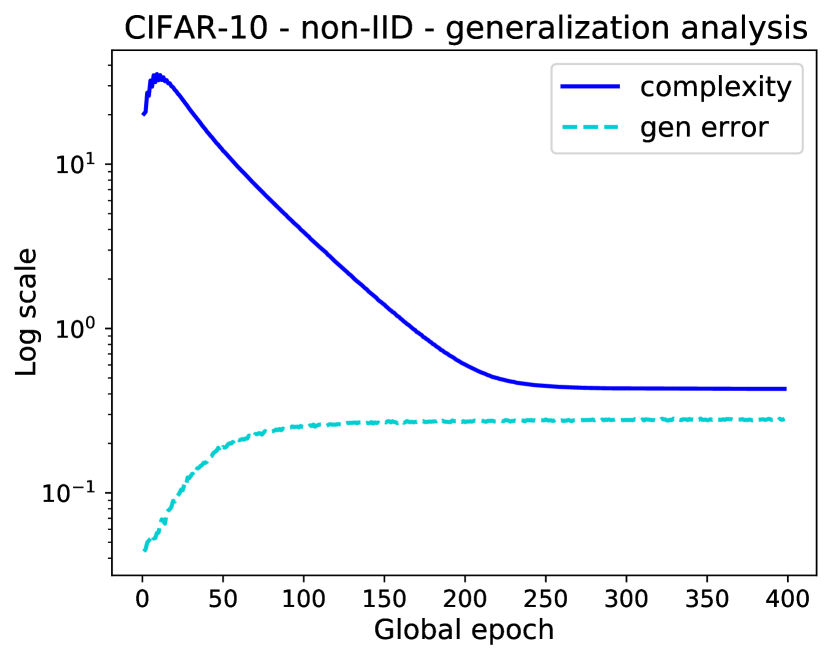
(c) Gen. for CIFAR-10
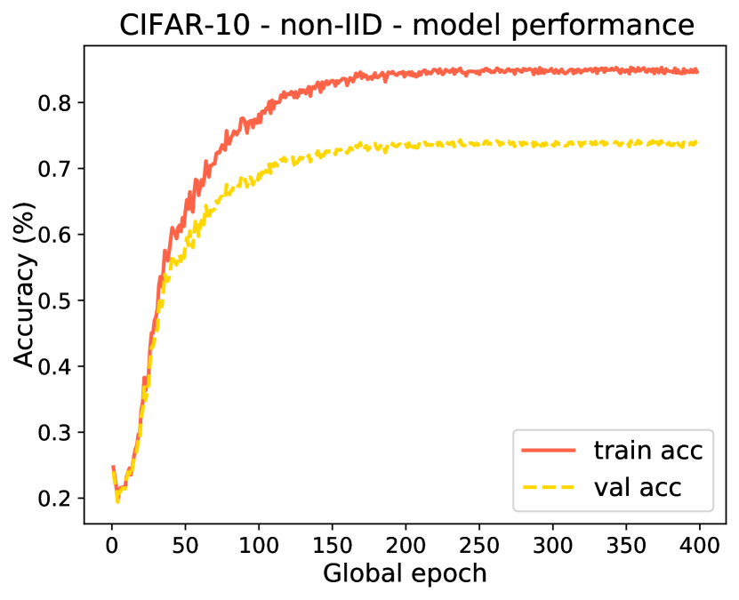
(d) Acc. for CIFAR-10
5.2 Data-dependent prior
Here, we preform the ablation study of data-dependent (trainable) prior compared with data-independent (fixed, chosen before training) prior and report the mean ± standard deviation (std) accuracy of the global model in Table 1, evaluated over multiple experimental seeds. The results demonstrate the superior efficacy of the data-dependent strategy over both datasets across all three scenarios. This superiority arises from the data-dependent prior’s ability to harness more global knowledge, combined with its adaptability during training.
| Method | MedMNIST | CIFAR10 | ||||||
|---|---|---|---|---|---|---|---|---|
| Balanced | Unbalanced | Dirichlet | Balanced | Unbalanced | Dirichlet | |||
|
||||||||
|
||||||||
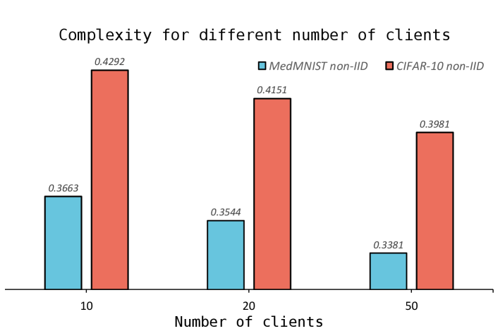
5.3 Different client scales
Lastly, we assess the influence of varying client scales on our complexity bounds. As depicted in Fig. 2, in the evaluation of both datasets with the Dirichlet generating method, by increasing the number of clients from 10 to 20 and 50, we observe a consistent decrease in the value of complexity. This observation aligns with our analysis in Equation 3.
References
- [1] Brendan McMahan, Eider Moore, Daniel Ramage, Seth Hampson, and Blaise Aguera y Arcas, “Communication-efficient learning of deep networks from decentralized data,” in Artificial intelligence and statistics. PMLR, 2017, pp. 1273–1282.
- [2] Zihao Zhao, Yuzhu Mao, Yang Liu, Linqi Song, Ye Ouyang, Xinlei Chen, and Wenbo Ding, “Towards efficient communications in federated learning: A contemporary survey,” Journal of the Franklin Institute, 2023.
- [3] Yue Zhao, Meng Li, Liangzhen Lai, Naveen Suda, Damon Civin, and Vikas Chandra, “Federated learning with non-iid data,” arXiv preprint arXiv:1806.00582, 2018.
- [4] Xiang Li, Kaixuan Huang, Wenhao Yang, Shusen Wang, and Zhihua Zhang, “On the convergence of fedavg on non-iid data,” arXiv preprint arXiv:1907.02189, 2019.
- [5] David A McAllester, “Some pac-bayesian theorems,” in Proceedings of the eleventh annual conference on Computational learning theory, 1998, pp. 230–234.
- [6] David A McAllester, “Pac-bayesian model averaging,” in Proceedings of the twelfth annual conference on Computational learning theory, 1999, pp. 164–170.
- [7] Matthias Seeger, “Pac-bayesian generalisation error bounds for gaussian process classification,” Journal of machine learning research, vol. 3, no. Oct, pp. 233–269, 2002.
- [8] Olivier Catoni, “Pac-bayesian supervised classification: the thermodynamics of statistical learning,” arXiv preprint arXiv:0712.0248, 2007.
- [9] Luca Oneto, Michele Donini, Massimiliano Pontil, and John Shawe-Taylor, “Randomized learning and generalization of fair and private classifiers: From pac-bayes to stability and differential privacy,” Neurocomputing, vol. 416, pp. 231–243, 2020.
- [10] Milad Sefidgaran, Romain Chor, and Abdellatif Zaidi, “Rate-distortion theoretic bounds on generalization error for distributed learning,” Advances in Neural Information Processing Systems, vol. 35, pp. 19687–19702, 2022.
- [11] LP Barnes, Alex Dytso, and H Vincent Poor, “Improved information theoretic generalization bounds for distributed and federated learning,” in 2022 IEEE International Symposium on Information Theory (ISIT). IEEE, 2022, pp. 1465–1470.
- [12] Milad Sefidgaran, Romain Chor, Abdellatif Zaidi, and Yijun Wan, “Federated learning you may communicate less often!,” arXiv preprint arXiv:2306.05862, 2023.
- [13] Romain Chor, Milad Sefidgaran, and Abdellatif Zaidi, “More communication does not result in smaller generalization error in federated learning,” arXiv preprint arXiv:2304.12216, 2023.
- [14] Sai Anuroop Kesanapalli and BN Bharath, “Federated algorithm with bayesian approach: Omni-fedge,” in ICASSP 2021-2021 IEEE International Conference on Acoustics, Speech and Signal Processing (ICASSP). IEEE, 2021, pp. 3075–3079.
- [15] Xiaojin Zhang, Anbu Huang, Lixin Fan, Kai Chen, and Qiang Yang, “Probably approximately correct federated learning,” arXiv preprint arXiv:2304.04641, 2023.
- [16] Monroe D Donsker and SR Srinivasa Varadhan, “On a variational formula for the principal eigenvalue for operators with maximum principle,” Proceedings of the National Academy of Sciences, vol. 72, no. 3, pp. 780–783, 1975.
- [17] Xu Zhang, Yinchuan Li, Wenpeng Li, Kaiyang Guo, and Yunfeng Shao, “Personalized federated learning via variational bayesian inference,” in International Conference on Machine Learning. PMLR, 2022, pp. 26293–26310.
- [18] Jost Tobias Springenberg, Aaron Klein, Stefan Falkner, and Frank Hutter, “Bayesian optimization with robust bayesian neural networks,” Advances in neural information processing systems, vol. 29, 2016.
- [19] Jiancheng Yang, Rui Shi, and Bingbing Ni, “Medmnist classification decathlon: A lightweight automl benchmark for medical image analysis,” in IEEE 18th International Symposium on Biomedical Imaging (ISBI), 2021, pp. 191–195.
- [20] Alex Krizhevsky, Geoffrey Hinton, et al., “Learning multiple layers of features from tiny images,” 2009.
- [21] Mikhail Yurochkin, Mayank Agarwal, Soumya Ghosh, Kristjan Greenewald, Nghia Hoang, and Yasaman Khazaeni, “Bayesian nonparametric federated learning of neural networks,” in International conference on machine learning. PMLR, 2019, pp. 7252–7261.
- [22] Diederik P Kingma and Jimmy Ba, “Adam: A method for stochastic optimization,” arXiv preprint arXiv:1412.6980, 2014.