FEM on nonuniform meshes for nonlocal Laplacian: Semi-analytic Implementation in One Dimension
Abstract.
In this paper, we compute stiffness matrix of the nonlocal Laplacian discretized by the piecewise linear finite element on nonuniform meshes, and implement the FEM in the Fourier transformed domain. We derive useful integral expressions of the entries that allow us to explicitly or semi-analytically evaluate the entries for various interaction kernels. Moreover, the limiting cases of the nonlocal stiffness matrix when the interactional radius or automatically lead to integer and fractional FEM stiffness matrices, respectively, and the FEM discretisation is intrinsically compatible. We conduct ample numerical experiments to study and predict some of its properties and test on different types of nonlocal problems. To the best of our knowledge, such a semi-analytic approach has not been explored in literature even in the one-dimensional case.
Key words and phrases:
Finite element method, nonlocal operator, nonuniform meshes, nonlocal stiffness matrix, nonlocal Allen-Cahn equation2Corresponding author. School of Mathematics, Shanghai University of Finance and Economics, Shanghai, 200433, China. The research of the author is partially supported by the National Natural Science Foundation of China (Nos. 12201385 and 12271365) and the Fundamental Research Funds for the Central Universities (No: 2021110474). Email: ctsheng@sufe.edu.cn (C. Sheng).
3Division of Mathematical Sciences, School of Physical and Mathematical Sciences, Nanyang Technological University (NTU), 637371, Singapore. The research of the author is partially supported by Singapore MOE AcRF Tier 2 Grants: MOE2018-T2-1-059 and MOE2017-T2-2-144. Email: lilian@ntu.edu.sg (L.-L. Wang).
1. Introduction
We consider the following nonlocal constrained value problem on a nonzero measure volume:
| (1.1) |
where the nonlocal operator is defined as
| (1.2) |
where is called a horizon parameter and the kernel is a nonnegative, radial function (i.e., for any ), compactly supported in , and has a bounded second moment. It is known that nonlocal models (1.1) provides an alternative way to modeling many phenomena and complex systems in diverse fields, for instance, the materials science with crack nucleation and growth, fracture, and failure of composites [5], the peridynamics model for mechanics [9, 28, 36], and nonlocal heat conduction [12]. We also refer to the up-to-date review paper [12, 15, 18] and the monograph [14] for more detail.
There has been much interest in developing numerical algorithms for nonlocal models, particularly for PDEs involving the integral fractional Laplacian, which can be viewed as a limiting case of the nonlocal operator [17, 38], i.e., The recent works on PDEs involving integral fractional Laplacian operator particularly include finite difference methods [16, 22, 23], finite element methods [2, 3], and spectral methods [31, 33, 35]. The interested readers may also refer to [7, 18, 27] for three up-to-date review papers. It should be noted that finite element method in frequency domain space for integral fractional Laplacian is provided in [10, 29, 34], where the entries of the stiffness matrix can provide exact form in one dimension, and can be simply expressed as one-dimensional integral on a finite interval in two dimension. This fact encourages us to try to extend this method for more general problems involving the nonlocal operator (1.2).
Besides, extensive numerical results have been conducted on various kinds nonlocal models. Chen and Gunzburger [9] provided a systematic study of algorithmic and implementation issues using continuous and discontinuous Galerkin finite element methods for peridynamics model. Tian and Du [37] introduce a finite element and quadrature-based finite difference scheme, compare the similarities and differences of the nonlocal stiffness matrices for the two methods, and study fundamental numerical analysis issues. Wang and Tian [32] develop a fast and faithful collocation method for a two-dimensional nonlocal diffusion model. Liu, Cheng and Wang [28] introduced and analyzed a fast Galerkin and adaptive Galerkin finite element methods to solve a steady-state peridynamic model. Additionally, other numerical methods for nonlocal models have been proposed, including the finite difference method [40], the finite element methods [24, 6], the collocation methods [25, 21, 30, 8], and so on. The development of the aforementioned methods relies on constructing specific quadrature formulas to discretize the underlying nonlocal operators, which unavoidably introduces truncation errors. However, these truncation errors often hinder our ability to analyze the attractive structure of the nonlocal stiffness matrices and affect the numerical stability of our solver on some extreme meshes, e.g., graded and geometric meshes. Recently, Li, Liu, and Wang [26] developed an efficient Hermite spectral-Galerkin method for nonlocal diffusion equations in unbounded domains, where the derivation therein was built upon the convolution property of the Hermite functions.
In this paper, we provide a semi-analytic means for computing the piecewise linear FEM stiffness matrix for nonlocal problem (1.1). Then, we can obtain an explicit form of the one-dimensional integral for the entries of the stiffness matrix without generating any truncation errors. This one-dimensional integral can even be evaluated exactly for most of the kernel functions, such as the fractional kernel , with the normalized constant and the index . Note that such an integral representation is derived from (i) implementation of FEM in the Fourier transformed domain, and (ii) use of some analytic formulas in the handbook [1, 11] to evaluation of the inner integral. Benefit from this explicit expression, we show the two limiting cases of the nonlocal stiffness matrix: (a) when , it reduces to the stiffness matrix associated with the classical Laplacian operator , see (2.33), and (b) when , it becomes the stiffness matrix corresponding to the integral fractional Laplacian operator . As a byproduct, we numerically predicted the condition number of the nonlocal stiffness matrix (even for some extreme mesh) behaves like , where and denote the maximum and minimum of the mesh size, and denotes the number of meshes. Our approach is suitable for wider range of nonlocal interaction kernel on the uniform and nonuniform meshes. Numerical experiments show that our scheme is asymptotically compatible scheme [37]. Note that we only focus on one dimensional problems in this work to better illustrate the idea. The multidimensional generalizations are possible and will be carried out in separate works.
The rest of this paper is organized as follows. In section 2, we present a piecewise linear finite element method on nonuniform and uniform meshes for model problem (1.1), and derive the explicit integral form for the entries of the nonlocal stiffness matrix. In section 3, ample numerical results for nonlocal problems with various both regular and singular kernels, including accuracy testing, limiting behaviors, eigenvalue problem and nonlocal Allen-Cahn equation, are presented to show the efficiency and accuracy. Finally, we give some concluding remarks and discussions in the last section.
2. Finite Element Method in Fourier Domain
Following the same notation as in [36], we introduce the energy space
| (2.1) |
equipped with the semi-norm
| (2.2) |
and the norm
| (2.3) |
We further define the constrained energy space as
| (2.4) |
The bilinear form on and the inner product on is, respectively, denoted by
| (2.5) |
Then, the weak formulation of (1.1) is to find such that
| (2.6) |
In this section, we compute the nonlocal FEM stiffness matrix. To fix the idea, we focus on the piecewise linear FEM with the partition:
| (2.7) |
and the piecewise linear finite element basis:
| (2.8) |
for Correspondingly, we have the FE approximation space:
Then the FE approximation to (1.1) is to find such that
| (2.9) |
where is the standard piecewise linear interpolation of on . We write
and obtain the following linear system of (2.9):
where is the nonlocal FEM stiffness matrix with entries given by
| (2.10) |
and
2.1. FEM nonlocal stiffness matrix
Through the implementation in the Fourier transformed domain, we can derive the following exact integral formulas for computing the stiffness matrix.
Theorem 2.1.
Let
| (2.11) |
and define
| (2.12) |
Then the stiffness matrix can be evaluated by the component-wise integral
| (2.13) |
where the matrix-valued function with the entries given by
| (2.14) |
Here, means the function performs component-wisely upon the matrix .
Proof.
Let be the zero extension of on to . Then by [10, Lemma 2.1], its Fourier transform is
| (2.15) | ||||
where
Using Parseval identity and the translation property: , we derive from (2.8), (2.10) and (2.15) that
| (2.16) |
Using (2.15), we obtain from direct calculation that
| (2.17) |
where
| (2.18) |
Using the trigonometric identities
| (2.19) |
we obtain from (2.14) and (2.18) readily that
| (2.20) |
where we denote
One verifies readily that for Thus, we derive from integration by parts that
| (2.21) |
Recall the sine integral formula (see [11, P. 427]):
| (2.22) |
Inserting (2.20) into (2.21), we find from (2.22) immediately that
| (2.23) |
Then we obtain from (2.16)-(2.17) and (2.23) that
| (2.24) |
This completes the proof. ∎
Theorem 2.1 is valid for the interaction radius The bandwidth of the stiffness matrix increases as increases, which becomes full as It is known that the nonlocal operator (1.2) tend to integral fractional Laplacian as when the corresponding kernel function is chosen to satisfy
| (2.25) |
where denotes the characteristic (indicator) function of and
| (2.26) |
Theorem 2.2 (Case II: ).
With the interchange in the order of integration in the above proof, we can derive the nonlocal stiffness matrix for
Theorem 2.3.
Proof.
Note that when , we have is independent of . Recall the integral formula (cf. [19, (3.12)]): for any , we have
| (2.30) |
We change the order of integration in the last equality of (2.16), and derive from (2.30) that
| (2.31) |
which is identical to the FEM stiffness matrix derived in [10, Theorem 1] with the formula given in (2.30). ∎
The above explicit formula allows for the exact evaluation or accurate computation of the stiffness matrix for general interaction kernel function and study the intrinsic properties of this matrix.
2.2. FEM nonlocal stiffness matrix with
To study the compatibility to the usual FEM stiffness matrix, when , we consider the special case with
| (2.32) |
where is chosen so that it satisfies the second moment condition: We derive from the formulas in Theorem 2.1 straightforwardly the following interesting identity, which leads to the usual FEM stiffness matrix when
Corollary 2.1.
Under (2.32), we have the identity
| (2.33) |
where is the usual FEM stiffness matrix for on with that is,
Consequently, we have
Proof.
As we can simplify in (2.12) and evaluate (2.14) directly to derive
Direct calculation using (2.13) shows that is a penta-diagonal symmetric matrix with the nonzero entries on the main diagonal and two upper off-diagonals given by
Together with (2.13), we can obtain the explicit form of stiffness matrix for given nonlocal interaction kernels, e.g., the following nonlocal interaction kernels
| (2.34) |
where is chosen to satisfy the normalization
Then we have Thus for given in (2.32), we find
| (2.35) |
by direct calculaton, we can obtain the identity (2.33). ∎
Remark 2.1.
Theorem 2.4.
Proof.
In this case, , then we have
| (2.38) |
where
| (2.39) |
This completes the proof. ∎
| (2.40) |
2.3. Nonlocal FEM stiffness matrix on uniform meshes
As a special case of Theorem 2.1, the nonlocal stiffness matrix of FEM on uniform meshes reduces to a symmetric Toeplitz matrix.
Theorem 2.5.
Given a uniform partition with , the nonlocal stiffness matrix is a symmetric Toeplitz matrix of the form
| (2.41) |
i.e., Here, the generating vector can be evaluated by
| (2.42) |
where and
| (2.43) |
with the constants , and
Proof.
In this case, the entries in (2.14) can be simplified into
where we observed from the definition (2.12) that is an even function in for fixed and also noted that the symmetric properties of coefficients and summation in Thus we can denote
which implies the entries on each diagonal are the same, i.e., is a symmetric Toeplitz matrix, so is The expression (2.51)-(2.52) is a direct consequence of (2.12)-(2.13).
Remark 2.3.
For any and fixed integer in (2.52) has the following piecewise representation:
-
(i)
If then we have
(2.44) and
(2.45) -
(ii)
If then we have
(2.46)
Case II (): Consider the following fractional Laplacian kernel
with and in the Gamma function. Then we have
| (2.47) |
where
| (2.48) |
Correspondingly, we define piecewise linear FEM basis associated with uniform partition
| (2.49) |
According to (2.13), we can easily obtain the entries of the nonlocal stiffness matrix on uniform mesh, which enjoys the Toeplitz structure.
Corollary 2.2.
For uniform partition , the nonlocal stiffness matrix is a symmetric Toeplitz matrix given by
| (2.50) |
is generated by the vector in the first row or column of with
| (2.51) |
where
| (2.52) |
and the constants .
Proof.
One can follow the same procedure as in the proof of Theorem 2.1 to obtain the desired result. ∎
Proposition 2.1.
For any and fixed integer in (2.52) has the following piecewise representation:
-
(i)
If then we have
(2.53) and
(2.54) -
(ii)
If then we have
(2.55)
Remark 2.4.
We observe from (2.51) that the bandwidth of the above matrix (2.50) is directly determined by the ratio of , which plays an important role in studying the sparsity properties of the stiffness matrix. A particular case is when and the fractional interaction kernels (2.36), we can derive the explicit form of the entries
| (2.56) |
which implies that as the matrix in (2.56) reduces to the usual (tri-diagonal) FEM stiffness matrix .
Remark 2.5.
Denote , then we can obtain the explicit form of stiffness matrix for given fractional interaction kernels (2.36)
| (2.57) |
3. Numerical Studies and Discussions
In this section, we first conduct a numerical study of the conditioning of the stiffness matrix on three sets of typical non-uniform grids used in practice to resolve singular solutions. We then numerically solve several types of nonlocal problems by using the FEM nonlocal matrix to show the efficiency and accuracy of the proposed scheme.
-
•
Two sets of typical non-uniform grids: graded & Geometric (can show the advantage of exact computation)!
-
•
Numerical results include (i) accuracy test; (ii) the use of non-uniform grids
3.1. Conditioning of the stiffness matrix on nonuniform meshes
An issue of interest is the condition number estimation for the FEM nonlocal stiffness matrix. It is a well-studied topic in the uniform meshes case, but much less known in this nonuniform meshes setting. In general, the mesh geometry affects not only the approximation error of the finite element solution but also the spectral properties of the corresponding stiffness matrix.
Extensive research has been conducted on the condition number of the nonlocal stiffness matrix on uniform grids (cf. [4, 42]), which the entries of the nonlocal stiffness matrix can be computed exactly based on the definition of hypersingular integrals form therein. With the aid of the analytical expressions, the following condition number bounds for uniform mesh were reported in [42, p.1772]:
| (3.1) |
However, the study on the condition number of the nonlocal stiffness matrix on the non-uniform mesh is still open. Inspired by the result of the condition number for FEM stiffness on nonuniform mesh in [20, (26)], we predict the condition number of FEM stiffness matrix (2.13) on nonuniform meshes associated with fractional kernel (2.32) is
| (3.2) |
where and . It is clear that the above prediction can reduce to the result with uniform mesh (3.1) when .
We will explore this numerically on graded, geometric and Shishkin meshes in order to demonstrate the prediction or conjecture. In the following numerical experiment, we will choose the mesh division as follows:
-
(i)
Graded meshes: A graded meshes on the interval is defined as follows
(3.3) From (3.2), the condition number of FEM stiffness matrix on the above graded meshes is
(3.4) -
(ii)
Geometric meshes: A geometric meshes on the interval is defined according to
(3.5) where (, is independent of ) is subdivision ratio.
Using (3.2), the condition number of FEM stiffness matrix on the above geometric meshes is
(3.6) -
(iii)
Shishkin meshes: A Shishkin meshes is piecewise uniform mesh over with elements. For , we refer to the mesh size over and as and to the mesh size over as .
According to (3.2), the condition number of FEM stiffness matrix on the above Shishkin meshes is
| (3.7) |
In Figure 3.1 (a)-(c), we plot the condition number of the stiffness matrix against various , fixed horizon and different . We observe a good agreement between the numerical results and (3.2), which indicates a clear dependence of the condition number on three parameters: the mesh ratio , the size of the nonlocality horizon parameter , and index of the fractional kernel function .
(a) .
(b) .
(c) .
(d) .
Meanwhile, we plot the first smallest eigenvalue of the stiffness matrix against various and different in Figure 3.1 (d), where we observed that the smallest eigenvalue of satisfy
This result is consistent with the classical usual Laplacian (i.e., ) and the integral fractional Laplacian (i.e., ) (cf. [10]).
3.1.1. Diagonal dominance
The study of diagonal dominance of the stiffness matrix has been a research subject of a longstanding interest in numerical linear algebra and numerical analysis. The diagonal dominance property of the stiffness matrix associated with fractional Laplacian operators has been proved in [29], which can be viewed as a limiting case of this paper (cf. [15, 17, 38]). In what follows, we restrict our attention to the uniform meshes case and discuss the intrinsic property of the stiffness matrix as , that is, we extended the following diagonal dominance property of the stiffness matrix when .
Theorem 3.6.
For , the FEM stiffness matrix associated with fractional kernel function (2.36) on uniform meshes is diagonally dominant and off-diagonal entries are negative.
Proof.
For , let , then . From (2.56), we have
| (3.8) |
Define
For , we can easily obtain and
It knows that is a symmetric Toeplitz matrix from Corollary 2.1 and is a five-diagonal matrix, then we have
Next, we will consider , respectively.
That is , so the stiffness matrix is diagonally dominant and off-diagonal entries are negative. ∎
3.2. Error analysis
In this part, we will give the error analysis for the piecewise linear FEM in analogous to results widely known for local problems.
Following the same notation as in [36], we introduce the energy space
| (3.9) |
equipped with the semi-norm
| (3.10) |
and the norm
| (3.11) |
The following bound plays an important part in the error analysis.
Lemma 3.1.
(see [37], Lemma 3.1) For and a kernel satisfying , we have a constant depending only on such that
| (3.12) |
The following regularity result is already derived in [12].
Lemma 3.2.
(see [12], Theorem 6.2) Let be a non-negative integer and . Suppose that , where . Then, there exists a constant with value independent of such that, for sufficiently small ,
| (3.13) |
In particular, if , then second-order convergence with respect to the norm is obtain for piecewise linear elements if is sufficiently smooth, i.e.,
| (3.14) |
For , let us denote be the Ritz-projection of given by
With the aid of Lemma 3.1, we can derive the error estimate of the Ritz-projection as follows.
Lemma 3.3.
(see [12], Theorem 6.2) Let be a non-negative integer and . Suppose that , where . Then, there exists a constant with value independent of such that, for sufficiently small ,
| (3.15) |
In particular, if , then second-order convergence with respect to the norm is obtain for piecewise linear elements if is sufficiently smooth, i.e.,
| (3.16) |
Proof.
Using the definition of the Ritz-projection , we have
Using the orthogonality and Cauchy-Schwartz inequality, we have
which leads to
Using Lemma 3.1, we have
This completes the proof. ∎
Theorem 3.7.
Let the solution of the nonlocal problem (1.1) be sufficiently smooth, then for the piecewise linear elements solutions , we have
| (3.17) |
3.3. Nonlocal BVPs with various interaction kernels
In this subsection, we focus on numerical approximation the following nonlocal problems
| (3.19) |
which can be considered as nonlocal BVP if ; or the nonlocal Helmholtz problem if is given; or eigenvalue problem if is unknown and .
3.3.1. Nonlocal BVP with
In this subsection, we will consider the accuracy test and limiting behaviours for nonlocal BVPs (3.19) with .
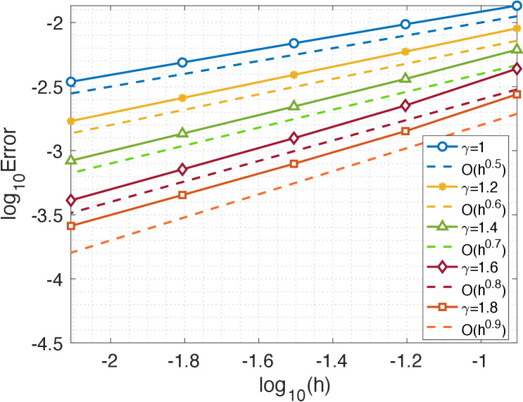
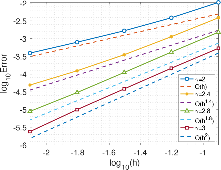
Example 1. (Accuracy test of smooth solutions). We first test the accuracy of the proposed method for the nonlocal BVP (3.19) with and involving a fractional kernel function (2.32) with different values of the parameters .
In the simulation, we use the FEM on uniform meshes, and take the exact solution and (cf. [9, 36]). In Figure 3.2, we plot the numerical errors against various with different parameters . We observe from Figure 3.2 that the convergence order of the piecewise linear FEM on uniform meshes is for fixed horizon , while for fixed horizon , the convergence rate is .
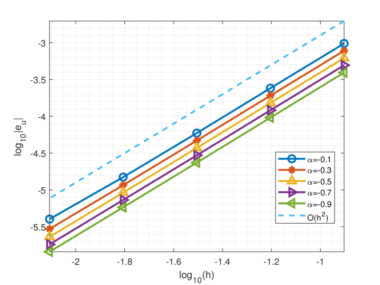
(a) .
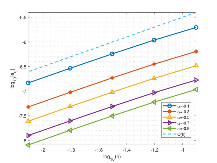
(b) .
Example 2. (Accuracy test of discontinuous solution). Next, we consider the FEM on uniform and graded meshes for the nonlocal BVP (3.19) with and the discontinuous exact solution on given by (cf. [9, 36])
| (3.20) |
In this computation, we take the constant box potential , and choose the following graded meshes
| (3.21) |
where is a suitable grading exponent. Different from (3.3), the above graded meshes clustering near the discontinuous points , which is beneficial for capturing the discontinuous nature of the solution.
In Figure 3.3(a)-(b), we plot the numerical errors of the FEM on uniform meshes with various , which shows that the convergence order is in -norm and in -norm. As a comparison, we plot numerical errors of the FEM on graded meshes with various in Figure 3.3(c)-(d). We observe that, for fixed grading exponent , the -norm errors are roughly of . For fixed grading exponent , i.e., the -norm errors are roughly of . The convergence order of FEM on graded meshes is significantly higher than that of FEM on uniform meshes when there are discontinuities in the solution.
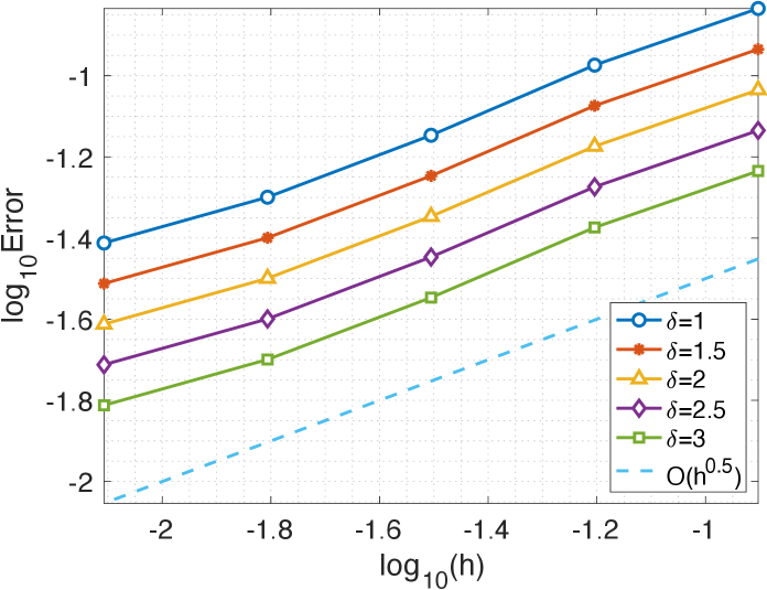
(a) -norm errors.
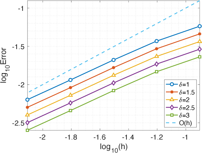
(b) -norm errors.
(c) .
(d) .
(a) uniform meshes.
(b) graded meshes with .
It should be pointed out that no instability has been observed in any of our computations. The piecewise linear FEM we use is not only convergent to the nonlocal constrained value problem with fixed but also convergent to the local differential equation with a fixed ratio between and . Thus, our scheme is an asymptotically compatible scheme [37]. In addition, we find from Figure 3.4 that the numerical solutions of FEM on graded meshes have a better approximation effect and stability than the FEM on uniform meshes at the discontinuity point.
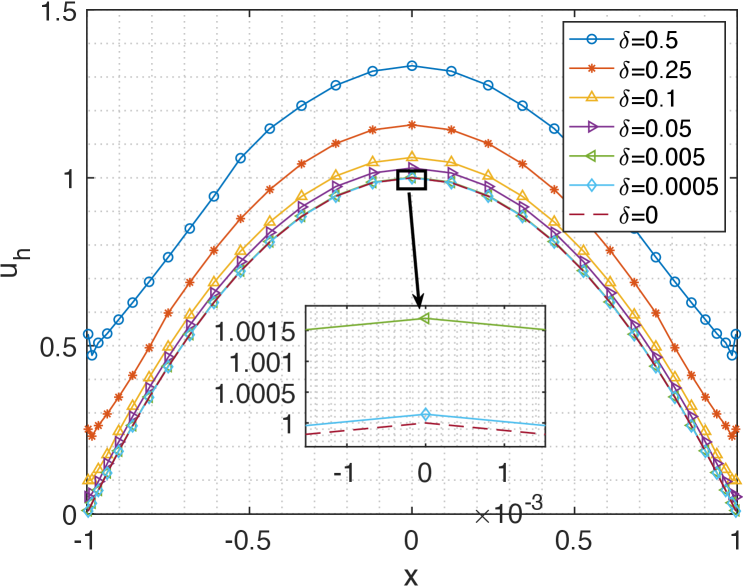
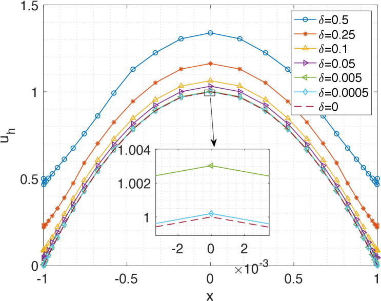
Example 3. (Limiting behaviours). It is interesting to numerically study the local limit (i.e., ) and the nonlocal interactions approach infinite (i.e., ) of the nonlocal BVP (3.19) with . More specifically, we compare solutions of the nonlocal BVP (3.19) with to the ODE (resp. fractional Laplacian equation) equation with special interest in observing behaviors in the local limit (resp. fractional limit ).
Case 1 (local limit): To study the local limit (i.e., ), we adopt the piecewise linear FEM for solving the nonlocal BVP (3.19) with , source function and kernel function (2.32). The exact solution is unknown, but the following ODE
| (3.22) |
has the exact solution .
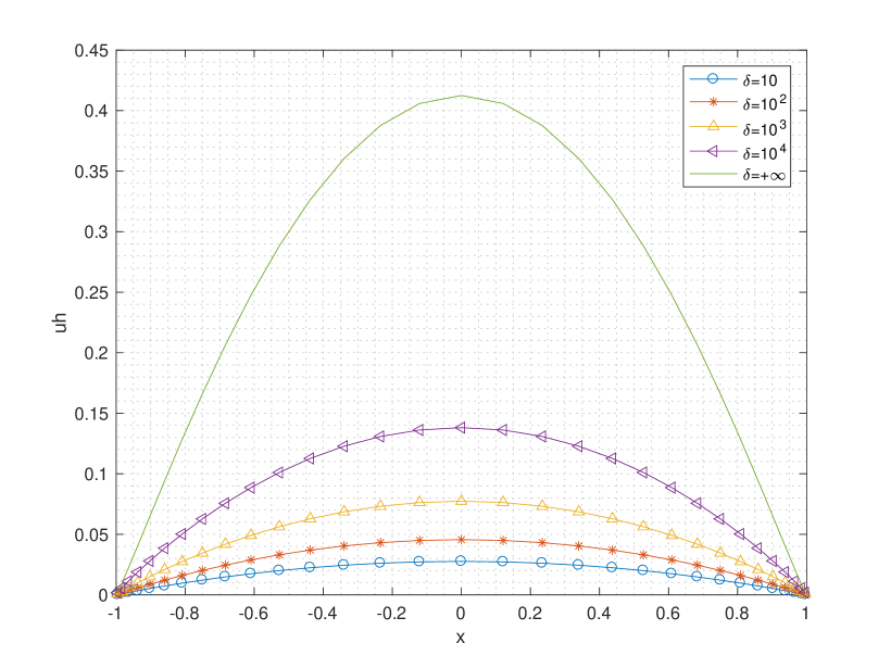
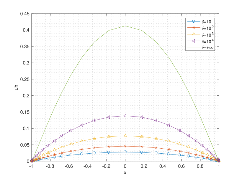
In our computation, we use the graded meshes (3.3). We compare solutions of the nonlocal model to the ODE (3.22) with special interest in observing behaviors in the local limit . Figure 3.10 shows the comparison of numerical solutions for the nonlocal model and the solution of the governing equation given by (3.22) for and , respectively. It can be clearly observed that as , the solution of the nonlocal diffusion model converges to the solution of the local one (3.22).
(a) .
(b) .
(c) .
(d) .
Case 2 (global limit): Now, we turn to the global limit (i.e., ), that is, consider the nonlocal models with the following fractional Laplacian kernel (2.32). It is known that the solution of the nonlocal problem with a fractional Laplacian kernel exhibits singularities near the boundary of . We take and consider a piecewise linear FEM on graded meshes (3.3) for solving the nonlocal BVP (3.19) with and . The exact solution is unknown, but the following fractional Poisson equation
| (3.23) |
where
| (3.24) |
with “p.v.” stands for the principle value. The equation (3.23) admits a exact solution .
As we can see from Figure 3.7, the solution of the nonlocal BVP converges to the solution of the fractional Laplacian equation (3.23) as the nonlocal interactions become infinite, i.e., . Thus the conclusions in [17] are verified numerically.
(a) .
(b) .
3.3.2. Nonlocal BVP with
In this subsection, we will consider the dynamics of nonlocal BVPs (3.19) with .
Example 4. (The dynamics of nonlocal Helmholtz problem). In this example, we will consider the FEM on uniform meshes for the following nonlocal Helmholtz problem
| (3.25) |
where is a given function and is a given constant. Here, we focus on the dynamics of the solution with the following two cases:
Case 1: is continuous function
| (3.26) |
Case 2: is piecewise constant
| (3.27) |
For the convenience of description, we take and the kernel function (2.32), i.e., with fixed .
In Figure 3.8, we depict the profile of the numerical solution for Case 1 on the computation domain with different and . We observe from the top of Figure 3.8 that oscillation in regions with exponential growth and decay in regions with . This observation is consistent with the one described in [39, p.81] for the local model. Moreover, we find from the bottom of Figure 3.8 that as decreases, the oscillation frequency within the oscillatory region amplifies.
In Figure 3.9, we plot the profile of the numerical solution for Case 2 on the computation domain with . It can be seen that the amplitude of the solution is affected by magnitude of the piecewise constant function , that is, the amplitude is larger within the interval , while it is relatively smaller within the interval . We also observe that as decreases, the solution converges to the solution of the local Helmholtz problem, i.e., .
3.3.3. Nonlocal BVP with and is unknown
One fundamental issue in the study of the nonlocal operator is its eigenvalue problem, i.e., (3.19) with and is unknown. Since the spectrum of nonlocal eigenvalue problems depends on the horizon size and the parameters , few analytical results of the eigenvalues or eigenfunctions can be found in the literature, which prompts us to numerical study the nonlocal eigenvalue problem.
Example 5. (Eigenvalue problem) Consider the eigenvalue problem of nonlocal problem with a fractional kernel function (2.32) with different values of the parameters .
| (3.28) |
Using FEM discretization, we can obtain the following standard matrix eigenvalue problem
| (3.29) |
where is the usual FEM mass matrix.
When , is approximating Laplacian operator . As is well known, the Laplacian operator eigenvalue problem with Dirichlet boundary conditions is
| (3.30) |
Its eigenvalues and eigenfunction expressions are
| 2.46740110 | 9.86960440 | 22.20660990 | 39.47841760 | 61.68502751 | ||
|---|---|---|---|---|---|---|
| 2.41759862 | 9.66390067 | 21.71945040 | 38.55295196 | 60.11616374 | ||
| 2.44244850 | 9.76813715 | 21.97209805 | 39.04605489 | 60.97843581 | ||
| 0.4 | 2.45491393 | 9.81923809 | 22.09172241 | 39.27027858 | 61.35199331 | |
| 2.46115693 | 9.84452507 | 22.14980400 | 39.37647857 | 61.52385393 | ||
| 2.46428142 | 9.85710596 | 22.17843509 | 39.42816470 | 61.60622225 | ||
| 2.46584534 | 9.86339180 | 22.19270072 | 39.45381799 | 61.64691606 | ||
| 2.42751075 | 9.70453885 | 21.81459327 | 38.73025554 | 60.41328634 | ||
| 2.44745354 | 9.78841357 | 22.01868176 | 39.13126116 | 61.11637305 | ||
| 0.8 | 2.45742959 | 9.82936677 | 22.11476158 | 39.31185528 | 61.41820329 | |
| 2.46241914 | 9.84959215 | 22.16127618 | 39.39704646 | 61.55634551 | ||
| 2.46491475 | 9.85964614 | 22.18417827 | 39.43844094 | 61.62241698 | ||
| 2.46616355 | 9.86466801 | 22.19558573 | 39.45897877 | 61.65504623 | ||
| 2.43870151 | 9.75058814 | 21.92302394 | 38.93499308 | 60.75718811 | ||
| 2.45296532 | 9.81079299 | 22.07028410 | 39.22610053 | 61.27079425 | ||
| 1.2 | 2.46007728 | 9.84004411 | 22.13911423 | 39.35596052 | 61.48875749 | |
| 2.46362860 | 9.85445490 | 22.17231554 | 39.41690918 | 61.58786858 | ||
| 2.46540354 | 9.86161116 | 22.18863941 | 39.44646660 | 61.63515483 | ||
| 2.46629141 | 9.86518432 | 22.19676697 | 39.46112478 | 61.65849527 | ||
| 2.41843091 | 9.67125122 | 21.75106140 | 38.64553780 | 60.33751981 | ||
| 2.42618623 | 9.70412710 | 21.83198239 | 38.80666199 | 60.62389058 | ||
| 1.6 | 2.43003864 | 9.72000928 | 21.86949303 | 38.87775885 | 60.74384622 | |
| 2.43195879 | 9.72781211 | 21.88751329 | 38.91094086 | 60.79800753 | ||
| 2.43291768 | 9.73168259 | 21.89635993 | 38.92700088 | 60.82378576 | ||
| 2.43339712 | 9.73361430 | 21.90076261 | 38.93496166 | 60.83650391 |
We will test the accuracy of the FEM discretization for eigenvalue of the nonlocal operator (1.2) with a fractional kernel function of the form
with different values of the parameters , which lead to different types of singularities.
| 0 | 1 | ||||||
|---|---|---|---|---|---|---|---|
| 2.4674 | 2.4673 | 2.4668 | 2.4564 | 2.3384 | 1.4074 | ||
| 9.8606 | 9.8694 | 9.8671 | 9.8251 | 9.3226 | 4.4369 | ||
| 2.4674 | 2.4673 | 2.4668 | 2.4558 | 2.3320 | 1.3706 | ||
| 9.8696 | 9.8694 | 9.8670 | 9.8227 | 9.2957 | 4.2549 | ||
| 2.4674 | 2.4673 | 2.4668 | 2.4564 | 2.3384 | 1.4074 | ||
| 9.8696 | 9.8694 | 9.8675 | 9.8274 | 9.4741 | 5.4788 | ||
| 2.4674 | 2.4673 | 2.4668 | 2.4564 | 2.3384 | 1.4074 | ||
| 9.8696 | 9.8694 | 9.8671 | 9.8251 | 9.3226 | 4.4369 |
| 4.98024805e-02 | 2.05703733e-01 | 4.87159503e-01 | 9.26512343e-01 | 1.56886377e+00 | ||
| 2.49526043e-02 | 1.01467251e-01 | 2.34511852e-01 | 4.32362714e-01 | 7.06591693e-01 | ||
| 0.4 | 1.24871709e-02 | 5.03663062e-02 | 1.14887493e-01 | 2.08139023e-01 | 3.33034195e-01 | |
| 6.24417136e-03 | 2.50793326e-02 | 5.68059049e-02 | 1.01939032e-01 | 1.61173579e-01 | ||
| 3.11968427e-03 | 1.24984377e-02 | 2.81748121e-02 | 5.02529059e-02 | 7.88052573e-02 | ||
| 1.55576053e-03 | 6.21259956e-03 | 1.39091786e-02 | 2.45996104e-02 | 3.81114443e-02 | ||
| 3.98903502e-02 | 1.65065555e-01 | 3.92016628e-01 | 7.48162060e-01 | 1.27174116e+00 | ||
| 1.99475595e-02 | 8.11908268e-02 | 1.87928141e-01 | 3.47156447e-01 | 5.68654457e-01 | ||
| 0.8 | 9.97151249e-03 | 4.02376321e-02 | 9.18483274e-02 | 1.66562326e-01 | 2.66824215e-01 | |
| 4.98195687e-03 | 2.00122486e-02 | 4.53337268e-02 | 8.13711451e-02 | 1.28681992e-01 | ||
| 2.48634990e-03 | 9.95825886e-03 | 2.24316343e-02 | 3.99766639e-02 | 6.26105263e-02 | ||
| 1.23755302e-03 | 4.93639234e-03 | 1.10241763e-02 | 1.94388314e-02 | 2.99812714e-02 | ||
| 2.86995852e-02 | 1.19016259e-01 | 2.83585958e-01 | 5.43424529e-01 | 9.27839399e-01 | ||
| 1.44357763e-02 | 5.88114115e-02 | 1.36325797e-01 | 2.52317070e-01 | 4.14233255e-01 | ||
| 1.2 | 7.32381792e-03 | 2.95602930e-02 | 6.74956675e-02 | 1.22457082e-01 | 1.96270021e-01 | |
| 3.77250484e-03 | 1.51494988e-02 | 3.42943660e-02 | 6.15084242e-02 | 9.71589232e-02 | ||
| 1.99755832e-03 | 7.99324535e-03 | 1.79704905e-02 | 3.19510088e-02 | 4.98726797e-02 | ||
| 1.10969274e-03 | 4.42007585e-03 | 9.84292928e-03 | 1.72928194e-02 | 2.65322374e-02 | ||
| 4.89701911e-02 | 1.98353178e-01 | 4.55548502e-01 | 8.32879809e-01 | 1.34750769e+00 | ||
| 4.12148682e-02 | 1.65477295e-01 | 3.74627512e-01 | 6.71755614e-01 | 1.06113693e+00 | ||
| 1.6 | 3.73624593e-02 | 1.49595119e-01 | 3.37116875e-01 | 6.00658756e-01 | 9.41181290e-01 | |
| 3.54423138e-02 | 1.41792288e-01 | 3.19096612e-01 | 5.67476741e-01 | 8.87019975e-01 | ||
| 3.44834248e-02 | 1.37921811e-01 | 3.10249976e-01 | 5.51416724e-01 | 8.61241744e-01 | ||
| 3.40039801e-02 | 1.35990099e-01 | 3.05847296e-01 | 5.43455943e-01 | 8.48523597e-01 |
| 0.9970 | 1.0196 | 1.0547 | 1.0996 | 1.1508 | ||
| 0.9987 | 1.0105 | 1.0294 | 1.0547 | 1.0852 | ||
| 0.4 | 0.9999 | 1.0060 | 1.0161 | 1.0298 | 1.0471 | |
| 1.0011 | 1.0048 | 1.0116 | 1.0204 | 1.0323 | ||
| 1.0038 | 1.0085 | 1.0184 | 1.0306 | 1.0481 | ||
| 0.9998 | 1.0237 | 1.0607 | 1.1078 | 1.1612 | ||
| 1.0003 | 1.0128 | 1.0329 | 1.0595 | 1.0917 | ||
| 0.8 | 1.0011 | 1.0077 | 1.0187 | 1.0335 | 1.0521 | |
| 1.0027 | 1.0069 | 1.0151 | 1.0254 | 1.0393 | ||
| 1.0065 | 1.0124 | 1.0249 | 1.0402 | 1.0623 | ||
| 0.9914 | 1.0170 | 1.0567 | 1.1068 | 1.1634 | ||
| 0.9790 | 0.9924 | 1.0142 | 1.0430 | 1.0776 | ||
| 1.2 | 0.9571 | 0.9644 | 0.9768 | 0.9934 | 1.0144 | |
| 0.9173 | 0.9224 | 0.9323 | 0.9449 | 0.9621 | ||
| 0.8481 | 0.8547 | 0.8685 | 0.8857 | 0.9105 | ||
| 0.2487 | 0.2614 | 0.2821 | 0.3102 | 0.3447 | ||
| 0.1416 | 0.1456 | 0.1522 | 0.1614 | 0.1731 | ||
| 1.6 | 0.0761 | 0.0773 | 0.0793 | 0.0820 | 0.0855 | |
| 0.0396 | 0.0399 | 0.0406 | 0.0414 | 0.0425 | ||
| 0.0202 | 0.0203 | 0.0206 | 0.0210 | 0.0215 |
Tables 3.1 provide numerical eigenvalues of FEM on graded meshes. A large amount of experimental results can observe three phenomena: 1) When , the eigenvalues of nonlocal operator tend to the corresponding eigenvalues of local Laplacian operator (3.30); 2) The eigenvalues of local Laplacian operator (3.30) are the upper bound of the corresponding eigenvalues of nonlocal operator; 3) The smaller the horizon parameter , the larger the eigenvalues of nonlocal operator.
(1).
(2).
(3).
(4).
(1).
(2).
(3).
(4).
As shown in the Figure 3.10-3.11, whether using a uniform grid or a non-uniform grid, it becomes evident that as , the eigenvalues and eigenfunctions of nonlocal operator (1.2) all convergence to those of the classical Laplace operator.
(1).
(2).
(3).
(1).
(2).
(3).
According to the Figure (3.12), we observe that as increases, the error between the numerical solution of the eigenvalue and the exact solution becomes progressively larger. However, the calculated numerical solutions are consistently smaller than the exact solutions, allowing us to establish a lower bound for the eigenvalue obtained through this method. We can get the following conclusions (???):
| 4.03e-02 | 1.68e-01 | ||||
| 1.65e-02 | 1.288 | 6.76e-02 | 1.313 | ||
| 0.25 | 7.13e-03 | 1.210 | 2.85e-02 | 1.244 | |
| 3.29e-03 | 1.118 | 1.24e-02 | 1.201 | ||
| 1.51e-03 | 1.125 | 4.92e-03 | 1.336 | ||
| 3.17e-02 | 1.32e-01 | ||||
| 1.31e-02 | 1.280 | 5.34e-02 | 1.310 | ||
| 0.75 | 5.36e-03 | 1.285 | 2.13e-02 | 1.330 | |
| 2.07e-03 | 1.370 | 7.46e-03 | 1.510 | ||
| 5.33e-04 | 1.960 | 9.74e-04 | 2.937 | ||
| 3.65e-02 | 1.50e-01 | ||||
| 2.40e-02 | 0.606 | 9.66e-02 | 0.634 | ||
| 1.25 | 1.85e-02 | 0.375 | 7.36e-02 | 0.392 | |
| 1.61e-02 | 0.206 | 6.33e-02 | 0.219 | ||
| 1.49e-02 | 0.109 | 5.83e-02 | 0.117 | ||
| 5.51e-01 | 2.21e+00 | ||||
| 5.46e-01 | - | 2.19e+00 | - | ||
| 1.75 | 5.43e-01 | - | 2.17e+00 | - | |
| 5.43e-01 | - | 2.17e+00 | - | ||
| 5.42e-01 | - | 2.17e+00 | - |
3.4. Time-dependent problem
Consider the following nonlocal Allen-Cahn equation:
| (3.31) |
where is the initial data, is given function on satisfies with . In the above, is the nonlocal operator (1.2) and is a constant.
Let be a positive integer and be a time step size. We can get the time grid and use to approximate , . Using backward Euler method to approximate , we can get
Here, we employ the fully discrete scheme with the semi-implicit scheme in time and FEM discretization in space for solving the problem (3.31): find , such that
| (3.32) |
Then, it is easy to obtain the matrix form of (3.32) as follows:
| (3.33) |
where is the usual (tridiagonal) FEM mass matrix, the stiffness matrix is defined in (2.13), and is defined as
In this example, we adopt the proposed fully discrete scheme (3.32) to simulate the phase evolution behavior and energy dissipation. We take , , the initial date , and take the fractional kernel function of the form (2.32).
| 2.45e-03 | 2.55e-03 | ||||
| 1.23e-03 | 0.995 | 1.28e-03 | 0.993 | ||
| 0.25 | 6.16e-04 | 0.998 | 6.43e-04 | 0.997 | |
| 3.08e-04 | 0.999 | 3.22e-04 | 0.999 | ||
| 1.54e-04 | 0.999 | 1.61e-04 | 0.999 | ||
| 2.45e-03 | 2.54e-03 | ||||
| 1.23e-03 | 0.995 | 1.27e-03 | 0.994 | ||
| 0.75 | 6.15e-04 | 0.998 | 6.38e-04 | 0.997 | |
| 3.08e-04 | 0.998 | 3.20e-04 | 0.999 | ||
| 1.54e-04 | 0.999 | 1.60e-04 | 0.999 | ||
| 2.45e-03 | 2.52e-03 | ||||
| 1.23e-03 | 0.995 | 1.26e-03 | 0.994 | ||
| 1.25 | 6.16e-04 | 0.998 | 6.33e-04 | 0.997 | |
| 3.08e-04 | 0.999 | 3.17e-04 | 0.999 | ||
| 1.54e-04 | 0.999 | 1.59e-04 | 0.999 | ||
| 2.57e-03 | 2.60e-03 | ||||
| 1.29e-03 | 0.995 | 1.30e-03 | 0.994 | ||
| 1.75 | 6.45e-04 | 0.997 | 6.53e-04 | 0.997 | |
| 3.23e-04 | 0.999 | 3.27e-04 | 0.999 | ||
| 1.61e-04 | 0.999 | 1.63e-04 | 0.999 | ||
| 9.57e-03 | 0.145 | 9.90e-03 | 0.154 | ||||
| 2.38e-03 | 2.006 | 0.409 | 2.42e-03 | 2.034 | 0.359 | ||
| 0.25 | 6.02e-04 | 1.985 | 1.869 | 6.05e-04 | 1.999 | 1.925 | |
| 1.51e-04 | 1.998 | 8.405 | 1.51e-04 | 2.000 | 8.535 | ||
| 3.77e-05 | 1.999 | 47.98 | 3.78e-05 | 2.000 | 49.09 | ||
| 9.56e-03 | 0.142 | 9.87e-03 | 0.142 | ||||
| 2.38e-03 | 2.006 | 0.360 | 2.41e-03 | 2.032 | 0.380 | ||
| 0.75 | 6.01e-04 | 1.986 | 1.974 | 6.04e-04 | 1.997 | 1.884 | |
| 1.50e-04 | 1.997 | 8.415 | 1.51e-04 | 2.000 | 8.461 | ||
| 3.77e-05 | 1.998 | 47.17 | 3.78e-05 | 1.999 | 47.11 | ||
| 9.55e-03 | 0.142 | 9.81e-03 | 0.140 | ||||
| 2.38e-03 | 2.006 | 0.380 | 2.40e-03 | 2.029 | 0.350 | ||
| 1.25 | 5.99e-04 | 1.988 | 1.884 | 6.04e-04 | 1.993 | 1.952 | |
| 1.50e-04 | 1.996 | 8.461 | 1.51e-04 | 2.000 | 8.400 | ||
| 3.76e-05 | 1.997 | 47.11 | 3.78e-05 | 1.999 | 47.10 | ||
| 9.64e-03 | 0.200 | 9.78e-03 | 0.211 | ||||
| 2.38e-03 | 2.017 | 0.438 | 2.40e-03 | 2.027 | 0.544 | ||
| 1.75 | 6.00e-04 | 1.989 | 2.565 | 6.04e-04 | 1.991 | 2.262 | |
| 1.51e-04 | 1.997 | 12.73 | 1.51e-04 | 1.999 | 13.02 | ||
| 3.76e-05 | 1.997 | 63.23 | 3.79e-05 | 1.997 | 56.96 | ||
(a) .
(b) .
(c) .
(d) .
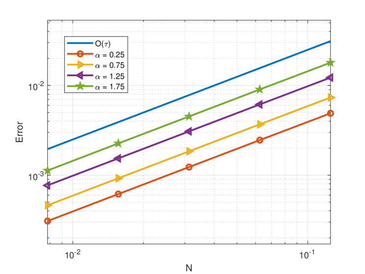
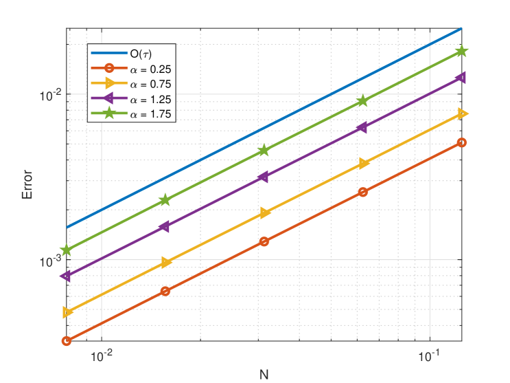
In Figure 3.13, we plot the numerical errors and the corresponding convergence rates of the proposed method max errors for different and . As we can see the temporal convergence rate is , and the space convergence rate is . Moreover, we display the waveform of the numerical solution at the different and time, see Figures 3.14. The dates indicate that the affects the propagation velocity of the solitary wave. For a smaller , the propagation of the soliton becomes slower, thus indicating the presence of quantum sub-diffusion. Finally, we plot the evolution of maximum value at various times with different and in Figure 3.15, which shows that the maximum principle is preserved numerically. We observe from Figure 3.15 (d) that the maximum value of the steady state is increased as increases.
(a) .
(b) .
(c) .
(d) .
we consider the following two-grid system based on finite element method, which includes the space coarse mesh in and the space fine mesh in . Now, we use the two-grid method and give its fully discrete scheme.
Step 1: We choose the coarse meshes which the step size is in , then we have
If , then we can building the fully implicit finite element scheme of the problem (3.31) such follows:
| (3.34) |
Step 2: We choose the fine meshes which the step size is . Then we have
In the fine meshes, the nonlinear term is calculated by , then we can building the semi-implicit finite element scheme as follows:
| (3.35) |
Finally, we can give the next matrix equations for completing (3.34)-(3.35) which are:
Step 1: The matrix equation of (3.34) is
| (3.36) |
where is the usual (tridiagonal) FEM stiffness matrix which step size is on uniform meshes, the stiffness matrix is defined in the above. are defined as follows:
In this step, we use (3.37) to complete (3.36). It is
| (3.37) |
where is the usual (tri-diagonal) FEM stiffness matrix in coarse meshes, the stiffness matrix is defined in the above. And are defined as follows:
where is the iteration steps ().
Step 2: Based on the solutions in Step 1 and the basis functions of the finite element method in the coarse meshes, we have
| (3.38) |
Step 3: Utilizing the solutions obtained from Step 2, the matrix equation of (3.35) is
| (3.39) |
where is the usual (tri-diagonal) FEM stiffness matrix in the fine meshes, the stiffness matrix is defined in the above. is defined as follows:
| Max error | Rate | CPU(s) | Max error | Rate | CPU(s) | |||
|---|---|---|---|---|---|---|---|---|
| 6.17e-01 | 0.269 | 6.25e-01 | 2.083 | |||||
| 3.04e-02 | 2.171 | 1.312 | 3.08e-02 | 2.171 | 10.42 | |||
| 0.25 | 1.22e-03 | 2.320 | 7.847 | 1.22e-03 | 2.328 | 69.42 | ||
| 5.96e-05 | 2.176 | 73.88 | 5.96e-05 | 2.179 | 664.88 | |||
| 3.73e-06 | 2.000 | 1363.3 | 3.73e-06 | 2.000 | 12720.3 | |||
4. Concluding remarks and discussions
Different from the implementation of FEM in the physical space, we evaluated the nonlocal stiffness matrix of piecewise linear FEM for the nonlocal operator in the Fourier-transformed domain, and derived the explicit integral form of the entries on non-uniform meshes. This allowed us to adopt the different meshes for different situations, and enabled us to resort to the Gauss quadrature for one dimension integral accurately. Plenty of numerical examples for solving the nonlocal models are presented to demonstrate the accuracy and efficiency of the proposed method.
The current study is largely based on a simple one-dimensional linear model for the sake of offering insight without being impeded by tedious calculations. More careful studies on the stability and convergence analysis of piecewise linear FEM on non-uniform meshes, and one may extend the study to two-dimensional rectangular elements, but it is more involved, which we shall report in a future work.
Declarations
Conflict of interest The authors declare that they have no conflict of interest.
Appendix A Evaluation of the distance matrix
For , tedious but straightforward calculations show that in (2.14) are
-
(i)
For
(A.1) -
(ii)
For
(A.2) -
(iii)
For
(A.3) -
(iv)
For
(A.4) -
(v)
For
(A.5) -
(vi)
For
(A.6) -
(vii)
For
(A.7)
References
- [1] M. Abramovitz and I. A. Stegun, Handbook of Mathematical Functions, Dover, New York, 1972.
- [2] G. Acosta and J. P. Borthagaray, A fractional Laplace equation: regularity of solutions and finite element approximations, SIAM J. Numer. Anal., 55(2017)472–495.
- [3] M. Ainsworth and C. Glusa, Aspects of an adaptive finite element method for the fractional Laplacian: a priori and a posteriori error estimates, efficient implementation and multigrid solver, Comput. Methods Appl. Mech. Engrg., 327(2017)4-35.
- [4] B. Aksoylu and Z. Unlu, Conditioning analysis of nonlocal integral operator in fractional Sobolev spaces, SIAM J. Numer. Anal., 52(2014)653-677.
- [5] E. Askari, F. Bobaru, R. B. Lehoucq, M. L. Parks, S. A. Silling and O. Weckner, Peridynamics for multiscale materials modeling, Journal of Physics: Conference Series, 2008.
- [6] E. Aulisa, G. Capodaglio, A. Chierici, M. D’Elia, Marta, Efficient quadrature rules for finite element discretizations of nonlocal equations, Numer. Methods Partial Differential Equations, 38(2022)1767–1793.
- [7] A. Bonito, J. P. Borthagaray, R. H. Nochetto, E. Otárola and A. J. Salgado, Numerical methods for fractional diffusion, Comput. Vis. Sci., 19 (2018)19-46.
- [8] R. Cao, M. Chen, Y. Qi, J. Shi, X. Yin, Analysis of (shifted) piecewise quadratic polynomial collocation for nonlocal diffusion model, Appl. Numer. Math. 185(2023)120–140.
- [9] X. Chen, M. Gunzburger, Continuous and discontinuous finite element methods for a peridynamics model of mechanics, Comput. Methods Appl. Mech. Engrg., 200(2011)1237-1250.
- [10] H. Chen, C. Sheng, and L.-L Wang, On explicit form of the FEM stiffness matrix for the integral fractional Laplacian on non-uniform meshes, Appl. Math. Lett., 113(2021)106864.
- [11] I. S. Gradshteyn and I. M. Ryzhik, Table of Integrals, Series and Products, Seven Edition, Elsevier, 2007.
- [12] Q. Du, M. Gunzburger, R. Lehoucq and K. Zhou, Analysis and approximation of nonlocal diffusion problems with volume constraints, SIAM Review, 54(2012)667-696.
- [13] Q. Du, M. Gunzburger, R. Lehoucq and K. Zhou, A posteriori error analysis of finite element method for linear nonlocal diffusion and peridynamic models, Math. Comp., 82(2013)1889-1922.
- [14] Q. Du, Nonlocal Modeling, Analysis, and Computation, Society for Industrial and Applied Mathematics, Philadelphia, 2019.
- [15] Q. Du, X. Tian and Z. Zhou Nonlocal diffusion models with consistent local and fractional limits, A³N²M: Approximation, Applications, and Analysis of Nonlocal, Nonlinear Models, The IMA Volumes in Mathematics and its Applications, Springer, Cham. 165(2023)175–213.
- [16] S. Duo, H. van Wyk and Y. Zhang, A novel and accurate finite difference method for the fractional Laplacian and the fractional poisson problem, J. Comput. Phys., 355(2018)233-252.
- [17] M. D’Elia, M. Gunzburger, The fractional Laplacian operator on bounded domains as a special case of the nonlocal diffusion operator, Comput. Math. Appl., 66(2013)1245– 1260.
- [18] M. D’Elia, Q. Du, C. Glusa, M. Gunzburger, X. Tian, and Z. Zhou, Numerical methods for nonlocal and fractional models, Acta Numer., 29(2020)1-124.
- [19] E. Di Nezza, G. Palatucci, and E. Valdinoci, Hitchhiker’s guide to the fractional Sobolev spaces, Bull. Sci. Math. 136(2012)521–573.
- [20] I. Fried, Condition of finite element matrices generated from nonuniform meshes, AIAA J. 10(1972)219-221.
- [21] Q. Guan, M. Gunzburger, X. Zhang, Collocation method for one dimensional nonlocal diffusion equations, Numer. Methods Partial Differential Equations, 38(2022)1618–1635.
- [22] Z. Hao, Z. Zhang and R. Du, Fractional centered difference scheme for high-dimensional integral fractional Laplacian, J. Comput. Phys., 424(2021)109851.
- [23] Y. Huang, A. Oberman, Numerical methods for the fractional Laplacian: a finite difference-quadrature approach, SIAM J. Numer. Anal., 52(2014)3056-3084.
- [24] M. Klar, G. Capodaglio, M. D’Elia, C. Glusa, M. Gunzburger, Max, and C. Vollmann, A scalable domain decomposition method for FEM discretizations of nonlocal equations of integrable and fractional type, Comput. Math. Appl. 151(2023)434-448.
- [25] Y. Leng, X. Tian, N. Trask, J. T. Foster, Asymptotically compatible reproducing kernel collocation and meshfree integration for nonlocal diffusion, SIAM J. Numer. Anal. 59(2021)88–118.
- [26] H. Li, R. Liu and L.-L. Wang, Efficient Hermite spectral-Galerkin methods for nonlocal diffusion equations in unbounded domains, Numer. Math. Theo. Meth. Appl., 15 (2022)1009-1040.
- [27] A. Lischke, G. Pang, M. Gulian, and et al., What is the fractional Laplacian? A comparative review with new results, J. Comput. Phys., 404(2020)109009.
- [28] Z. Liu, A. Cheng and H. Wang, An hp-Galerkin method with fast solution for linear peridynamic models in one dimension, Comp. Math. Appl., 73(2017)1546-1565.
- [29] H. Liu, C. Sheng, L.-L. Wang, and H. Yuan, On diagonal dominance of FEM stiffness matrix of fractional Laplacian and maximum principle preserving schemes for fractional Allen-Cahn equation, J. Sci. Comput., 86(2021)19.
- [30] J. Lu, Y. Nie, A reduced-order fast reproducing kernel collocation method for nonlocal models with inhomogeneous volume constraints, Comput. Math. Appl. 121(2022)52–61.
- [31] Z. Mao, J. Shen, Hermite spectral methods for fractional PDEs in unbounded domains, SIAM J. Sci. Comput., 39(2017)A1928-A1950.
- [32] H. Wang, H. Tian, A fast and faithful collocation method with efficient matrix assembly for a two-dimensional nonlocal diffusion model, Comput. Methods Appl. Mech. Engrg., 273(2014)19-36.
- [33] C. Sheng, J. Shen, T. Tang, L. L. Wang and H. Yuan, Fast Fourier-like mapped Chebyshev spectral-Galerkin methods for PDEs with integral fractional Laplacian in unbounded domains, SIAM J. Numer. Anal., 58(2020)2435-2464.
- [34] C. Sheng, L. L. Wang, H. Chen and H. Li, Fast implementation of FEM for integral fractional Laplacian on rectangular meshes, Commun. Comput. Phys., 35(2024).
- [35] T. Tang, L.L. Wang, H. Yuan and T. Zhou, Rational spectral methods for PDEs involving fractional Laplacian in unbounded domains, SIAM J. Sci. Comput., 42 (2020)A585-A611.
- [36] X. Tian and Q. Du, Analysis and comparison of different approximations to nonlocal diffusion and linear peridynamic equations, SIAM J. Numer. Anal., 51(2013)3458-3482.
- [37] X. Tian and Q. Du, Asymptotically compatible schemes for robust discretization of nonlocal models and their local limits, SIAM J. Numer. Anal., 52(2014)1641-1665.
- [38] X. Tian, Q. Du and M. Gunzburger, Asymptotically compatible schemes for the approximation of fractional Laplacian and related nonlocal diffusion problems on bounded domains, Adv. Comput. Math., 42(2016)1363–1380.
- [39] L. Trefethen, Á. Birkisson, and T. A. Driscoll, Exploring ODEs. Society for Industrial and Applied Mathematics, Philadelphia, PA, 2018.
- [40] Q. Ye and X. Tian, Monotone meshfree methods for linear elliptic equations in non-divergence form via nonlocal relaxation, J. Sci. Comput. 96 (2023)33.
- [41] C. Zheng, J. Hu, Q. Du, and J. Zhang, Numerical solution of the nonlocal diffusion equation on the real line, SIAM J. Sci. Comput., 39(2017)A1951-A1968.
- [42] K. Zhou and Q. Du, Mathematical and numerical analysis of linear peridynamic models with nonlocal boundary conditions, SIAM J. Numer. Anal., 48(2010)1759-1780.