Field Sources for Generalized Ellis-Bronnikov Wormhole

As previously mentioned, the EB wormhole metric is a solution to Einstein’s field equation, where a massless scalar field with negative energy acts as the source of curvature. The metric is typically expressed as

$$ds^{2}=-dt^{2}+\frac{dr^{2}}{\left(1-\frac{b(r)}{r}\right)}+r^{2}d\Omega^{2},$$

(5)

witch corresponds to the wormhole metric introduced by Morrison and Thorne Morris1988WormholesIS , with a trivial redshift function. Here, $b(r)$ is the shape function that governs the behavior of the wormhole.

The non-zero components of the Einstein tensor for the metric (5) are

$$G^{t}_{t}=-\frac{b^{\prime}(r)}{r^{2}},$$

(6)

$$G^{r}_{r}=-\frac{b(r)}{r^{3}},$$

(7)

$$G^{\theta}_{\theta}=G^{\varphi}_{\varphi}=\frac{b(r)-rb^{\prime}(r)}{2r^{3}}.$$

(8)

For the EB wormhole, the shape function takes on a particular form:

$$b(r)=\frac{b_{0}^{2}}{r}$$

(9)

where $b_{0}$ is the radius of the wormhole’s throat. The geometry of the solution describes a ”tunnel” that connects two distinct regions of spacetime through the throat. This solution is one of the simplest types of wormhole solutions.

Through a change of coordinates given by

$$dl^{2}=\frac{dr^{2}}{\left(1-\frac{b_{0}^{2}}{r^{2}}\right)}$$

(10)

it is possible to express the metric as (1).

We can also express the GEB metric in terms of $r$, where the metric takes the form given in (5), where now

$$b(r)=r-r^{3-2m}(r^{m}-b_{0}^{m})^{2-\frac{2}{m}}.$$

(11)

Setting $t=cte$ and considering the spherical symmetry of the wormhole geometry, we can, without loss of generality, choose $\theta=\pi/2$ in (4). This yields the 2D geometry described by

$$ds^{2}_{2D}=dl^{2}+(l^{m}+b_{0}^{m})^{2/m}d\varphi^{2}.$$

(12)

We can embed this curved 2D geometry into a 3D Euclidean geometry given by the line element

$$d\sigma^{2}_{3D}=d\rho^{2}+\rho^{2}d\varphi^{2}+dz^{2}=\left[\left(\frac{d\rho(l)}{dl}\right)^{2}+\left(\frac{dz(l)}{dl}\right)^{2}\right]dl^{2}+\rho^{2}d\varphi^{2},$$

(13)

where we identify

$$\rho(l)=(b_{0}^{m}+l^{m})^{1/m},$$

(14)

$$\frac{dz}{dl}=(1-l^{-2+2m}(b_{0}^{m}+l^{m})^{-2+2/m})^{1/2}$$

(15)

Numerically integrating the equation (15) with $b_{0}=1$ for different values of $m$ allows us to create the immersion diagram for this GEB wormhole, as represented in Fig. 1, where we can observe the classical geometry of a catenoid for $m=2$. For $m>2$, the geometry of the neck of the GEB wormhole increasingly tends to become cylindrical.

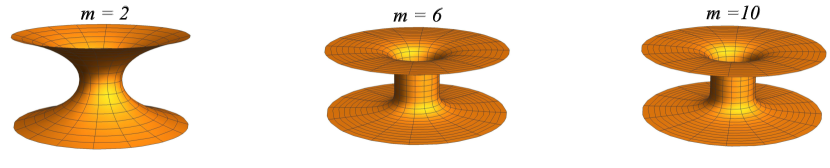
Although the energy conditions continue to be violated for this class of wormholes Kar:1995jz , the fact that the geometry of the wormhole flattens more rapidly with the increase of $m$ has as one of its consequences the occurrence of resonance in the transmission of massless waves in this geometry, which can be used as a means of obtaining information about the size of the wormhole’s throat Kar:1995jz , and others studies suggest that this family of wormholes can be used as a template for exploring the gravitational wave physics of exotic compact objects DuttaRoy:2019hij , and may also serve as a potential black hole mimicker Roy:2021jjg , pending confirmation of stability under all types of perturbations, with initial comparisons of their ringdown characteristics to black holes supporting this idea. Furthermore, it is important to emphasize that this family of solutions has been studied in other contexts beyond GR, such as in braneworld models Sharma:2022tiv ; Sharma:2022dbx ; Sharma:2021kqb , modified gravity models Godani:2023jhq ; Muniz:2022aal ; Nilton:2022hrp , and even in condensed matter contexts deSouza:2022ioq .

The accretion process of a fluid onto a black hole is already well documented in the literatureMach:2013gia ; Yang:2015sfa ; Bahamonde:2015uwa ; Ahmed:2016cuy ; Azreg-Ainou:2018wjx ; Neves:2019ywx ; Panotopoulos:2021ezt . However, the study of accretion in wormhole geometries remains a relatively unexplored topic Rueda:2023val ; Combi:2024ehi , making the analysis of dust accretion (a pressureless fluid) particularly interesting to investigate in the wormhole geometry considered here.

The energy-momentum tensor for dust is given by

$$T_{\mu\nu}=\rho u_{\mu}u_{\nu},$$

(16)

where $\rho$ is the energy density and $u$ is the four-velocity of the fluid, defined as

$$u^{\mu}\equiv\frac{dx^{\mu}}{d\tau}=(u^{t},u^{r},0,0)$$

(17)

with proper time $\tau$, where from now on we will denote the radial velocity as $u^{r}\equiv u$. Here we will assume radial accretion, so that we are assuming $u^{\theta}=u^{\varphi}=0$. From the normalization condition $u^{\mu}u_{\mu}=-1$, we can relate $u^{t}$ to $u^{r}$ as

$$u^{t}=\sqrt{\frac{u^{2}}{\left(1-\frac{b_{0}^{m}}{r^{m}}\right)^{2-2/m}}+1}.$$

(18)

On the other hand, the conservation equation of the energy-momentum tensor, $\nabla_{\mu}T^{\mu\nu}=0$, implies

$$\frac{\rho ur^{2}}{\left(1-\frac{b_{0}^{m}}{r^{m}}\right)^{2-2/m}}\sqrt{u^{2}+\left(1-\frac{b_{0}^{m}}{r^{m}}\right)^{2-2/m}}=C_{1},$$

(19)

where $C_{1}$ is an integration constant. Next, we will consider the equation for the conservation of mass flux, given by $\nabla_{\mu}J^{\mu}$, where $J^{\mu}=u_{\nu}T^{\mu\nu}$, which leads us to the expression

$$\frac{\rho ur^{2}}{\sqrt{\left(1-\frac{b_{0}^{m}}{r^{m}}\right)^{2-2/m}}}=C_{2},$$

(20)

where $C_{2}$ is another integration constant. By dividing the equations (19) and (20), we obtain

$$\sqrt{\frac{u^{2}}{\left(1-\frac{b_{0}^{m}}{r^{m}}\right)^{2-2/m}}+1}=\frac{C_{1}}{C_{2}}\equiv C_{4}.$$

(21)

With this, we can finally obtain expressions for $u$ and $\rho$

	$\displaystyle u$	$\displaystyle=$	$\displaystyle\pm\sqrt{\left(1-\frac{b_{0}^{m}}{r^{m}}\right)^{2-2/m}({C^{(m)}_{4}}^{2}-1)},$		(22)
	$\displaystyle\rho$	$\displaystyle=$	$\displaystyle\frac{C^{(m)}_{2}}{\sqrt{{C^{(m)}_{4}}^{2}-1}}\frac{1}{r^{2}},$		(23)

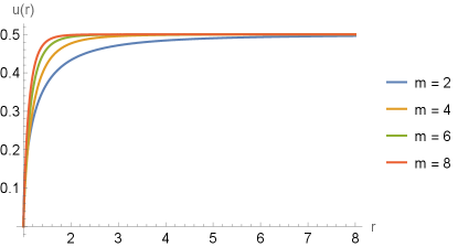
where the signal $\pm$ indicates ingoing (outgoing) fluid and the constants are determined by the initial conditions at the bondary $r_{i}=500b_{0}$. They are indexed by $m$ because, for a given initial condition $(u_{i},\rho_{i})$, ${C^{(m)}_{4}}$ and $C^{(m)}_{2}$ will depend on the value of $m$. We will consider the following initial conditions for the radial velocity and energy density: $u_{i}=0.5$ and $\rho_{i}=0.001$. In Fig. 2, we present the plot of the radial velocity $u$ as functions of the coordinate $r$, for different values of $m$. By analyzing the plot, we observe that the radial velocity decreases as the particle approaches the throat of the wormhole, in agreement with the results reported in Rueda:2023val . This behavior contrasts with the typical case of black holes Bahamonde:2015uwa , where the radial velocity increases as $r$ decreases. However, an important feature in our case is that, as the parameter $m$ increases, the radial velocity decreases more gradually with decreasing $r$, until it eventually drops abruptly to zero near the throat for sufficiently large values of $m$.

By analyzing the expression (23) for the energy density, we observe that its behavior does not vary significantly with the parameter $m$. The density falls off as $1/r^{2}$ and reaches its maximum at the throat, suggesting that the highest concentration of matter is localized around this region, as expected. Another important point to highlight is that the energy density remains regular throughout the entire spacetime, in contrast to the typical behavior in black holes Rueda:2023val , where singularities usually arise.

To conclude our analysis, we examine the rate of change of the mass $\dot{M}$ of the dust traversing the GEB wormhole, which corresponds to the flux integral given by Debnath:2015hea

$\displaystyle\dot{M}=\int T_{0}^{1}\sqrt{-g}d\theta d\varphi,$

(24)

which in our case leads to

$\displaystyle\dot{M}=4\pi C^{(m)}_{2}\left(1-\frac{b_{0}^{m}}{r^{m}}\right)^{2-2/m}\sqrt{u^{2}\left(1-\frac{b_{0}^{m}}{r^{m}}\right)^{2-2/m}+1}.$

(25)

It is worth highlighting, as pointed out in Rueda:2023val , that contrary to what occurs in black hole scenarios, matter is not accumulated in this case, but should be interpreted as the matter traversing the throat of the wormhole. In Fig. 3 we have the plot of $\dot{M}$ for different values of $m$.

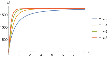
Observing the plot above, we see that the rate of mass change decreases as we approach the wormhole throat, following the behavior of the radial velocity, which also decreases near the throat.

In the framework of GR, in the next section, we calculate the fields that serve as sources for this geometry.

Let’s consider an action of the form

$$S=\int\sqrt{-g}d^{4}x\left(R-2\epsilon g^{\mu\nu}\partial_{\mu}\phi\partial_{\nu}\phi+2V(\phi)+\mathcal{L(F)}\right),$$

(26)

where $\phi$ is a scalar field, $V(\phi)$ is the potential associated to the scalar field and $\mathcal{L(F)}$ is the Lagrangian density of the nonlinear electromagnetic field with $\mathcal{F}=F^{\mu\nu}F_{\mu\nu}$, where $F_{\mu\nu}$ is the electromagnetic field tensor. Furthermore, $\epsilon=-1$ for a phantom scalar field and $\epsilon=+1$ for a canonical scalar field.

Varying the action with respect to the metric $g^{\mu\nu}$ yields Einstein’s equation

$$G_{\mu\nu}=R_{\mu\nu}-\frac{1}{2}Rg_{\mu\nu}=T_{\mu\nu}[\phi]+T_{\mu\nu}[\mathcal{F}],$$

(27)

where $T_{\mu\nu}[\phi]$ e $T_{\mu\nu}[\mathcal{F}]$ are, respectively, the energy-momentum tensor associated with the scalar field and the nonlinear electromagnetic field, given by

$$T_{\mu\nu}[\phi]=2\epsilon\partial_{\mu}\phi\partial_{\nu}\phi-g_{\mu\nu}\left(\epsilon g^{\lambda\rho}\partial_{\lambda}\phi\partial_{\rho}\phi-V(\phi)\right),$$

(28)

$$T_{\mu\nu}[\mathcal{F}]=g_{\mu\nu}\frac{\mathcal{L(F)}}{2}-2\mathcal{L_{F}}F^{\alpha}_{\mu}F_{\nu\alpha},$$

(29)

where$\mathcal{L_{F}}=d\mathcal{L}/d\mathcal{F}$. Varying the action with respect to the scalar field $\phi$ and the electromagnetic field $F_{\mu\nu}$ we obtain the equations for the fields

$$2\epsilon\nabla_{\mu}\nabla^{\mu}\phi=-\frac{dV(\phi)}{d\phi},$$

(30)

$$\nabla_{\mu}(\mathcal{L_{F}}F^{\mu\nu})=0.$$

(31)

In addition to assuming a radial scalar field $\phi=\phi(r)$, we also assume here only the existence of a radial magnetic field, i.e., that the only non-zero components of the electromagnetic tensor $F_{\mu\nu}$ are given by $F_{\theta\varphi}=-F_{\varphi\theta}=q_{m}\sin\theta$, where $q_{m}$ is the charge of the magnetic monopole. With this, we have that the invariant $\mathcal{F}$ is given by

$$\mathcal{F}=\frac{2q_{m}^{2}}{r^{4}}.$$

(32)

With the metric given in 5, the components of the energy momentum tensors for $\phi$ and $F_{\mu\nu}$ take the form

$$T_{\mu}^{\nu}[\phi]=V(\phi)\delta_{\mu}^{\nu}-\epsilon\left(1-\frac{b(r)}{r}\right)\phi^{\prime}(r)^{2}\text{diag(1,-1 ,1 ,1)},$$

(33)

$$T_{\mu}^{\nu}[\mathcal{F}]=\frac{1}{2}\text{diag}\left(\mathcal{L},\mathcal{L},\mathcal{L}-\frac{4q_{m}^{2}}{r^{4}}\mathcal{L_{F}},\mathcal{L}-\frac{4q_{m}^{2}}{r^{4}}\mathcal{L_{F}}\right).$$

(34)

Looking at the above equations, we see that $G^{t}_{t}-G^{r}_{r}=T^{t}_{t}-T^{r}_{r}$ is free of $V$ and $\mathcal{L}$, we have that, using the components of Einstein’s equation given in (6) e (7)

$$-2\epsilon\left(1-\frac{b(r)}{r}\right)\phi^{\prime}(r)^{2}=\frac{b(r)}{r^{3}}-\frac{b^{\prime}(r)}{r^{2}}.$$

(35)

Using the equation (11), we finally have that the field is given by

$$\phi^{\prime}(r)^{2}=\frac{(m-1)}{\epsilon r^{2}\left(1-r^{m}/b_{0}^{m}\right)}.$$

(36)

As $r>b_{0}$, for $\phi^{\prime}(r)^{2}>0$, we must have $\epsilon=-1$, that is, a phantom scalar field. Solving the equation (36), we find

$$\phi(r)=\phi_{0}+2\frac{\sqrt{m-1}}{m}\arctan\left(\frac{\sqrt{r^{m}-b_{0}^{m}}}{b_{0}^{m/2}}\right),$$

(37)

or, in terms of $l$

$$\phi(l)=\phi_{0}+2\frac{\sqrt{m-1}}{m}\arctan\left(\frac{l}{b_{0}}\right)^{m/2},$$

(38)

where $\phi_{0}$ is a constant that we can fix as zero. From the equation (37), it is simple to see that for $m=2$ we have the scalar field for the Ellis-Bronnikov case Bronnikov:2018vbs . The scalar field (37) is quite similar to the scalar field that serves as the Simpson-Visser spacetime source Bronnikov:2021uta , which is also an arc-tangent function, a functional form that is quite recurrent in singularity-free space-times.

Using the equation (30), we can integrate to find the potential $V(r)$, given by

$$V(r)=\frac{(m-1)(m-2)b_{0}^{m}}{mr^{2m}}(r^{m}-b_{0}^{m})^{1-2/m}+\frac{2(m-1)(r^{m}-b_{0}^{m})^{1-2/m}}{mb_{0}^{m}}\,_{2}F_{1}\left[2,1-\frac{2}{m},2-\frac{2}{m},1-\frac{r^{m}}{b_{0}^{m}}\right],$$

(39)

where ${}_{2}F_{1}(a,b,c,z)$ is the hypergeometric function of $z$. Using the equation (37) to invert, we have that the potential written in terms of the $\phi$ field is given by

	$\displaystyle V(\phi)=$	$\displaystyle\frac{(m-1)}{mb_{0}^{2}}\tan^{2-4/m}\left(\frac{m\phi}{2\sqrt{m-1}}\right)\left\{(m-2)\cos^{4}\left(\frac{m\phi}{2\sqrt{m-1}}\right)\right.$
		$\displaystyle\left.+2\,\,_{2}F_{1}\left[2,1-\frac{2}{m},2-\frac{2}{m},-\tan^{2}\left(\frac{m\phi}{2\sqrt{m-1}}\right)\right]\right\}$		(40)

From Einstein’s equation $(t,t)$ $G^{t}_{t}=T^{t}_{t}$, we have

$$-\frac{b^{\prime}(r)}{r^{2}}=V(r)+\left(1-\frac{b(r)}{r}\right)\phi^{\prime}(r)^{2}+\frac{\mathcal{L}(r)}{2},$$

(41)

or

$$\frac{\mathcal{L}(r)}{2}=-\frac{b^{\prime}(r)}{r^{2}}-V(r)-\left(1-\frac{b(r)}{r}\right)\phi^{\prime}(r)^{2}.$$

(42)

Using the expressions for $\phi(r)$ and $V(r)$ found, we obtain the Lagrangian in terms of $r$

	$\displaystyle\mathcal{L}(r)=$	$\displaystyle\frac{2}{(r^{m}-b_{0}^{m})^{2/m}}\left\{1-\frac{(m-2)}{m}\left(\frac{b_{0}}{r}\right)^{2m}-\frac{2}{m}\left(\frac{b_{0}}{r}\right)^{m}-\frac{(r^{m}-b_{0}^{m})^{2/m}}{r^{2}}\right.$
		$\displaystyle\left.-\frac{2(m-1)(r^{m}-b_{0}^{m})}{mb_{0}^{m}}\,\,_{2}F_{1}\left(2,1-\frac{2}{m},2-\frac{2}{m},1-\frac{r^{m}}{b_{0}^{m}}\right)\right\}.$		(43)

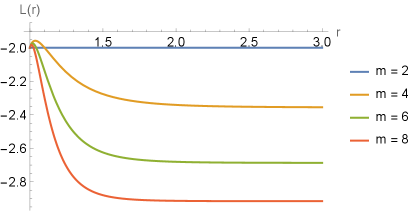
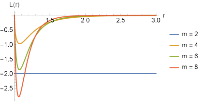
In Fig.4 , we have the plot of the Lagrangian as a function of $r$, where we can see a similar behavior for all $m>2$, in which $\mathcal{L}(r)\to$ constant for $r\to\infty$.

We can use the equation (32) to invert the Lagrangian equation and write it in terms of the invariant $\mathcal{F}$, from which we get

	$\displaystyle\mathcal{L(F)}=$	$\displaystyle\frac{2}{b_{0}^{2}[(s\mathcal{F}^{-1/4})^{m}-1]^{2/m}}\left\{1-\frac{(m-2)}{m}\left(\frac{\mathcal{F}^{1/2}}{s^{2}}\right)^{m}-\frac{2}{m}\left(\frac{\mathcal{F}^{1/4}}{s}\right)^{m}-\frac{\mathcal{F}^{1/2}}{s^{2}}\left[\left(\frac{s}{\mathcal{F}^{1/4}}\right)^{m}-1\right]^{2/m}\right.$
		$\displaystyle\left.+\frac{2(m-1)}{m}\left[1-\left(\frac{s}{\mathcal{F}^{1/4}}\right)^{m}\right]\,\,_{2}F_{1}\left(2,1-\frac{2}{m},2-\frac{2}{m},1-\left(\frac{s}{\mathcal{F}^{1/4}}\right)^{m}\right)\right\},$		(44)

where

$$s=\frac{(2q_{m}^{2})^{1/4}}{b_{0}}.$$

(45)

As a simplification, we can also define the quantity

$$\mathcal{G}=\frac{\mathcal{F}^{1/4}}{s},$$

(46)

so that in terms of $\mathcal{G},$ we have

	$\displaystyle\mathcal{L(G)}=$	$\displaystyle\frac{2}{b_{0}^{2}(\mathcal{G}^{-m}-1)^{2/m}}\left\{1-\frac{(m-2)}{m}\mathcal{G}^{2m}-\frac{2}{m}\mathcal{G}^{m}-\mathcal{G}^{2}(\mathcal{G}^{-m}-1)^{2/m}\right.$
		$\displaystyle\left.+\frac{2(m-1)}{m}(1-\mathcal{G}^{-m})\,\,_{2}F_{1}\left(2,1-\frac{2}{m},2-\frac{2}{m},1-\mathcal{G}^{-m}\right)\right\}.$		(47)

It is easy to see that for $m=2$ we recovered the usual Ellis-Bronnikov case, for which the field source is just a phantom free scalar field. That is, for $m=2$, we have $V(\phi)=1/b_{0}^{2}$ and $\mathcal{L(F)}=-2/b_{0}^{2}$. By substituting this in the action (26) we get

$$S(m=2)=\int d^{4}x\left(R-2\epsilon g^{\mu\nu}\partial_{\mu}\phi\partial_{\nu}\phi+\frac{2}{b_{0}^{2}}-\frac{2}{b_{0}^{2}}\right)=\int d^{4}x\left(R-2\epsilon g^{\mu\nu}\partial_{\mu}\phi\partial_{\nu}\phi\right),$$

(48)

that is, for $m=2$, the action reduces to the action of a free scalar field, as expected.

Alternatively, instead of considering a radial magnetic field generated by a magnetic monopole, we can consider a radial electric field, so that now the non-zero components of the electromagnetic tensor $F_{\mu\nu}$ are given by $F^{tr}=-F^{rt}=E(r)$. With this, the invariant $\mathcal{F}$ is now given by

$$\mathcal{F}=-\frac{2E(r)^{2}}{\left(1-\frac{b(r)}{r}\right)}.$$

(49)

Also, using the equation (31) we can write the electric field as

$$E(r)=\frac{q_{e}}{r^{2}\mathcal{L_{F}}}\sqrt{1-\frac{b(r)}{r}},$$

(50)

where $q_{e}$ is the electric charge.

With this, the tensor energy momentum associated with NED is given by

$$T[\mathcal{F}]^{\nu}_{\mu}=\frac{1}{2}\text{diag}\left(\mathcal{L}+\frac{4E(r)^{2}\mathcal{L_{F}}}{1-\frac{b(r)}{r}},\mathcal{L}+\frac{4E(r)^{2}\mathcal{L_{F}}}{1-\frac{b(r)}{r}}\mathcal{L},\mathcal{L}\right)$$

(51)

Here we proceed analogously to the magnetic case to find the scalar field and the associated potential, which are given by the same expressions (37) and (III.2) as the magnetic case.

Finally, from Einstein’s equation $(\theta,\theta)$ we get

$$L(r)=\frac{b(r)-rb^{\prime}(r)}{2r^{3}}-V(r)-\left(1-\frac{b(r)}{r}\right)\phi^{\prime}(r)^{2}.$$

(52)

Finally, substituting $\phi(r)$ and $V(r)$, we find that the Lagrangian is given by

$$\mathcal{L}(r)=-2\frac{(m-1)(m-2)b_{0}^{m}(r^{m}-b_{0}^{m})^{1-2/m}}{mr^{2m}}-\frac{4(m-1)(r^{m}-b_{0}^{m})^{1-2/m}}{mb_{0}^{m}}\,_{2}F_{1}\left[2,1-\frac{2}{m},2-\frac{2}{m},1-\frac{r^{m}}{b_{0}^{m}}\right].$$

(53)

Finally, from the equation $(r,r)$ we can solve for $\mathcal{L}_{F}$, since the electric field in terms of $\mathcal{L}_{F}$ is given in (50). By doing this, we get

$$\mathcal{L_{F}}(r)=-\frac{2q_{e}^{2}}{r^{2}[1-r^{2-2m}(r^{m}+(m-2)b_{0}^{m})(r^{m}-b_{0}^{m})^{1-2/m}]}.$$

(54)

In Fig.5 we have the plot of the Lagrangian $\mathcal{L}$ as a function of $r$. It is worth noting that, as usually happens in the electrical case, it is not possible to write $\mathcal{L}$ as an explicit function of $\mathcal{F}$, since $\mathcal{F}$ depends on a non-trivial form of $r$. In addition, it is possible to see that, as in the magnetic case, the Lagrangian tends to a constant for asymptotic values of $r$; However, for small values of $r$, $\mathcal{L}(r)$ diverges in the electric case, in contrast to the magnetic case, in which $\mathcal{L}(r)$ tends to a constant to $r\to 0$.

Finally, the expression for the electric field is given by

$$E(r)=\frac{(r^{m}-b_{0}^{m})^{1-3/m}}{2q_{e}r^{m+1}}\left[r^{4}-b_{0}^{2m}(m-2)r^{4-2m}+b_{0}^{m}(m-3)r^{4-m}-r^{2}(r^{m}-b_{0}^{m})^{2/m}\right].$$

(55)

This electric field is obviously not Coulombian. On the limit $r\to\infty$

$$E(r)\sim\left(\frac{b_{0}}{r}\right)^{m},$$

(56)

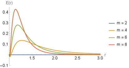
which demonstrates that the decay of the $E(r)$ field is faster the higher the value of $m$, which is in agreement with the diagram in Fig.1, which shows that the geometry tends to be flat faster as we increase the value of $m$. In the graph of Fig.6 we have the behavior of the electric field for different values of $m$, where we see that, for $r\to 0$, the electric field does not have a divergent behaviour.

References

- (1) M. S. Morris and K. S. Thorne, Am. J. Phys. 56, 395-412 (1988)
- (2) C. Bambi and K. Freese, Phys. Rev. D 79, 043002 (2009) [arXiv:0812.1328 [astro-ph]].
- (3) N. Ortiz, O. Sarbach and T. Zannias, Phys. Rev. D 92, no.4, 044035 (2015) [arXiv:1505.07017 [gr-qc]].
- (4) R. Shaikh, P. Kocherlakota, R. Narayan and P. S. Joshi, Mon. Not. Roy. Astron. Soc. 482, no.1, 52-64 (2019) [arXiv:1802.08060 [astro-ph.HE]].
- (5) C. Bambi, Phys. Rev. D 87, 107501 (2013) [arXiv:1304.5691 [gr-qc]].
- (6) M. Guerrero, G. J. Olmo, D. Rubiera-Garcia and D. S. C. Gómez, JCAP 08 (2021), 036 doi:10.1088/1475-7516/2021/08/036 [arXiv:2105.15073 [gr-qc]].
- (7) M. Azreg-Aïnou, JCAP 07, 037 (2015) [arXiv:1412.8282 [gr-qc]].
- (8) V. A. Ishkaeva and S. V. Sushkov, Phys. Rev. D 108, no.8, 084054 (2023) [arXiv:2308.02268 [gr-qc]].
- (9) M. Alloqulov, F. Atamurotov, A. Abdujabbarov, B. Ahmedov and V. Khamidov, Chin. Phys. C 48, no.2, 025104 (2024)
- (10) R. Shaikh, Phys. Rev. D 98, no.2, 024044 (2018) [arXiv:1803.11422 [gr-qc]].
- (11) K. Akiyama et al. [Event Horizon Telescope], Astrophys. J. Lett. 875, L1 (2019) [arXiv:1906.11238 [astro-ph.GA]].
- (12) K. Akiyama et al. [Event Horizon Telescope], Astrophys. J. Lett. 930, no.2, L12 (2022) [arXiv:2311.08680 [astro-ph.HE]].
- (13) V. De Falco, E. Battista, S. Capozziello and M. De Laurentis, Phys. Rev. D 101, no.10, 104037 (2020) [arXiv:2004.14849 [gr-qc]].
- (14) V. De Falco and S. Capozziello, Phys. Rev. D 108, no.10, 104030 (2023) [arXiv:2308.05440 [gr-qc]].
- (15) S. Jana, V. Sharma and S. Ghosh, [arXiv:2411.10804 [gr-qc]].
- (16) E. Franzin, S. Liberati, J. Mazza, A. Simpson and M. Visser, JCAP 07 (2021), 036 doi:10.1088/1475-7516/2021/07/036 [arXiv:2104.11376 [gr-qc]].
- (17) J. Furtado and G. Alencar, Universe 8 (2022) no.12, 625 doi:10.3390/universe8120625 [arXiv:2210.06608 [gr-qc]].
- (18) C. F. S. Pereira, A. R. Soares, M. V. d. S. Silva, R. L. L. Vitória and H. Belich, [arXiv:2505.12577 [gr-qc]].
- (19) G. Alencar, A. Duran-Cabacés, D. Rubiera-Garcia and D. Sáez-Chillón Gómez, Phys. Rev. D 111 (2025) no.10, 104020 doi:10.1103/PhysRevD.111.104020 [arXiv:2501.03909 [gr-qc]].
- (20) H. G. Ellis, J. Math. Phys. 14, 104-118 (1973)
- (21) K. A. Bronnikov, Acta Phys. Polon. B 4, 251-266 (1973)
- (22) S. Kar, S. Minwalla, D. Mishra and D. Sahdev, Phys. Rev. D 51, 1632-1638 (1995)
- (23) A. Simpson and M. Visser, JCAP 02, 042 (2019) [arXiv:1812.07114 [gr-qc]].
- (24) T. M. Crispim, M. Estrada, C. R. Muniz and G. Alencar, JCAP 10, 063 (2024) [arXiv:2405.08048 [hep-th]].
- (25) T. M. Crispim, G. Alencar and M. Estrada, [arXiv:2407.03528 [gr-qc]].
- (26) A. Lima, G. Alencar and D. Sáez-Chillon Gómez, Phys. Rev. D 109, no.6, 064038 (2024) [arXiv:2307.07404 [gr-qc]].
- (27) A. M. Lima, G. M. de Alencar Filho and J. S. Furtado Neto, Symmetry 15, no.1, 150 (2023) [arXiv:2211.12349 [gr-qc]].
- (28) K. A. Bronnikov, Phys. Rev. D 110, no.2, 024021 (2024) [arXiv:2404.14816 [gr-qc]].
- (29) K. A. Bronnikov and R. K. Walia, Phys. Rev. D 105, no.4, 044039 (2022) [arXiv:2112.13198 [gr-qc]].
- (30) G. Alencar, K. A. Bronnikov, M. E. Rodrigues, D. Sáez-Chillón Gómez and M. V. de S. Silva, Eur. Phys. J. C 84, no.7, 745 (2024) [arXiv:2403.12897 [gr-qc]].
- (31) A. Lima, G. Alencar, R. N. Costa Filho and R. R. Landim, Gen. Rel. Grav. 55, no.10, 108 (2023) [arXiv:2306.03029 [gr-qc]].
- (32) K. A. Bronnikov, M. E. Rodrigues and M. V. de S. Silva, Phys. Rev. D 108, no.2, 024065 (2023) [arXiv:2305.19296 [gr-qc]].
- (33) M. E. Rodrigues and M. V. d. S. Silva, Phys. Rev. D 107, no.4, 044064 (2023) [arXiv:2302.10772 [gr-qc]].
- (34) J. Bardeen, Proc. 5th Int. Conf. on Gravitation and the Theory of Relativity, p. 87 (1968).
- (35) M. E. Rodrigues and M. V. de Sousa Silva, JCAP 06, 025 (2018) [arXiv:1802.05095 [gr-qc]].
- (36) P. Cañate and F. H. Maldonado-Villamizar, Phys. Rev. D 106, no.4, 044063 (2022) [arXiv:2202.12463 [gr-qc]].
- (37) P. Cañate, Phys. Rev. D 110, no.8, 084030 (2024) [arXiv:2409.15510 [gr-qc]].
- (38) P. Dutta Roy, S. Aneesh and S. Kar, Eur. Phys. J. C 80, no.9, 850 (2020) [arXiv:1910.08746 [gr-qc]].
- (39) P. D. Roy, Eur. Phys. J. C 82, no.8, 673 (2022) [arXiv:2110.05019 [gr-qc]].
- (40) V. Sharma and S. Ghosh, Eur. Phys. J. C 82, no.8, 702 (2022) [arXiv:2205.05973 [gr-qc]].
- (41) V. Sharma and S. Ghosh, Eur. Phys. J. Plus 137, no.8, 881 (2022) [arXiv:2205.08865 [gr-qc]].
- (42) V. Sharma and S. Ghosh, Eur. Phys. J. C 81, no.11, 1004 (2021) [arXiv:2111.07329 [gr-qc]].
- (43) N. Godani and S. Kala, Int. J. Mod. Phys. D 32, no.10, 2350067 (2023)
- (44) R. C. Muniz and R. V. Maluf, [arXiv:2203.09263 [gr-qc]].
- (45) M. Nilton, J. Furtado, G. Alencar and R. R. Landim, Annals Phys. 448, 169195 (2023) [arXiv:2203.08860 [gr-qc]].
- (46) T. F. de Souza, A. C. A. Ramos, R. N. Costa Filho and J. Furtado, Phys. Rev. B 106, no.16, 165426 (2022)
- (47) P. Mach, E. Malec and J. Karkowski, Phys. Rev. D 88 (2013) no.8, 084056 doi:10.1103/PhysRevD.88.084056 [arXiv:1309.1252 [gr-qc]].
- (48) R. Yang, Phys. Rev. D 92 (2015) no.8, 084011 doi:10.1103/PhysRevD.92.084011 [arXiv:1504.04223 [gr-qc]].
- (49) S. Bahamonde and M. Jamil, Eur. Phys. J. C 75 (2015), 508 doi:10.1140/epjc/s10052-015-3734-9 [arXiv:1508.07944 [gr-qc]].
- (50) A. K. Ahmed, M. Azreg-Aïnou, S. Bahamonde, S. Capozziello and M. Jamil, Eur. Phys. J. C 76 (2016) no.5, 269 doi:10.1140/epjc/s10052-016-4118-5 [arXiv:1602.03523 [gr-qc]].
- (51) M. Azreg-Aïnou, A. K. Ahmed and M. Jamil, Class. Quant. Grav. 35 (2018) no.23, 235001 doi:10.1088/1361-6382/aae997 [arXiv:1809.03320 [gr-qc]].
- (52) J. C. S. Neves and A. Saa, Annals Phys. 420 (2020), 168269 doi:10.1016/j.aop.2020.168269 [arXiv:1906.03718 [gr-qc]].
- (53) G. Panotopoulos, A. Rincon and I. Lopes, Annals Phys. 433 (2021), 168596 doi:10.1016/j.aop.2021.168596 [arXiv:2108.12984 [gr-qc]].
- (54) A. Rueda and E. Contreras, Annals Phys. 459 (2023), 169540 doi:10.1016/j.aop.2023.169540 [arXiv:2311.08344 [gr-qc]].
- (55) L. Combi, H. Yang, E. Gutierrez, S. C. Noble, G. E. Romero and M. Campanelli, Phys. Rev. D 109 (2024) no.10, 103034 doi:10.1103/PhysRevD.109.103034 [arXiv:2405.06900 [astro-ph.HE]].
- (56) U. Debnath, Eur. Phys. J. C 75 (2015), 129 doi:10.1140/epjc/s10052-015-3349-1 [arXiv:1503.01645 [gr-qc]].
- (57) K. A. Bronnikov, Particles 1, no.1, 56-81 (2018) [arXiv:1802.00098 [gr-qc]].