Finite perturbation theory for the relativistic Coulomb problem
Abstract
We present a novel form of relativistic quantum mechanics and demonstrate how to solve it using a recently derived unitary perturbation theory, within partial wave analysis. The theory is tested on a relativistic problem, with two spinless, equal mass particles, in which the interaction is entirely given by a Coulomb potential. As such, it is not meant to reproduce experimental results for the scattering of two electrons, but is intended as a test of our calculation methods. We find that this perturbation theory gives finite results at second order. This is unlike other versions of perturbation theory, which find divergent results at second and all higher orders. We calculate differential cross sections in the nonrelativistic regime, where we find excellent agreement with the Rutherford formula. Then, well into the relativistic regime, we find differential cross sections with similar shapes to the Møller formula and differing from that formula by less than an order of magnitude.
I Introduction
There are two aims of this paper. The first is to apply a novel perturbation theory to the problem of the Coulomb scattering of two (spinless) charged particles. This problem has been treated before with other forms of perturbation theory, with the well-known result that all corrections at second and higher order diverge (Dalitz [1]). The reason, in this context, is that certain integrals over particle separation do not converge because the Coulomb potential falls off insufficiently fast at large particle separation. We note that even the first-order result is problematic (Collas [2]).
The new method used here (Hoffmann [3]) involves working in momentum space and a prescription to use principal part integration on the momentum integrals. We will find that this procedure produces finite results in agreement with expectations when applied to the Coulomb potential.
The other aim of this paper is to show that some features of relativity can be easily incorporated into our model. For our purposes, relativity gives a different dependence of single-particle energy on momentum from the nonrelativistic form, and can add new terms to the interaction. For the latter, an example is the emergence of the spin-orbit coupling term when the Foldy-Wouthuysen transformation is applied to the Dirac equation (Foldy and Wouthuysen [4]). In our model, we will introduce the relativistic form of the single-particle energy. We will consider an entirely Coulomb potential in this spinless case.
We note that relativity constrains measurements made in different frames, but does not tell us about measurements in one frame. The position profile of a porcupine depends on how that animal has grown, and varies from animal to animal. Relativity tells us only how a moving frame would measure a changed porcupine profile. We will propose that there must be a four-component potential operator that transforms as a four-vector to have a covariant relativistic quantum mechanics. We will find that in a centre of mass (CM) frame, the spatial components must vanish. The form of the potential in a CM frame is arbitrary for our considerations, but is determined by the model of microscopic interactions in quantum electrodynamics (Weinberg [5]). Future work will define these potentials and explore the consequences.
Throughout this paper, we use Heaviside-Lorentz units, in which
II Finite, relativistic, perturbation theory
II.1 Relativistic Schrödinger equations
We are motivated by the success of nonrelativistic quantum mechanics, in which the total Hamiltonian is written as the sum of a free part and a part responsible for interaction (a potential ):
| (1) |
Here indicates free, indicates interacting, hats indicate operators.
Thus we propose for relativistic quantum mechanics the four equations ()
| (2) |
Here the potential of nonrelativistic quantum mechanics becomes the zero component of what must transform as a four-vector, as do the components of and to guarantee relativistic covariance. This is
| (3) |
where is the unitary representation of a general Lorentz transformation, and is the corresponding coordinate transformation matrix. For processes involving photons, we assert that must be gauge invariant to arrive at physical results independent of the gauge.
For the scattering of two spinless “electrons”, we choose as free basis vectors In the CM frame, these are defined in terms of the individual momentum eigenvectors as
| (4) |
Then a boost takes them to general four-momentum
| (5) |
We can ignore the total linear momentum, by using the normalization
| (6) |
which has no consequences.
These are eigenvectors of total four-momentum They are also eigenvectors of and where is the total angular momentum (which in this case is entirely orbital angular momentum) in the CM frame (where ). In the more general case, where the two particles can be any combination of electrons, positrons and photons, the basis vectors take the form where and are the quantum numbers associated with the total CM-frame angular momentum, and and are the CM-frame helicities of the two particles.
It is advantageous to work in momentum space, where the square roots in the single-particle energies, pose no problem. At this point there is no need to introduce spacetime coordinates for the two particles. Note that to see a potential with spacetime dependence requires taking matrix elements between two state vectors, at least one of which has spacetime dependence.
Corresponding to each free basis vector is an interacting basis vector that solves the Schrödinger equations (eq. (2)). We will explore this correspondence shortly.
We take matrix elements
| (7) |
which reduce to
| (8) |
a set of integral equations. We ensure that the free basis vectors are orthonormalized and complete so that we can insert the completeness relation as we have just done.
II.2 Simplification in the centre of mass frame
A simplification is possible. We will find below that it is possible to define a unitary transformation that relates free and interacting basis vectors with the same quantum numbers:
| (9) |
Note that in the quantum electrodynamics formalism (Weinberg [5]), the electron is given a free mass different from its mass after including electromagnetic interactions. But the difference of these masses is calculated to diverge and only the interacting mass is observable. As we will see, the correspondence proposed here produces no divergences.
The transformation of operators that gives the same expectation values is
| (10) |
Note that we will have similar relations for the transformation of rotation generators () and boost generators ():
| (11) |
Consequently, if
| (12) |
then
| (13) |
So, from eq. (), we see the vanishing of the matrix elements of the three-vector part of the potential, in the one CM frame that is the same in the free and interacting theories:
| (14) |
In what follows, we will perform calculations only in the CM frame, knowing that we could transform differential cross sections to other frames, if necessary.
II.3 Translational and rotational invariance
We define We know
| (15) |
by translational invariance, so we can remove all reference to the three-momenta and arrive at the simplified equation in the CM frame (understanding throughout)
| (16) |
We are considering the case of a potential that is rotationally invariant (). Thus, by the Wigner-Eckhart theorem (Messiah [6]), the matrix elements take the form
| (17) |
Furthermore, if the potential is rotationally invariant, we expect that the free to interacting transformation will also be rotationally invariant, preserving the quantum numbers and . A further reduction, ignoring gives
| (18) |
II.4 Eigenvectors of particle separation
The phase shifts that we want to calculate come from the asymptotic behaviour of interacting position wavefunctions as the separation, of the two particles increases without bound. Thus we need to construct eigenvectors of the operator associated with this separation. Note that we cannot here use the techniques of nonrelativistic quantum mechanics, where the kinetic energy depends quadratically on the momentum, to form the total linear momentum and the relative momentum.
We consider two different individual particle translations applied to a free individual momentum eigenvector:
| (19) |
This transformation changes the separation of the two particles by but leaves the average position unchanged. So we define simultaneous eigenvectors of separation and total three-momentum as
| (20) |
noting that
| (21) |
and commute.
Then we form eigenvectors of the magnitude of the separation and of orbital angular momentum,
| (22) |
where the argument of the spherical harmonic is here a unit vector, not an operator. We note that defined in the CM frame also commutes with
Note that we will only be requiring these basis vectors for the special case where is the separation and label the orbital angular momentum, both in the CM frame. Note also that these basis vectors will have calculable but very complicated Lorentz transformation properties, as with any position eigenvectors.
If we choose the orthonormalization
| (23) |
then we find
| (24) |
We find the relation between eigenvectors of momentum magnitude and eigenvectors of separation magnitude:
| (25) |
in terms of the free spherical waves, familiar from partial wave analysis (Messiah [6]). This motivates our definition for the interacting case,
| (26) |
in terms of the interacting wavefunctions,
Note that the position eigenvectors are common to the free and interacting theories. We do not define interacting position eigenvectors.
II.5 Unitary perturbation theory
A unitary transformation connecting the free and interacting theories, in the nonrelativistic case, was introduced in Hoffmann [3], and a perturbation series was developed to second order in the coupling strength. Only minor changes are needed to treat the relativistic case.
In the CM frame, the total energies are
| (27) |
where is the magnitude of both single-particle momenta. Then a change of quantum numbers to eq. (18) gives
| (28) |
The normalizations are
| (29) |
We expand the unitary transformation to second order in :
| (30) |
where
| (31) |
Then we solve the equation
| (32) |
order by order, with . The results are
| (33) |
The solutions for the matrix elements of and are
| (34) |
and
| (35) |
where
| (36) |
Also
| (37) |
The symbol indicates that when these expressions are integrated over momentum, the principal part prescription (also known as finding the Cauchy principal value) must be used. We have seen in (Hoffmann [3]) that use of this prescription eliminates divergences and give results in agreement with an exactly solvable model.
Then the interacting position separation wavefunction to second order is
| (38) |
II.6 Calculation of phase shifts
For the Coulomb potential in the CM frame, the matrix elements are
| (39) |
with Both sections of this function are singular at Close to the singularity, with for small we find the approximation (Olver et al. [7], their eq. (15.8.10))
| (40) |
with
| (41) |
and
| (42) |
known as Euler’s constant. Here is the logarithmic derivative of the gamma function (Gradsteyn and Ryzhik [8], their section 8.36).
These functions have the property that they have a singular point but are integrable across the singularity. This will be sufficient for the principal part integrals to converge to finite values.
To find the asymptotic form of in eq. (38), we first use the asymptotic forms of the free spherical waves (Messiah [6])
| (43) |
For the first-order term (with )
| (44) |
We review the rules we learned from the similar case in Hoffmann [3]:
-
•
For the and integrals, the contributions from will vanish asymptotically like since the integrand has no singularities on that region and the sinusoids oscillate rapidly.
-
•
The factor acts as a delta function. When combined with the singularity of we have (with )
(45) -
•
There is no delta function in the integral containing On only integrands even in will survive the principal part integration. In this integrand, there will be factors of the form with and and We note that the first of these terms and are finite at the origin. So we consider integrals of the form
(46) where This integral vanishes at and decreases like for
Thus we find (with where is the relativistic velocity magnitude for either of the particles)
| (47) |
with
| (48) |
Here corresponds to the parameter defined in the nonrelativistic case, with the reduced mass in this case. We will find that our perturbation series is in powers of rather than of
We use similar methods for the second-order terms, employing the four rules
| (49) |
all for having no singularities. We evaluate the terms in eq. (38) as written, performing each integral before the integral. We find that changing the order of the double momentum integrals changes some of the terms, but the total is invariant. An ambiguity remains. Using partial fractions to cancel some terms gives a different final result. We suspect this is because doing this changes the set of poles in the integrands. This matter is under further investigation.
We find the result
| (50) |
We note that the term proportional to has the correct form required by unitarity at this order. The last term is
| (51) |
where
| (52) |
at
III Calculation of differential cross sections
We use the results of Hoffmann [9], where we considered the scattering of a single-particle wavepacket from a Coulomb potential. A slight modification of the differential cross section formula, here in the CM frame, with the resulting form shown here, was necessary to treat the scattering of two particles,
| (53) |
The wavepacket treatment makes the sum in eq. (53) converge, even for It was previously thought that partial wave analysis was not applicable to the Coulomb potential, as the sum over in eq. (53) diverges for all scattering angles if the convergence factor is not present. This treatment introduces another physical parameter,
| (54) |
where is the standard deviation of the Gaussian probability density in momentum space of all the initial and final wavepackets. The standard deviation in position space at is with In practice, we choose In the nonrelativistic case, we found generally excellent agreement with the Rutherford formula (Rutherford [10]),
but deviations close to that are influenced by the choice of
In eq. (53), the Coulomb phase shifts, have been replaced by the phase shifts of our model to second order. Here
| (55) |
measures the time delay (positive) or advancement (negative) over the time, of the experiment, relative to free evolution. The wavepacket centres are separated by at the start of the experiment. As discussed in Hoffmann [9], the choice gives an initial separation that grows as is decreased, while wavepacket spreading is minimal over the course of the experiment. The quantities
| (56) |
that influence this time shift involve the logarithmic phase, from which has been removed in the definition
| (57) |
The approximation in eq. (56) will be sufficient for our purposes, as we will mostly be considering small
In what follows, we evaluate the phase shifts numerically and insert them into the cross section formula, sum the series numerically and take the modulus-squared.
IV Numerical results
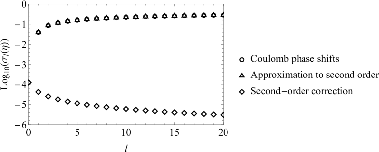
First we calculate the phase shifts and compare them to the Coulomb phase shifts in the nonrelativistic regime (, , ), where we expect agreement. We find the results plotted in fig. 1. The second-order corrections are seen to be much smaller than the Coulomb phase shifts. Note that the exact and approximate phase shifts are negative at , so are not included in this logarithmic plot.
That the second-order corrections were calculable and finite achieves the first goal of this paper. That the corrections were small is as it should be, since the first-order result gave a good approximation to the Coulomb phase shifts.
As could be expected from this result, the plots of the model differential cross section and the Rutherford formula were visually indistinguishable, except close to for this nonrelativistic choice of momentum. We took small but slowly varying, up to The profile in at peaked very near
Into the relativistic regime, we plotted the model differential cross section (just to first order) at for a range of momenta from about to in fig. (2), compared with the Rutherford differential cross section.

We see agreement with the Rutherford differential cross section at low momenta and a distinct deviation at higher momenta. One reason that the relativistic result would be larger than the Rutherford result is that the coupling strength in the former can be no lower than since while the nonrelativistic form has a lower bound of zero.
At () we plotted the differential cross section as a function of angle, again comparing with the Rutherford result. This is shown in fig. (3). At the profile peaked very near We note that the model cross section was seen to take a large but finite value at while the Rutherford formula diverges there. This finiteness was discussed in Hoffmann [9].

At higher momenta, a more meaningful comparison is with the Møller formula (Itzykson and Zuber [11]). This is the differential cross section derived from tree-level quantum electrodynamics for the scattering of two electrons. To imitate a spinless system, it has been averaged over initial spins and summed over final spins. The formula is
To make the comparison, we could not antisymmetrize these two fictitious bosons. Instead, to have a definite particle exchange symmetry, we symmetrized our model scattering amplitude, treating the two particles as identical. This involved inserting a factor in the sum over that defines the scattering amplitude.
For we plotted the angular dependence of the model cross section along with that of the Møller formula and the Rutherford formula, in fig. (4).

For the scattering angle we plotted the dependence on momentum of the model cross section and the Møller formula, in fig. (5).

It is remarkable that our model lacks many of the essential features of the electron-electron scattering problem, other than the Coulomb potential, yet shows quite good agreement with the Møller formula. Note that the symmetrized model cross section no longer converges to the Rutherford formula at nonrelativistic energies. Instead, it must converge to a symmetric cross section that evidently has some features in common with the Rutherford formula. We recall that the unsymmetrized cross section was seen to converge to the unsymmetrized Rutherford formula. It is then puzzling why the Møller formula converges to a cross section that has no definite particle exchange symmetry.
V Conclusions
There were two aims of this paper. One was to use a novel perturbation theory on the Coulomb potential and show that finite results could be obtained. In comparison, other forms of perturbation theory find infinite results at second and all higher orders. This aim was achieved using only one rule that was imposed rather than derived: the requirement that principal part integration be used on the momentum integrals.
The other aim was to show that it is possible to construct a theory that is relativistic and quantum-mechanical, but not quantum field-theoretic and not the wave mechanics of a single particle in a potential. This was achieved by working in momentum space, where the relativistic dependence of single-particle energy on momentum can be easily introduced. We found that the three-vector part of the four-potential must vanish in the centre of mass frame. That leaves an arbitrary zero component, at first sight not constrained by relativity. The further success of this method depends on being able to choose a CM-frame potential that reproduces experimental results.
The model of a Coulomb potential in the centre of mass frame was not intended to provide a full description of the scattering of two electrons. It was intended only as a proof of principle for the method considered. There are other terms that contribute to the scattering of two electrons. In a future work, we will include those terms, with the expectation of finite results.
Also in a future work, we will analyze the forms of the terms in our perturbation theory, to see if it is possible to prove finiteness at higher orders.
References
- Dalitz [1951] R. H. Dalitz, Proc. Roy. Soc. Lond. A: Math., Phys. and Eng. Sci. 206, 509 (1951).
- Collas [2021] P. Collas, arXiv:2102.13105 (2021).
- Hoffmann [2021] S. E. Hoffmann, J. Math. Phys. 62, 032105 (2021).
- Foldy and Wouthuysen [1950] L. L. Foldy and S. A. Wouthuysen, Phys. Rev. 78, 29 (1950).
- Weinberg [2012] S. Weinberg, The Quantum Theory of Fields, Vol. 1 (Cambridge University Press, N.Y., 2012).
- Messiah [1961] A. Messiah, Quantum Mechanics, Vol. 1 and 2 (North-Holland, Amsterdam and John Wiley and Sons, N.Y., 1961).
- Olver et al. [2020] F. W. J. Olver et al., “NIST Digital Library of Mathematical Functions,” http://dlmf.nist.gov/, Release 1.0.25 of 2019-12-15 (2020).
- Gradsteyn and Ryzhik [1980] I. S. Gradsteyn and I. M. Ryzhik, Tables of Integrals, Series and Products, corrected and enlarged ed. (Academic Press, Inc., San Diego, CA, 1980).
- Hoffmann [2017] S. E. Hoffmann, J. Phys. B: At. Mol. Opt. Phys. 50, 215302 (2017).
- Rutherford [1911] E. Rutherford, Phil. Mag. Series 6, vol. 21, 669 (1911).
- Itzykson and Zuber [1980] C. Itzykson and J.-B. Zuber, Quantum Field Theory, 1st ed. (McGraw-Hill Inc., 1980).