Finite Temperature Casimir Effect of Scalar Field: Revisit and New Results

The Casimir effect serves as compelling evidence for quantum fluctuations in the vacuum. Specifically, the quantum fluctuations of the electromagnetic field induce an attractive Casimir interaction between two parallel, electrically neutral metal plates [1, 2, 3, 4, 5], which is mathematically expressed as $-{\pi^{2}c\hbar}/{240a^{4}}$ at zero temperature, where $a$ denotes the separation between the plates. This interaction is significant in the micron to nanometer scale, profoundly influencing the design, functionality, and performance of micro- and nano-electromechanical devices. Over the past two decades, substantial experimental advancements have been achieved in the study of the Casimir effect, including the exploration of repulsive Casimir interactions [6, 7, 8], the critical Casimir effect [9, 10, 11, 12, 13, 14], the dynamical Casimir effect [15, 16, 17, 18], and the Casimir-Lifshitz torque [19], among others. Additionally, theoretical investigations have proliferated in various directions. Repulsive Casimir interactions have been proposed in system with special geometry [20], metamaterials [21, 22], a series of topological materials [23, 24, 25, 26], and chiral substances [27]. Furthermore, Casimir interactions mediated by alternative entities, other than virtual photons, such as gravity [28], massless fermions [29], neutrinos [30], phonons [31], and magnons [32], have garnered considerable attention.

Despite these significant advancements, a fundamental theoretical challenge known as the thermal Casimir problem remains unresolved, as recently reviewed by V. M. Mostepanenko [33] and named the Casimir puzzle and the Casimir conundrum, and has been extensively researched over the last two decades, see, e.g., Refs. [34, 35, 36, 37, 38, 39, 40]. The commonly employed Drude model description of metal and an inclusion of direct current conductivity in dielectric materials appear to be inherently incompatible with the description of the Casimir effect provided by Lifshitz theory. Detailed investigations reveal marked discrepancies between the predictions of the Drude model and experimental measurements. The Drude model’s representation of metal results in a negative entropy that contravenes the Nernst heat theorem [41]. In this study, we revisit the longstanding problem of the finite temperature Casimir effect in one-dimensional and three-dimensional scalar fields. Through meticulous calculations, we derive analytical expressions for the Gibbs energy of these fields under Dirichlet boundary conditions (i.e., ideal metal boundary conditions). The black body radiation of fields in free space and the divergent terms in the high-temperature limit are two commonly utilized counterterms in previous investigations. Our exact solutions reveal that both these two types of counterterms are problematic, leading to the emergence of negative entropy in these scenarios.

Consider the scalar field described by the following equation,

$$\left(\frac{\partial^{2}}{\partial{t}^{2}}-v^{2}\frac{\partial^{2}}{\partial{x}^{2}}\right)\phi(x,t)=0,$$

(1)

where $v$ is the velocity of the scalar field. After the quantization of field, we can get the eigenenergy of the field with Dirichlet boundary condition, $\phi(0,t)=\phi(a,0)=0$,

$$E_{n}(l)=\left(n+\frac{1}{2}\right)\hbar{v}\frac{l\pi}{a},$$

(2)

where $n=0,1,2,...$ is the particle number, $l=1,2,3,...$ describes the quantized wave vector, $k=l\pi/a$. At finite temperature, $T$, the partition function can be written as,

$$Z=\prod_{l=1}^{\infty}\sum_{n=0}^{\infty}e^{-{E_{n}(l)/T}},$$

(3)

we set the Boltzmann’s constant $k_{B}=1$ in our investigation. We can complete the summation over particle number $n$ in Eq. (3) to get,

$$Z=\prod_{l=1}^{\infty}\frac{\exp\left(-{l\pi{v}\hbar}/{2aT}\right)}{1-\exp\left(-{l\pi{v}\hbar}/{aT}\right)}.$$

(4)

The Gibbs free energy is defined as,

$$F=-T\log(Z),$$

(5)

which gives, from Eq. (4), that,

$$F=\sum_{l=1}^{\infty}\left\{\frac{l\pi{v}\hbar}{2a}+T\log\left[1-\exp\left(-\frac{l\pi{v}\hbar}{aT}\right)\right]\right\}.$$

(6)

The two terms in this equation have significant differences. The first term is related to the vacuum state, it is divergent but temperature independent, the second term is related to the thermal fluctuation of field, it is temperature dependent but convergent. Using the Riemann $\zeta$-function regularization, $\sum_{l=1}^{\infty}l=\zeta(-1)=-1/12$, we can get,

$$F=-\frac{\pi{v}\hbar}{24a}+T\sum_{l=1}^{\infty}\log\left[1-\exp\left(-\frac{l\pi{v}\hbar}{aT}\right)\right].$$

(7)

The summation of the second term can also be carried out, which gives,

$$\sum_{l=1}^{\infty}\log\left[1-\exp\left(-\frac{l\pi{v}\hbar}{aT}\right)\right]=\frac{\pi{v}\hbar}{24aT}+\log\left[\eta\left(\frac{iv\hbar}{2aT}\right)\right],$$

(8)

where $\eta$ is the Dedekind $\eta$ function,

$$\eta(z)=q^{1/24}\prod_{n=1}^{\infty}(1-q^{n}),~{}~{}~{}(q=e^{2i\pi{z}}),$$

(9)

which is defined on the upper half complex plane ($\textrm{Re}[z]>0$), and satisfies the following modular property,

$$\eta(z)=\sqrt{\frac{i}{z}}\eta\left(-\frac{1}{z}\right).$$

(10)

Substituting the summation in Eq. (7) by Eq. (8), we find that the terms proportional to $a^{-1}$ are canceled and we get a very simple expression of the Gibbs free energy (for the Casimir effect of the one-dimensional scalar field),

$$F=T\log\left[\eta\left(\frac{iv\hbar}{2aT}\right)\right].$$

(11)

Free energy of the free space should be considered carefully. We discuss this issue and related counter terms in the following context.

The Casimir force ($P$) and the Casimir entropy ($S$) can be calculated by using the following definitions,

	$$\displaystyle P=-\frac{\partial{F}}{\partial{a}},$$		(12)
	$$\displaystyle S=-\frac{\partial{F}}{\partial{T}}.$$		(13)

We find the following analytical results,

	$$\displaystyle P=\frac{iv\hbar}{2a^{2}}\frac{\eta^{\prime}\left({iv\hbar}/{2aT}\right)}{\eta\left({iv\hbar}/{2aT}\right)},$$		(14)
	$$\displaystyle S=-\log\left[\eta\left(\frac{iv\hbar}{2aT}\right)\right]+\frac{iv\hbar}{2aT}\frac{\eta^{\prime}\left({iv\hbar}/{2aT}\right)}{\eta\left({iv\hbar}/{2aT}\right)}.$$		(15)

These exact results show that the Gibbs free energy can be written as the following classical thermal dynamical form,

$$F=Pa-TS.$$

(16)

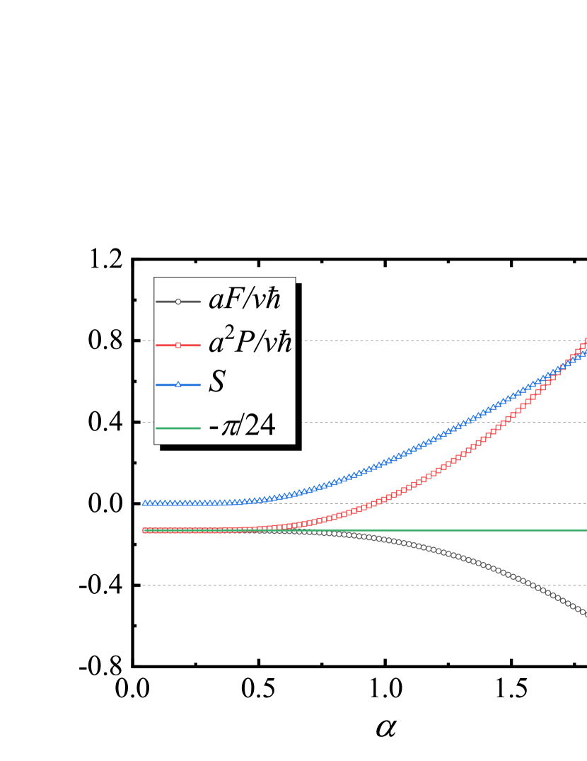
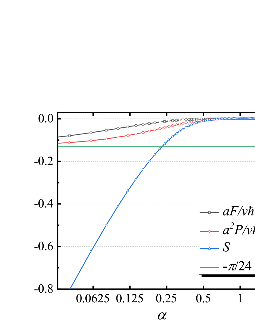
In order to get the graphical representation of free energy, force and entropy, we define the following dimensionless variable,

$$\alpha=\frac{aT}{v\hbar},$$

(17)

and rewrite the Gibbs free energy, Casimir force, and Casimir entropy in the following forms,

	$$\displaystyle\frac{a}{v\hbar}F=\alpha\log\left[\eta\left(\frac{i}{2\alpha}\right)\right],$$		(18)
	$$\displaystyle\frac{a^{2}}{v\hbar}P=\frac{i}{2}\frac{\eta^{\prime}(i/2\alpha)}{\eta(i/2\alpha)},$$		(19)
	$$\displaystyle S=-\log\left[\eta\left(\frac{i}{2\alpha}\right)\right]+\frac{i}{2\alpha}\frac{\eta^{\prime}(i/2\alpha)}{\eta(i/2\alpha)},$$		(20)

Note that

$$\lim_{\alpha\rightarrow 0}\alpha\log[\eta(i/2\alpha)]=-\frac{\pi}{24},$$

we can get the correct zero-temperature limit result,

	$$\displaystyle F(T\rightarrow 0)=-\frac{\pi}{24}\frac{v\hbar}{a},$$		(21)
	$$\displaystyle P(T\rightarrow 0)=-\frac{\pi}{24}\frac{v\hbar}{a^{2}},$$		(22)
	$$\displaystyle S(T\rightarrow 0)=0.$$		(23)

Next we consider the asymptotic behavior of Gibbs free energy, Casimir force and Casimir entropy. We first consider the low temperature limit $T\rightarrow 0$ ($\alpha\ll 1$). In this case, we should use the modular property (10) to rewrite the Gibbs free energy as follows,

$$F=T\log\left[\sqrt{\frac{2aT}{v\hbar}}\eta\left(\frac{2iaT}{v\hbar}\right)\right],$$

(24)

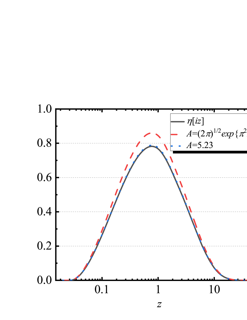
Near the zero temperature point, the Dedekind $\eta$ function can be approximated as [42, 43],

$$\displaystyle\eta(\tau)=Aq^{1/24}(1-q)^{-1/2}\exp\left[-\frac{\pi^{2}}{6(1-q)}\right],$$

(25)

where $A$ is a coefficient need to be determined, $q=e^{2i\pi{\tau}}$. Fig. 2 shows the Dedekind $\eta$ function and its approximation given in Eq. (25) with different parameters, $A=\sqrt{2\pi}e^{\pi^{2}/12}$ and $5.23$. The parameter $A=\sqrt{2\pi}e^{\pi^{2}/12}$ has a better approximation at $z\rightarrow 0$, while $A=5.23$ has a better performance in the whole domain. We choose $A=\sqrt{2\pi}e^{\pi^{2}/12}$ by considering that $S(T\rightarrow 0)=0$. Using this approximation, we can get the Gibbs free energy, Casimir force and Casimir entropy in the low temperature limit,

	$$\displaystyle\frac{a}{v\hbar}F=\alpha\left[\frac{\pi^{2}}{12}+\frac{1}{2}\log(2\pi)-\frac{\pi\alpha}{6}-\frac{\pi^{2}}{6(1-e^{-4\pi\alpha})}\right.$$
	$$\displaystyle\left.+\frac{1}{2}\log\left(\frac{2\alpha}{1-e^{-4\pi\alpha}}\right)\right],$$		(26)
	$$\displaystyle\frac{a^{2}}{v\hbar}P=-\frac{\alpha}{2}+\pi\alpha^{2}\left[\frac{1}{6}+\frac{2e^{-4\pi\alpha}}{1-e^{-4\pi\alpha}}-\frac{2\pi^{2}e^{-4\pi\alpha}}{3(1-e^{-4\pi\alpha})^{2}}\right],$$		(27)
	$$\displaystyle S=-\frac{6+6\log(2\pi)+\pi^{2}}{12}-\frac{5\pi\alpha}{3}-\frac{1}{2}\log\left(\frac{2\alpha}{1-e^{-4\pi\alpha}}\right)$$
	$$\displaystyle+\left(\frac{\pi^{2}}{6}+\frac{3+\pi^{2}}{3}2\pi\alpha\right)\frac{1}{1-e^{-4\pi\alpha}}-\frac{2\pi^{3}\alpha}{3}\frac{1}{\left(1-e^{-4\pi\alpha}\right)^{2}},$$		(28)

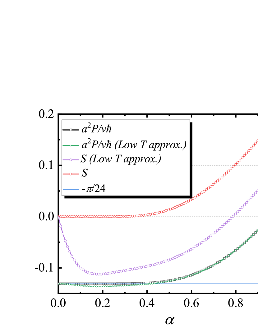
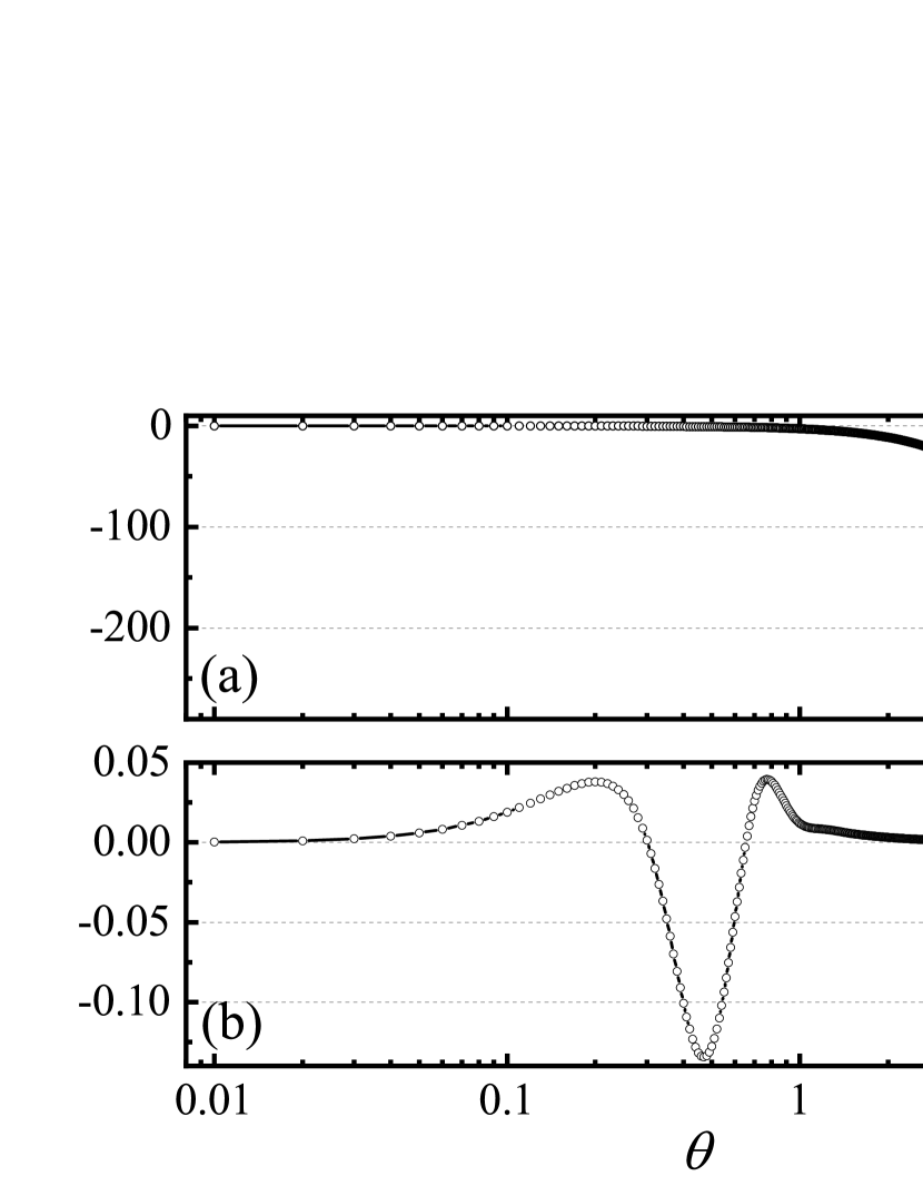
Fig. 3 shows the numerical results of these approximations (the Casimir force and the Casimir entropy under the low temperature approximation) and their exact solutions. From these plots, we may make the following conclusion that, (i) in the low temperature regime, e.g., $0<\alpha<0.20$, the thermal fluctuation of Casimir force makes the attraction to be enhanced; (ii) the Casimir entropy is negative in the low temperature regime (e.g. $0<\alpha<0.8$). However, the exact solution do not support such a conclusion. The asymptotic behavior shown in Eq. (25), is a very good approximation of the Dedekind $\eta$ function. These inconsistence shows the non perturbative signature of one-dimensional scalar field, which makes the series expansion of Casimir force and Casimir entropy on temperature breaks down.

In the high temperature regime ($\alpha\gg 1$), we can use the approximation, Eq. (25), directly. We get,

	$$\displaystyle\frac{a}{v\hbar}F=\left(\frac{5\pi}{24}-\frac{\pi^{3}}{72}\right)-\frac{\pi^{2}}{48\alpha}-\frac{\pi\alpha^{2}}{6}+\frac{\alpha}{2}\log(2\alpha),$$		(29)
	$$\displaystyle\frac{a^{2}}{v\hbar}P=\frac{\pi\alpha^{2}}{6}-\frac{\alpha}{2}+\left(\frac{5\pi}{24}-\frac{\pi^{3}}{72}\right)-\frac{\pi^{2}}{24\alpha}+\frac{\pi^{5}}{1440\alpha^{2}},$$		(30)
	$$\displaystyle S=-\frac{1}{2}+\frac{\pi\alpha}{3}+\frac{1}{2}\log\left(\frac{1}{2\alpha}\right)-\frac{\pi^{2}}{48\alpha^{2}},$$		(31)

These approximate results agree very well with the exact solutions.

Now we consider the contribution of free space, which plays the role of the counter term of the infinite ground state energy. From the second term in Eq. (7), we know that, in the free space, the density of free energy which comes from the thermal fluctuation is,

$$\mathcal{F}_{\textrm{free}}=T\int_{-\infty}^{\infty}\frac{dk}{2\pi}\log\left(1-e^{-{v\hbar}k/T}\right)=-\frac{\pi}{6}\frac{T^{2}}{v\hbar},$$

(32)

The total free energy “should” be written as,

$$F_{\textrm{tot}}=F-a\mathcal{F}=T\log\left[\eta\left(\frac{iv\hbar}{2aT}\right)\right]+\frac{\pi}{6}\frac{aT^{2}}{v\hbar},$$

(33)

Under this modification, we get,

	$$\displaystyle\frac{a}{v\hbar}F_{\textrm{tot}}=\alpha\log\left[\eta\left(\frac{i}{2\alpha}\right)\right]+\frac{\pi}{6}\alpha^{2},$$		(34)
	$$\displaystyle\frac{a^{2}}{v\hbar}P_{\textrm{tot}}=\frac{i}{2}\frac{\eta^{\prime}(i/2\alpha)}{\eta(i/2\alpha)}-\frac{\pi}{6}\alpha^{2},$$		(35)
	$$\displaystyle S_{\textrm{tot}}=-\log\left[\eta\left(\frac{i}{2\alpha}\right)\right]+\frac{i}{2\alpha}\frac{\eta^{\prime}(i/2\alpha)}{\eta(i/2\alpha)}-\frac{\pi}{3}\alpha.$$		(36)

We name this kind of definition of Casimir free energy as proposal II. The one without subtraction proposal I. This makes the thermal contribution to the Casimir force (and also the total Casimir force) being negative. However, the Casimir entropy is also negative in this case. What seems to be more worse is, this negative contribution of Casimir entropy is proportional to $aT$,

$$\Delta{S}=S_{\textrm{tot}}-S=-\frac{\pi}{3}\frac{aT}{\hbar{v}},$$

(37)

while the negative contribution of Casimir force is distance-independent,

$$\Delta{P}=P_{\textrm{tot}}-P=-\frac{\pi}{6}\frac{T^{2}}{\hbar{v}}.$$

(38)

All of these results show that the inclusion of the thermal fluctuation of the free energy in free space is unreasonable and unphysical. In the following analysis, we do not consider the contribution of this item.

There is another choice, by considering that the two divergent terms in Eq. (29) should be subtracted, i.e.,

	$$\displaystyle\frac{a}{v\hbar}F_{\textrm{tot}}=\alpha\log\left[\eta\left(\frac{i}{2\alpha}\right)\right]+\frac{\pi}{6}\alpha^{2}-\frac{\alpha}{2}\log(2\alpha),$$		(39)
	$$\displaystyle\frac{a^{2}}{v\hbar}P_{\textrm{tot}}=\frac{i}{2}\frac{\eta^{\prime}(i/2\alpha)}{\eta(i/2\alpha)}+\frac{\alpha}{2}-\frac{\pi}{6}\alpha^{2},$$		(40)
	$$\displaystyle S_{\textrm{tot}}=-\log\left[\eta\left(\frac{i}{2\alpha}\right)\right]+\frac{i}{2\alpha}\frac{\eta^{\prime}(i/2\alpha)}{\eta(i/2\alpha)}-\frac{\pi}{3}\alpha$$
	$$\displaystyle+\frac{1+\log(2\alpha)}{2}.$$		(41)

We name this as proposal III. For both proposal II and proposal III, one can find that the Casimir entropies are negative. For proposal III, the Casimir force becomes repulsive.

For the (massless) three-dimensional scalar field,

$$\left(\frac{\partial^{2}}{\partial{t^{2}}}-v^{2}\nabla^{2}\right)\phi(\bm{r},t)=0,$$

(42)

we can also quantize the field to get the eigenenergy,

$$E_{n}(\bm{k}_{\parallel},l)=\left(n+\frac{1}{2}\right)\hbar{v}\sqrt{k_{\parallel}^{2}+\left(\frac{l\pi}{a}\right)^{2}},$$

(43)

where $\bm{k}_{\parallel}=(k_{x},k_{y})$ is the wavevector parallel to the interface, we have assumed the Dirichlet boundary condition at $z=0$ and $z=a$, i.e.,

$$\phi(\bm{r}_{\parallel},0,t)=\phi(\bm{r}_{\parallel},a,t)=0,$$

(44)

$l=1$, $2,$, $...$, labels the quantized wavevector in the $z$-direction. Using the partition function,

$$Z=\prod_{l,\bm{k}_{\parallel}}\sum_{n=0}^{\infty}e^{-{E_{n}(\bm{k}_{\parallel},l)/T}},$$

(45)

we can get the Gibbs free energy density (per unit area),

	$\displaystyle F$	$\displaystyle=-T\log{Z}$
		$\displaystyle=\sum_{l=1}^{\infty}\int_{0}^{\infty}\frac{k_{\parallel}dk_{\parallel}}{2\pi}\frac{1}{2}v\hbar\sqrt{k_{\parallel}^{2}+\left(\frac{l\pi}{a}\right)^{2}}$
		$\displaystyle+T\sum_{l=1}^{\infty}\int_{0}^{\infty}\frac{k_{\parallel}dk_{\parallel}}{2\pi}\log\left[1-e^{-\beta{v\hbar}\sqrt{k_{\parallel}^{2}+(l\pi/a)^{2}}}\right],$		(46)

Using the variable substitution, $u=\sqrt{k_{\parallel}^{2}+(l\pi/a)^{2}}$, we get,

	$\displaystyle F=$	$\displaystyle\frac{v\hbar}{8\pi}\sum_{l=1}^{\infty}\int_{(l\pi/a)^{2}}^{\infty}\sqrt{u}du$
		$\displaystyle+\frac{T}{4\pi}\sum_{l=1}^{\infty}\int_{(l\pi/a)^{2}}^{\infty}\log(1-e^{-{v\hbar}\sqrt{u}/T})du$		(47)

The integration of the 1st term can be carried out by introducing a decaying factor $e^{-\epsilon{u}}$ ($\epsilon\rightarrow 0$), which gives,

$$\int_{(l\pi/a)^{2}}^{\infty}\sqrt{u}e^{-\epsilon{u}}du=\frac{\sqrt{\pi}}{2\epsilon^{3/2}}-\frac{2\pi^{2}l^{3}}{3a^{3}},$$

(48)

Discarding the divergent constant term, we get,

$\displaystyle F=-\frac{{\pi^{2}}v\hbar}{12a^{3}}\sum_{l=1}^{\infty}l^{3}+\frac{T}{4\pi}\sum_{l=1}^{\infty}\int_{(l\pi/a)^{2}}^{\infty}\log(1-e^{-{v\hbar}\sqrt{u}/T})du.$

(49)

The divergent summation, $\sum_{l=1}^{\infty}l^{3}$ has the finite analytic continuation result expressed by the Riemann $\zeta$ function, $\zeta(-3)=1/120$. The 1st term finds the zero-temperature result,

$\displaystyle F=-\frac{{\pi^{2}}v\hbar}{1440a^{3}}+\frac{T}{4\pi}\sum_{l=1}^{\infty}\int_{(l\pi/a)^{2}}^{\infty}\log(1-e^{-{v\hbar}\sqrt{u}/T})du.$

(50)

The integration in the 2nd term can be expressed by the polylogarithm function,

$$\displaystyle\frac{a^{3}}{v\hbar}F=-\frac{{\pi^{2}}}{1440}-\frac{\pi^{2}\theta^{3}}{2}\left(1-\frac{\partial}{\partial{s}}\right)\sum_{l=1}^{\infty}\textrm{Li}_{3}\left[e^{-s\left(\frac{l}{\theta}\right)^{2}}\right],$$

(51)

here we have defined $\theta=aT/{\pi}v\hbar$, and the result takes the value at $s=1$. The Casimir force and Casimir entropy are given by,

	$$\displaystyle\frac{a^{4}}{v\hbar}P=-\frac{\pi^{2}}{480}-\frac{\pi^{2}}{\theta}\sum_{l=1}^{\infty}l^{4}\log\left(1-e^{-l^{2}/\theta^{2}}\right),$$		(52)
	$$\displaystyle{a^{2}}S=\frac{3\pi}{2}\sum_{l=1}^{\infty}\bigg{[}\theta^{2}\textrm{Li}_{3}(e^{-l^{2}/\theta^{2}})+l^{2}\textrm{Li}_{2}(e^{-l^{2}/\theta^{2}})$$
	$$\displaystyle-\frac{2l^{4}}{3\theta^{2}}\log(1-e^{-l^{2}/\theta^{2}})\bigg{]}.$$		(53)

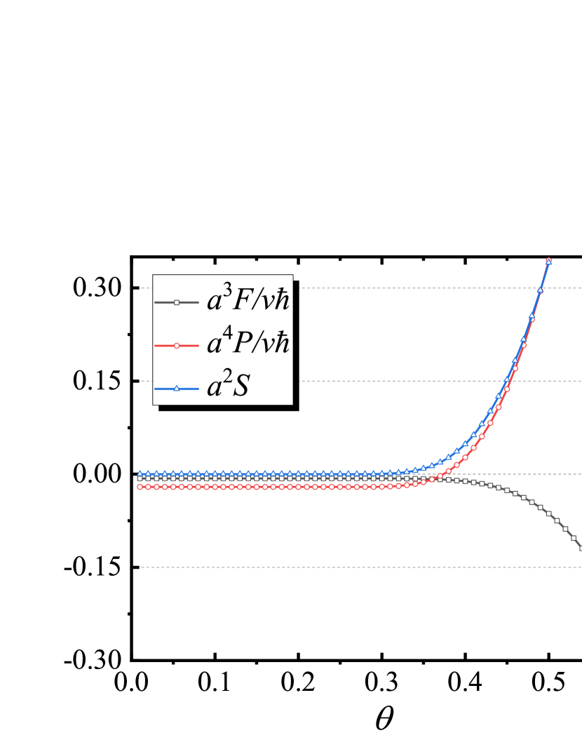
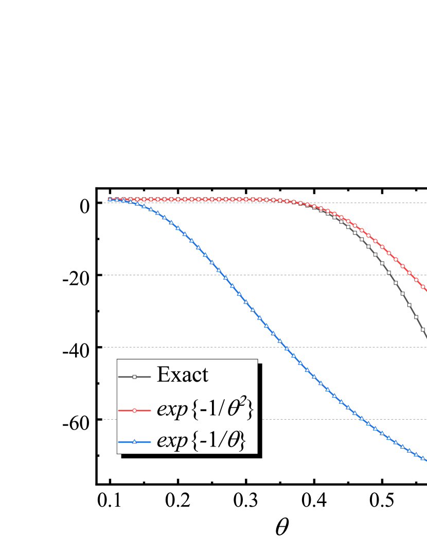
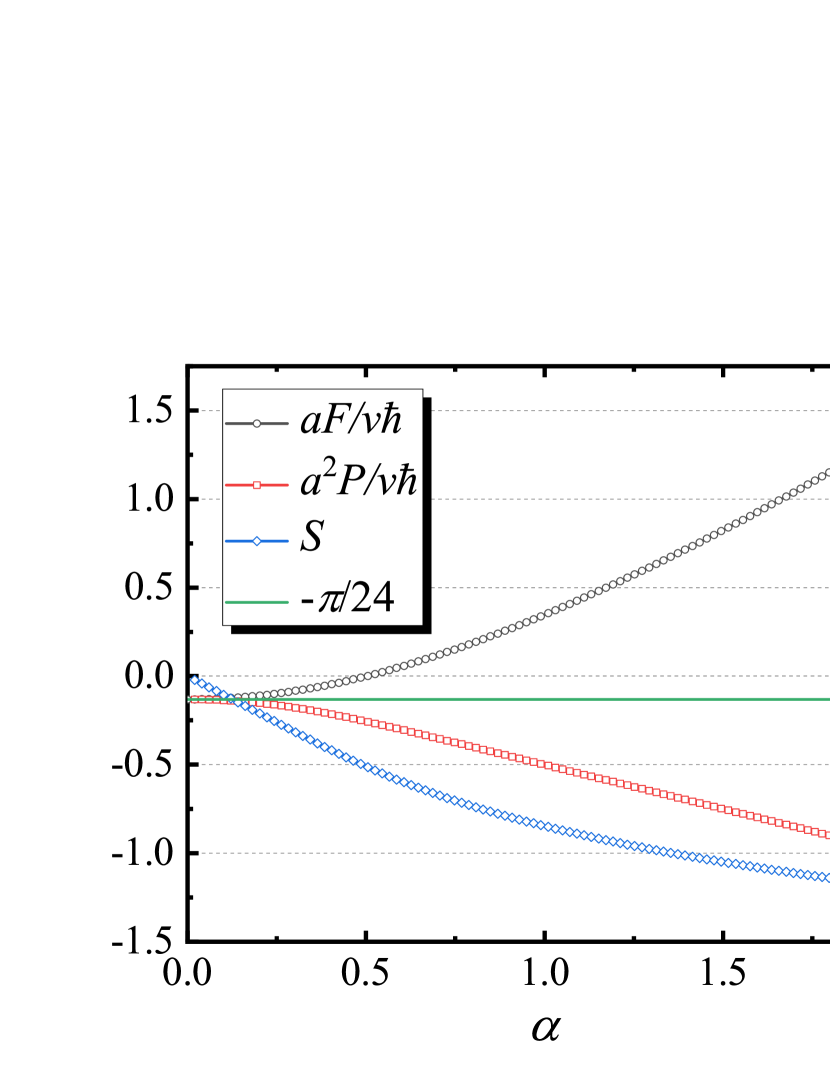
Fig. 6 shows the numerical results of Gibbs free energy, Casimir force and Casimir entropy. The results show similar character as the one-dimensional scalar field.

Now we analysis the asymptotic behavior at low temperature. In this case, we can use the definition of polylogarithm function,

$$\textrm{Li}_{3}(z)=\sum_{k=1}^{\infty}\frac{z^{k}}{k^{n}},$$

(54)

and keep only the leading order term, we get,

$$F=-\frac{{\pi^{2}}v\hbar}{1440a^{3}}\left[1+720\frac{aT}{\pi{v\hbar}}e^{-(\pi{v\hbar}/aT)^{2}}\right].$$

(55)

From this expression of Gibbs free energy, we can calculate the Casimir force,

$$P=-\frac{{\pi^{2}}v\hbar}{480a^{4}}+\left(\frac{\pi^{3}v^{2}\hbar^{2}}{a^{5}T}-\frac{\pi{T}}{a^{3}}\right)e^{-(\pi{v\hbar}/aT)^{2}},$$

(56)

and the Casimir entropy,

$$S=\frac{\pi}{2a^{2}}\left[2\left(\frac{\pi{v\hbar}}{aT}\right)^{2}+1\right]e^{-(\pi{v\hbar}/aT)^{2}}.$$

(57)

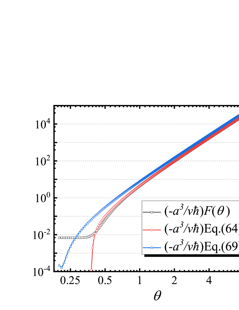
The exponential factor of Casimir force, $e^{-(\pi{v\hbar}/aT)^{2}}$, is different from the previous investigations (see e.g. Eq. (3.17) in [44] where the exponential factor is $e^{-\pi{v\hbar}/aT}$). We can get a similar result by using different approximations. From Eq. (50) and the definition of Casimir force, $P=-\partial{F}/\partial{a}$, we get the thermal correction of Casimir force,

$$\Delta{P}^{T}=\frac{\pi{T}}{2a^{3}}\sum_{l=1}^{\infty}l^{2}\int_{l\pi{v\hbar}/aT}^{\infty}\frac{1}{e^{y}-1}dy,$$

(58)

here we have defined the integration variable, $y=\sqrt{(v\hbar{k}/T)^{2}+(l\pi{v\hbar}/aT)^{2}}$. Completing the integration of $y$, we get,

$$\Delta{P}^{T}=-\frac{\pi{T}}{2a^{3}}\sum_{l=1}^{\infty}l^{2}\log\left(1-e^{-l\pi{v\hbar}/aT}\right).$$

(59)

In the low temperature limit, $T\rightarrow 0$, we keep the leading order term of $e^{-l\pi{v\hbar}/aT}$, and find,

$$P=-\frac{{\pi^{2}}v\hbar}{480a^{4}}+\Delta{P}^{T}=-\frac{{\pi^{2}}v\hbar}{480a^{4}}+\frac{\pi{T}}{2a^{3}}e^{-\pi{v\hbar}/aT}.$$

(60)

We get the low-temperature approximatin shown in Refs. [44, 45, 46, 47]. Fig. 5 shows a comparison of the two approximations, Eqs. (56) and (60). This result shows the $e^{-1/\theta^{2}}$ decay behavior of the thermal correction of Casimir force in the low temperature regime.

Now we analysis the asymptotic behavior at high temperature. In this case, $1/\theta$ is small, the summation can be approximated by integration, we use the Abel-Plana formula to estimate the summation,

	$$\displaystyle\sum_{l=1}^{\infty}\textrm{Li}_{3}\left[e^{-s\left(\frac{l}{\theta}\right)^{2}}\right]=\sum_{l=0}^{\infty}\textrm{Li}_{3}\left[e^{-s\left(\frac{l}{\theta}\right)^{2}}\right]-\zeta(3)$$
	$$\displaystyle\approx\left[\int_{0}^{\infty}\textrm{Li}_{3}(e^{-st^{2}/\theta^{2}})dt+\frac{1}{2}\zeta(3)\right]-\zeta(3),$$		(61)

here we have used $\textrm{Li}_{3}(1)=\zeta(3)$. Using the definition of polylogarithm function, Eq. (54), we can complete the integration,

$$\int_{0}^{\infty}\textrm{Li}_{3}(e^{-st^{2}/\theta^{2}})dt=\frac{\sqrt{\pi}\theta}{2\sqrt{s}}\sum_{k=1}^{\infty}k^{-7/2}=\frac{\sqrt{\pi}\theta}{2\sqrt{s}}\zeta\left(\frac{7}{2}\right),$$

(62)

Substituting these results into Eq. (51), we get,

$$F=-\frac{{\pi^{2}}v\hbar}{1440a^{3}}\left\{1+720\theta^{3}\left[\frac{3\sqrt{\pi}\theta}{4}\zeta\left(\frac{7}{2}\right)-\frac{1}{2}\zeta(3)\right]\right\},$$

(63)

Using the physical variables, we have,

$$F=-\frac{{\pi^{2}}v\hbar}{1440a^{3}}+\frac{\zeta(3)}{4\pi{v^{2}\hbar^{2}}}T^{3}-\frac{3\zeta(7/2)}{8\pi^{3/2}v^{3}\hbar^{3}}aT^{4}.$$

(64)

Note that, the term proportional to $aT^{4}$ is not the Gibbs free energy density of the free space in the regime $0<z<a$. The Gibbs free energy density of the free space in the regime $0<z<a$ equals to,

$$a\mathcal{F}_{\textrm{free}}=a\int\frac{d\bm{k}}{(2\pi)^{3}}\left[\frac{1}{\beta}\log\left(1-e^{-\beta{v\hbar}k}\right)\right]=-\frac{\pi^{2}{aT^{4}}}{90v^{3}\hbar^{3}}.$$

(65)

In previous investigations, there is another approximation which has been widely used. We show this approximation as follows. From Eq. (50), we can use $\log(1-x)=-\sum_{m=1}^{\infty}x^{m}/m$ in the high temperature regime to rewrite the thermal correction of free energy as,

$$\Delta{F}^{T}=-\frac{T}{4\pi}\sum_{l=1}^{\infty}\sum_{m=1}^{\infty}\int_{(l\pi/a)^{2}}^{\infty}\frac{e^{-mv\hbar\sqrt{u}/T}}{m}du,$$

(66)

Complete the integration, we get,

$$\Delta{F}^{T}=-\frac{T^{3}}{2\pi{v^{2}\hbar^{2}}}\sum_{l=1}^{\infty}\sum_{m=1}^{\infty}\frac{1}{m^{3}}\left(1+\frac{lm\pi{v\hbar}}{aT}\right)e^{-\frac{lm\pi{v\hbar}}{aT}},$$

(67)

Complete the summation over $l$, we get,

	$$\displaystyle\Delta{F}^{T}=-\frac{T^{3}}{4\pi{v^{2}\hbar^{2}}}\sum_{m=1}^{\infty}\frac{1}{m^{3}}\left[\coth\left(\frac{m\pi{v\hbar}}{2aT}\right)\right.$$
	$$\displaystyle\left.+\frac{m\pi{v\hbar}}{2aT}\textrm{csch}^{2}\left(\frac{m\pi{v\hbar}}{2aT}\right)\right]+\frac{\zeta(3)}{4\pi{v^{2}\hbar^{2}}}T^{3}.$$		(68)

Performing series expansion of $1/T$ and keep only the first term, we get,

$$F=-\frac{{\pi^{2}}v\hbar}{480a^{4}}+\Delta{F}^{T}=-\frac{{\pi^{2}}v\hbar}{480a^{4}}+\frac{\zeta(3)}{4\pi{v^{2}\hbar^{2}}}T^{3}-\frac{\pi^{2}{aT^{4}}}{90(v\hbar)^{3}}.$$

(69)

If we compare the analytical results and numerical result, one can find that there is a large difference.

Like the analysis of the one-dimensional scalar field, we may have two other proposals for the definition of Casimir free energy, by subtracting the term proportional $aT^{4}$ (proposal II, we consider the original proposal without any subtraction as proposal I), or subtracting the term proportional $aT^{4}$ and $T^{3}$ (the last two terms in Eq. (64), proposal III). For both these two new proposals, the Casimir entropy is negative in some regime.

In this work, we revisit the finite temperature Casimir effect for the one- and three-dimensional scalar field. For the one-dimensinal scalar field, we find that the low temperature approximation has a negative entropy problem in the regime $0<a<0.8T/v\hbar$, if we do not introduce any counter term for the thermal fluctuation. If we introduce the blackbody radiation energy as the counter term of thermal fluctuation (proposal II), or introduce another logarithmic divergence term as the counter term (proposal III), the entropy will be negative in the whole distance regime. For the three-dimensional scalar field, both the widely used low temperature approximation and high temperature approximation are deviated from the true limits. The leading order divergence term can not be canceled by the blackbody radiation energy. If we introduce the blackbody radiation energy, the leading order divergence term, or the leading order plus next leading order divergence terms as the counter terms, the entropy will be negative in some parameter regime. There results demonstrate that the blackbody radiation energy is not a proper counter term in the investigation of Casimir effect, other counter terms introduced in previous works need also to be modified.

The negative entropy problem has been investigated in previous works for different systems [48, 49, 50, 51]. Here, we find that, for the simplest situation, the scalar field with Dirichlet boundary condition, by using the most basic calculation method but with exact calculation result, the negative entropy problem exists for the widely used counter terms. These results reveal deeper issues in the thermal Casimir effect, and remind us to keep one eye on the counter terms used in the other advanced methods for the investigation of Casimir effect, e.g., the Lifshitz formula and quantum field theory approach. Our investigation can be generalized to the electromagnetic field straightforwardly. We advocate not introducing any counter terms for the thermal corrections of Casimir effect. If we choose this proposal (Proposal I), our theory predicts that the Casimir force is positive for $\theta=aT/\pi{c}{\hbar}{\gtrsim}0.374$, which gives $a{\gtrsim}9\mathrm{~{}{\mu}m}$ if we choose $T=300\textrm{~{}K}$ and $v$ equals to the speed of light in the vacuum. This is close to the limit that experiments can reach currently [52].

The authors are grateful for financial support from the National Natural Science Foundation of China (Grant No. 12174101) and the Fundamental Research Funds for the Central Universities (Grant No. 2022MS051).

References

- Casimir [1948] H. B. G. Casimir, On the attraction between two perfectly conducting plates, Proc. Kon. Nederland. Akad. Wetensch. , 793 (1948).
- Milonni [1994] P. W. Milonni, The Quantum Vacuum: An Introduction to Quantum Electrodynamics (Academic Press, San Diego, 1994).
- Bordag et al. [2001] M. Bordag, U. Mohideen, and V. M. Mostepanenko, New developments in the casimir effect, Physics Reports 353, 1 (2001).
- Bordag et al. [2009] M. Bordag, G. L. Klimchitskaya, U. Mohideen, and V. M. Mostepanenko, Advances in the Casimir Effect (Oxford University Press, Oxford, 2009).
- Klimchitskaya et al. [2009] G. L. Klimchitskaya, U. Mohideen, and V. M. Mostepanenko, The casimir force between real materials: Experiment and theory, Rev. Mod. Phys. 81, 1827 (2009).
- Munday et al. [2009] J. N. Munday, F. Capasso, and V. A. Parsegian, Measured long-range repulsive casimir-lifshitz forces, Nature 457, 170 (2009).
- Zhao et al. [2019] R. Zhao, L. Li, S. Yang, W. Bao, Y. Xia, P. D. Ashby, Y. Wang, and X. Zhang, Stable casimir equilibria and quantum trapping, Science 364, 984 (2019).
- Zhang et al. [2024] Y. Zhang, H. Zhang, X. Wang, Y. Wang, Y. Liu, S. Li, T. Zhang, C. Fan, and C. Zeng, Magnetic-field tuning of the Casimir force, Nat. Phys. 20, 1282 (2024).
- Hertlein et al. [2008] C. Hertlein, L. Helden, A. Gambassi, S. Dietrich, S. Dietrich, and C. Bechinger, Direct measurement of critical casimir forces, Nature 451, 172 (2008).
- Soyka et al. [2008] F. Soyka, O. Zvyagolskaya, C. Hertlein, L. Helden, and C. Bechinger, Critical casimir forces in colloidal suspensions on chemically patterned surfaces, Phys. Rev. Lett. 101, 208301 (2008).
- Bonn et al. [2009] D. Bonn, J. Otwinowski, S. Sacanna, H. Guo, G. Wegdam, and P. Schall, Direct observation of colloidal aggregation by critical casimir forces, Phys. Rev. Lett. 103, 156101 (2009).
- Nguyen et al. [2013] V. D. Nguyen, S. Faber, Z. Hu, G. H. Wegdam, and P. Schall, Controlling colloidal phase transitions with critical casimir forces, Nat. Commun. 4 (2013).
- Paladugu et al. [2016] S. Paladugu, A. Callegari, Y. Tuna, L. Barth, S. Dietrich, A. Gambassi, and G. Volpe, Nonadditivity of critical casimir forces, Nat. Commun. 7, 11403 (2016).
- Schmidt et al. [2022] F. Schmidt, A. Callegari, A. Daddi-Moussa-Ider, B. Munkhbat, R. Verre, T. Shegai, M. Käll, H. Löwen, A. Gambassi, and G. Volpe, Tunable critical casimir forces counteract casimir-lifshitz attraction, Nat. Phys. 10.1038/s41567-022-01795-6 (2022).
- Wilson et al. [2011] C. M. Wilson, G. Johansson, A. Pourkabirian, M. Simoen, J. R. Johansson, T. Duty, F. Nori, and P. Delsing, Observation of the dynamical casimir effect in a superconducting circuit, Nature 479, 376 (2011).
- Lähteenmäki et al. [2013] P. Lähteenmäki, G. S. Paraoanu, J. Hassel, and P. J. Hakonen, Dynamical casimir effect in a josephson metamaterial, Proc. Natl. Acad. Sci. U.S.A. 110, 4234 (2013).
- Felicetti et al. [2014] S. Felicetti, M. Sanz, L. Lamata, G. Romero, G. Johansson, P. Delsing, and E. Solano, Dynamical casimir effect entangles artificial atoms, Phys. Rev. Lett. 113, 093602 (2014).
- Vezzoli et al. [2018] S. Vezzoli, A. Mussot, N. Westerberg, A. Kudlinski, H. D. Saleh, A. Prain, F. Biancalana, É. Lantz, and D. Faccio, Optical analogue of the dynamical casimir effect in a dispersion-oscillating fibre, Commun. Phys. 2, 10.1038/s42005-019-0183-z (2018).
- Somers et al. [2018] D. A. T. Somers, J. L. Garrett, K. J. Palm, and J. N. Munday, Measurement of the casimir torque, Nature 564, 386 (2018).
- Levin et al. [2010] M. Levin, A. P. McCauley, A. W. Rodriguez, M. T. H. Reid, and S. G. Johnson, Casimir repulsion between metallic objects in vacuum, Phys. Rev. Lett. 105, 090403 (2010).
- Zhao et al. [2009] R. Zhao, J. Zhou, T. Koschny, E. N. Economou, and C. M. Soukoulis, Repulsive casimir force in chiral metamaterials, Phys. Rev. Lett. 103, 103602 (2009).
- Song et al. [2017] G. Song, J. Xu, C. Zhu, P. He, Y. Yang, and S.-Y. Zhu, Casimir force between hyperbolic metamaterials, Phys. Rev. A 95, 023814 (2017).
- Grushin and Cortijo [2011] A. G. Grushin and A. Cortijo, Tunable casimir repulsion with three-dimensional topological insulators, Phys. Rev. Lett. 106, 020403 (2011).
- Tse and MacDonald [2012] W.-K. Tse and A. H. MacDonald, Quantized casimir force, Phys. Rev. Lett. 109, 236806 (2012).
- Rodriguez-Lopez and Grushin [2014] P. Rodriguez-Lopez and A. G. Grushin, Repulsive casimir effect with chern insulators, Phys. Rev. Lett. 112, 056804 (2014).
- Wilson et al. [2015] J. H. Wilson, A. A. Allocca, and V. Galitski, Repulsive casimir force between weyl semimetals, Phys. Rev. B 91, 235115 (2015).
- Jiang and Wilczek [2019] Q.-D. Jiang and F. Wilczek, Chiral casimir forces: Repulsive, enhanced, tunable, Phys. Rev. B 99, 125403 (2019).
- Quach [2015] J. Q. Quach, Gravitational casimir effect, Phys. Rev. Lett. 114, 081104 (2015).
- Bellucci and Saharian [2009] S. Bellucci and A. A. Saharian, Fermionic casimir effect for parallel plates in the presence of compact dimensions with applications to nanotubes, Phys. Rev. D 80, 105003 (2009).
- Costantino and Fichet [2020] A. Costantino and S. Fichet, The neutrino casimir force, J. High Energy Phys. 2020 (9), 122.
- Schecter and Kamenev [2014] M. Schecter and A. Kamenev, Phonon-mediated casimir interaction between mobile impurities in one-dimensional quantum liquids, Phys. Rev. Lett. 112, 155301 (2014).
- Nakata and Suzuki [2023] K. Nakata and K. Suzuki, Magnonic casimir effect in ferrimagnets, Phys. Rev. Lett. 130, 096702 (2023).
- Mostepanenko [2021] V. M. Mostepanenko, Casimir puzzle and casimir conundrum: Discovery and search for resolution, Universe 7, 10.3390/universe7040084 (2021).
- Mostepanenko et al. [2006] V. M. Mostepanenko, V. B. Bezerra, R. S. Decca, B. Geyer, E. Fischbach, G. L. Klimchitskaya, D. E. Krause, D. López, and C. Romero, Present status of controversies regarding the thermal casimir force, J. Phys. A Math. Gen. 39, 6589 (2006).
- Mostepanenko and Geyer [2008] V. M. Mostepanenko and B. Geyer, New approach to the thermal casimir force between real metals, J. PHYS. A-MATH. THEOR. 41, 164014 (2008).
- Klimchitskaya and Geyer [2008] G. L. Klimchitskaya and B. Geyer, Problems in the theory of the thermal casimir force between dielectrics and semiconductors, J. PHYS. A-MATH. THEOR. 41, 164032 (2008).
- Lamoreaux [2012] S. K. Lamoreaux, The casimir force and related effects: The status of the finite temperature correction and limits on new long-range forces, Annu. Rev. Nucl. Part. S. 62, 37 (2012).
- Hartmann et al. [2017] M. Hartmann, G.-L. Ingold, and P. A. M. Neto, Plasma versus drude modeling of the casimir force: Beyond the proximity force approximation, Phys. Rev. Lett. 119, 043901 (2017).
- Liu et al. [2019] M. Liu, J. Xu, G. L. Klimchitskaya, V. M. Mostepanenko, and U. Mohideen, Examining the casimir puzzle with an upgraded afm-based technique and advanced surface cleaning, Phys. Rev. B 100, 081406 (2019).
- Klimchitskaya and Mostepanenko [2022] G. L. Klimchitskaya and V. M. Mostepanenko, Current status of the problem of thermal casimir force, INT. J. MOD. PHYS. A 37, 2241002 (2022).
- Bezerra et al. [2004] V. B. Bezerra, G. L. Klimchitskaya, V. M. Mostepanenko, and C. Romero, Violation of the nernst heat theorem in the theory of the thermal casimir force between drude metals, Phys. Rev. A 69, 022119 (2004).
- Polchinski [1998] J. Polchinski, String Theory (Cambridge University Press, 1998).
- Green et al. [1987] M. Green, J. Schwartz, and E. Witten, Superstring Theory (Cambridge University Press, 1987).
- Schwinger et al. [1978] J. Schwinger, L. L. DeRaad, and K. A. Milton, Casimir effect in dielectrics, Ann. Phys. 115, 1 (1978).
- Mehra [1967] J. Mehra, Temperature correction to the casimir effect, Physica 37, 145 (1967).
- Geyer et al. [2008] B. Geyer, G. L. Klimchitskaya, and V. M. Mostepanenko, Thermal casimir effect in ideal metal rectangular boxes, EUR. PHYS. J. C 57, 823 (2008).
- Zhang [2017] A. Zhang, Theoretical analysis of casimir and thermal casimir effect in stationary space-time, Phys. Lett. B 773, 125 (2017).
- Milton et al. [2017] K. A. Milton, P. Kalauni, P. Parashar, and Y. Li, Casimir self-entropy of a spherical electromagnetic -function shell, Phys. Rev. D 96, 085007 (2017).
- Bordag [2018] M. Bordag, Free energy and entropy for thin sheets, Phys. Rev. D 98, 085010 (2018).
- Milton et al. [2019] K. A. Milton, P. Kalauni, P. Parashar, and Y. Li, Remarks on the casimir self-entropy of a spherical electromagnetic -function shell, Phys. Rev. D 99, 045013 (2019).
- Li et al. [2021] Y. Li, K. A. Milton, P. Parashar, and L. Hong, Negativity of the casimir self-entropy in spherical geometries, Entropy 23 (2021).
- Sushkov et al. [2011] A. O. Sushkov, W. J. Kim, D. A. R. Dalvit, and S. K. Lamoreaux, Observation of the thermal Casimir force, Nat. Phys. 7, 230 (2011).