First passage properties of asymmetric Lévy flights

Amin Padash^†,♯, Aleksei V. Chechkin^♯,‡, Bartlomiej Dybiec^♭, Ilya Pavlyukevich^§, Babak Shokri^†,¶, & Ralf Metzler^♯ ^† Physics Department of Shahid Beheshti University, 19839-69411 Tehran, Iran
^♯ Institute for Physics & Astronomy, University of Potsdam, 14476 Potsdam-Golm, Germany
^‡ Akhiezer Institute for Theoretical Physics, 61108 Kharkov, Ukraine
^♭ Marian Smoluchowski Institute of Physics and Mark Kac Center for Complex Systems Research, Jagiellonian University, ul. St. Lojasiewicza 11, 30-348 Krakow, Poland
^§ Friedrich Schiller University Jena, Faculty of Mathematics and Computer Science, Institute for Mathematics, 07737 Jena, Germany
^¶ Laser and Plasma Research Institute, Shahid Beheshti University, 19839-69411 Tehran, Iran rmetzler@uni-potsdam.de (Corresponding author)

Abstract

Lévy Flights are paradigmatic generalised random walk processes, in which the independent stationary increments—the "jump lengths"—are drawn from an $\alpha$ -stable jump length distribution with long-tailed, power-law asymptote. As a result, the variance of Lévy Flights diverges and the trajectory is characterised by occasional extremely long jumps. Such long jumps significantly decrease the probability to revisit previous points of visitation, rendering Lévy Flights efficient search processes in one and two dimensions. To further quantify their precise property as random search strategies we here study the first-passage time properties of Lévy Flights in one-dimensional semi-infinite and bounded domains for symmetric and asymmetric jump length distributions. To obtain the full probability density function of first-passage times for these cases we employ two complementary methods. One approach is based on the space-fractional diffusion equation for the probability density function, from which the survival probability is obtained for different values of the stable index $\alpha$ and the skewness (asymmetry) parameter $\beta$ . The other approach is based on the stochastic Langevin equation with $\alpha$ -stable driving noise. Both methods have their advantages and disadvantages for explicit calculations and numerical evaluation, and the complementary approach involving both methods will be profitable for concrete applications. We also make use of the Skorokhod theorem for processes with independent increments and demonstrate that the numerical results are in good agreement with the analytical expressions for the probability density function of the first-passage times.

1 Introduction

Normal Brownian motion described by Fick’s second law, the diffusion equation, is characterised by the linear time dependence $\langle x^{2}(t)\rangle\simeq t$ of the mean squared displacement (MSD) [1]. Deviations from this Fickean time dependence typically occur in the power-law form $\langle x^{2}(t)\rangle\simeq t^{\kappa}$ of the MSD [2, 3]. Depending on the value of the anomalous diffusion exponent $\kappa$ we distinguish between subdiffusion for $0<\kappa<1$ , normal, Fickean diffusion for $\kappa=1$ , superdiffusion for $1<\kappa<2$ , and ballistic, wave-like motion for $\kappa=2$ . The range $\kappa>2$ is sometimes referred to as hyperdiffusion. The theoretical description of anomalous diffusion phenomena of physical particles (passive or active) often requires a radical departure from the classical formalism for Brownian motion. Namely, effects of energetic or spatial disorder, collective dynamics, or non-equilibrium conditions need to be addressed with more complex approaches [2, 4]. For instance, fractional Brownian motion [5] is a process in which the Langevin equation is driven by Gaussian yet power-law correlated noise (fractional Gaussian noise) effecting both sub- and superdiffusion. The generalised Langevin equation [6] includes a memory integral with a kernel, that balances the input fractional Gaussian noise and effects a thermalised process. Processes with explicitly time or position dependent diffusion coefficients such as scaled Brownian motion [7] or heterogeneous diffusion processes [8], respectively, also lead to sub- and superdiffusion. Diffusion on fractals [9] due to the fact that the particle in the highly ramified environment often has to back-track its motion, has similar characteristics as subdiffusive fractional Brownian motion. We finally mention the continuous time random walk model, in which the standard Pearson walk was generalised to include continuous waiting times [10]. When the distribution of waiting times becomes scale-free, with diverging characteristic waiting time, the continuous time random walk process is subdiffusive [11, 12]. Conversely, when the continuous time random walk has a finite characteristic waiting time but is equipped with a scale-free distribution of jump lengths with power-law asymptote $\lambda(x)\sim|x|^{-1-\alpha}$ ( $0<\alpha<2$ ) the resulting process is a "Lévy flight" (LF). As in this case the variance of the process diverges, diffusion can be characterised in terms of rescaled fractional order moments ${\langle|x(t)|^{\eta}\rangle}^{2/\eta}\simeq t^{2/\alpha}$ with $0<\eta<\alpha$ [3, 13, 14, 15, 16, 17]. Mathematically, asymptotic power-law forms of the jump length distribution can be explained by the generalised central limit theorem [2, 18, 19, 20], which gives rise to the much higher likelihood for extremely long jumps [21, 22, 23] in comparison to conventional Pearson random walks.

Lévy stable laws play a crucial role in the statistical description of scale invariant stochastic processes [21, 24] not only in physical contexts but also in biological, chemical, geophysical, sociological, economical or financial systems, among others. In physics Lévy statistics were demonstrated to explain deviations of complex systems from the Gaussian paradigm, inter alia, for the power-law blinking of nano-scale light emitters [25], diffusive transport of light [26], photons in hot atomic vapours [27], tracer particles in a rotating flow [28], passive scalars in vortices in shear [29], anomalous diffusion in disordered media [2], weakly chaotic and Hamiltonian systems [30, 31], in the divergence of kinetic energy fluctuations of a single ion in an optical lattice [32], fluctuations in the transition energy of a single molecule embedded in a solid [33], in the interaction of two level systems with single molecules [34], the distribution of random single molecule line shapes in low temperature glasses [35], the diffusion of a collection of ultra-cold atoms and single ions in optical lattices [36], but also in reaction diffusion systems [37, 38]. Lévy statistics was observed experimentally in tokamak and stellarator fusion devices [39, 40, 41]. It was also shown that the phenomenon of L-H transitions observed in the stellarator is accompanied by the crossover from Lévy to Gaussian fluctuation statistics [42]. Numerous examples for Lévy statistics exist in the dynamics of plasmas, including the anomalous transport in magnetic confinement [43, 44, 45, 46, 47], the dynamics of a charged particle in a plasma [48, 49], anomalous transport of ions and electrons in solar winds [50], nonlocal transport in plasma turbulence [51, 52, 53, 54, 55], and heat transport in magnetised plasmas [56, 57].

In the biological sciences, many organisms from bacteria to humans use Lévy stable relocation statistics in their search for resources [58], tracer motion in living cells [59, 60, 61, 62], or the superdiffusive motion of bacteria within a swarm [63]. On long, fast-folding polymers the search process of a binding molecule is based on Lévy motion [64, 65, 66, 67]. In geoscience paleoclimate time series show signatures of Lévy noise [68], earthquake statistics exhibit distinct power-law behaviour [69], as well as tracer plumes in heterogeneous aquifers [70, 71, 72], and the transport of ensembles of particles on the Earth surface [73]. The mechanisms of the worldwide spread of infectious diseases [74], pollen dispersal by bees [75] and human mobility patterns and social interactions revealed by tracing mobile phones or following banknotes [76, 77, 78, 79, 80, 81] also reveal Lévy statistics. Evidence of Lévy stable laws was also unveiled in the human cognition for the retrieval dynamics of memory [82] and in human mental search [83, 84, 85], as well as search in multiplex networks [86]. The optimal search patterns of robots were shown to be based on Lévy stable laws [87]. In finance and economical contexts [88, 89, 90, 91] Lévy statistics govern the distribution of trades. A particular area in which Lévy relocation statistics has been widely explored is movement ecology [92]. Search patterns of foraging animals [93] that follow Lévy statistics include marine predators [94, 95], albatross birds [96], Agrotis segetum moths [97], fruit flies (Drosophila melanogaster) [98], bumblebees [99], jellyfish [100], goats [101, 102], immune function of human T cells [103] and human hunter-gatherers [104]. We hasten to note that in the context of animal movement there exist some debates on the predominance of Lévy search patterns, especially the disqualification of Lévy statistics for albatrosses [105, 106] in [107] became a strong argument against the LF hypothesis. However, there is strong evidence that for individual albatross birds LFs are indeed a real search pattern [108]. Moreover, [109] reported that for spider monkeys the foraging pattern is deterministic, mussel movements are rather multimodal [110, 111] and black bean aphids individually move in a predominantly diffusive manner [112].

The efficiency of search processes is typically benchmarked by the time it takes the searcher to reach a certain region in space. One relevant measure is therefore the first-passage time, quantifying the time it takes from the original position to first cross a point located at a given distance away. For instance, the first-passage time in a financial time series could be defined by a preset increase or decrease in the price of a given stock. Once this threshold value is reached, the stock is sold or bought. Similarly, we could talk about the instant of time when foraging animals first randomly locate a resource-rich area away from their original location. Such first-passage times in a stochastic search process will vary from realisation to realisation, and can be quantified by the first-passage time density $\wp(t)$ . While the mean first-passage time $\langle t\rangle=\int_{0}^{\infty}t\wp(t)dt$ can capture some aspects of this dynamics,¹¹1Often, a better choice is the mean inverse first-passage time $\langle 1/t\rangle$ [113]. the full information encoded in $\wp(t)$ provides significant additional insight [114, 115, 116]. Here we study the first-passage properties for a general class of $\alpha$ -stable Lévy laws. We go beyond previous approaches [113, 117, 118, 119, 120, 121, 122, 123, 124, 125, 126, 127, 128] focusing on symmetric and one-sided $\alpha$ -stable relocation distributions and consider $\alpha$ -stable laws with arbitrary asymmetry in semi-infinite and bounded domains. Our approach is based on the convenient formulation of LFs in terms of the space-fractional diffusion equation. We derive these integro-differential equations for LFs based on general asymmetric $\alpha$ -stable distributions of relocation lengths in finite domains, and thus go beyond studies of the exit time and escape probability in bounded domain for symmetric LFs [129, 130, 131]. An important aspect of this study is that we complement our results with numerical analyses of the (stochastic) Langevin equation for LFs and show how both approaches complement each other.

The paper is organised as follows. In section 2 we define Lévy stable laws and the associated fractional diffusion equation. In section 3 we set up our numerical model for the fractional diffusion equation and the associated Langevin equation. Moreover, a comparison between the numerical method and $\alpha$ -stable distributions for symmetric and asymmetric density functions is presented. Section 4 then presents the numerical results for the survival probability and first-passage time density for both symmetric and asymmetric probability density functions. Our findings are compared with results derived from the Skorokhod theorem for symmetric, one-sided, and extremal two-sided stable distributions. We draw our conclusion in section 5. In the Appendices, we present details of several derivations.

2 $\alpha$ -stable processes and space-fractional diffusion equations

An $\alpha$ -stable Lévy process $X(t)$ with $X(0)=0$ and probability density function (PDF) $\ell_{\alpha,\beta}(x,t)$ is fully specified by its characteristic function in the Fourier domain as [18, 132]

	$\displaystyle\hat{\ell}_{\alpha,\beta}(k,t)$	$\displaystyle=$	$\displaystyle\int\limits_{-\infty}^{\infty}\ell_{\alpha,\beta}(x,t)\exp(\mathrm{i}kx)\mathrm{d}x$		(1)
		$\displaystyle=$	$\displaystyle\exp(-tK_{\alpha}\|k\|^{\alpha}[1-\mathrm{i}\beta\mathrm{sgn}(k)\omega(k,\alpha)]+\mathrm{i}\mu kt),$		(1)

where the index $\alpha$ with $0<\alpha\leq 2$ is called the index of stability or Lévy index, and the skewness parameter $\beta$ is allowed to vary within the limits $-1\leq\beta\leq 1$ . Further, the generalised diffusion coefficient $K_{\alpha}>0$ is a scale parameter, the shift parameter $\mu$ is any real number, and the phase factor $\omega$ is defined as

\omega(k,\alpha)=\left\{\begin{array}[]{lr}\tan(\frac{\pi\alpha}{2}),&\alpha\neq 1\\ -\frac{2}{\pi}\ln|k|,&\alpha=1\end{array}\right..

(2)

In the real space-time domain the PDF of the $\alpha$ -stable distribution can be expressed via elementary functions for the following three cases:

(a) Gaussian distribution, $\alpha=2$ , $\beta$ irrelevant:

\ell_{2}(x,t)=\frac{1}{\sqrt{4\pi K_{2}t}}\exp\left(-\frac{(x-\mu t)^{2}}{4K_{2}t}\right),\qquad-\infty<x<\infty.

(3a)

(b) Cauchy distribution, $\alpha=1$ , $\beta=0$ :

\ell_{1,0}(x,t)=\frac{1}{\pi}\frac{K_{1}t}{(x-\mu t)^{2}+(K_{1}t)^{2}},\qquad-\infty<x<\infty.

(3b)

In physics, the Cauchy distribution is also often called a Lorentz distribution.

\ell_{1/2,1}(x,t)=\frac{K_{1/2}t}{\sqrt{2\pi(x-\mu t)^{3}}}\exp\left(-\frac{(K_{1/2}t)^{2}}{2(x-\mu t)}\right),\qquad x\geq 0.

(3c)

Schneider reported the representation of general Lévy stable densities in terms of Fox $H$ -functions [133, 134, 135]. Somewhat simpler representations for rational indices $\alpha$ and $\beta$ are given in [136, 137]. More information on Lévy stable densities and their parametrisation are provided in A.

Physically, the parameter $\mu$ accounts for a constant drift in the system. In this paper we consider the first-passage process in the absence of a drift, thus in what follows we set $\mu=0$ . Let us first consider the case $\alpha\neq 1$ and $-1\leq\beta\leq 1$ . The corresponding space-fractional diffusion equation for the PDF $\ell_{\alpha,\beta}(x,t)$ then reads

\frac{\partial\ell_{\alpha,\beta}(x,t)}{\partial t}=K_{\alpha}\,D^{\alpha}_{x}\ell_{\alpha,\beta}(x,t),\quad\ell_{\alpha,\beta}(x,0)=\delta(x),

(3d)

where $D_{x}^{\alpha}$ is the space-fractional derivative operator,

D^{\alpha}_{x}\ell_{\alpha,\beta}(x,t)=L_{\alpha,\beta}\,{}_{-\infty}D_{x}^{\alpha}\ell_{\alpha,\beta}(x,t)+R_{\alpha,\beta}\,{}_{x}D_{\infty}^{\alpha}\ell_{\alpha,\beta}(x,t),

(3e)

that we compose of ${}_{-\infty}D_{x}^{\alpha}$ and ${}_{x}D_{\infty}^{\alpha}$ , the left and right hand side space-fractional operators, respectively. We use the Caputo form of the operators defined by $(n-1<\alpha<n)$ [138]


${}_{-\infty}D_{x}^{\alpha}f(x)$	$\displaystyle=$	$\displaystyle\frac{1}{\Gamma(n-\alpha)}\int\limits_{-\infty}^{x}\frac{f^{(n)}(\zeta)}{(x-\zeta)^{\alpha-n+1}}\,\mathrm{d}\zeta$	(3fa)
${}_{x}D_{\infty}^{\alpha}f(x)$	$\displaystyle=$	$\displaystyle\frac{(-1)^{n}}{\Gamma(n-\alpha)}\int\limits_{x}^{\infty}\frac{f^{(n)}(\zeta)}{(\zeta-x)^{\alpha-n+1}}\,\mathrm{d}\zeta$	(3fb)

and $L_{\alpha,\beta}$ and $R_{\alpha,\beta}$ are the left and right weight coefficients, defined as [52, 53]

L_{\alpha,\beta}=-\frac{1+\beta}{2\cos(\frac{\alpha\pi}{2})},\qquad R_{\alpha,\beta}=-\frac{1-\beta}{2\cos(\frac{\alpha\pi}{2})}.

(3fg)

The Fourier transforms of the operators (3fa) and (3fb) have the forms [138]


	${}_{-\infty}D_{x}^{\alpha}f(x)\div(-\mathrm{i}k)^{\alpha}\hat{f}(k)=\|k\|^{\alpha}\exp\left({-\frac{\alpha\pi\mathrm{i}}{2}\mathrm{sgn}(k)}\right)\hat{f}(k),$		(3fha)
	${}_{x}D_{\infty}^{\alpha}f(x)\div(\mathrm{i}k)^{\alpha}\hat{f}(k)=\|k\|^{\alpha}\exp\left({\frac{\alpha\pi\mathrm{i}}{2}\mathrm{sgn}(k)}\right)\hat{f}(k),$		(3fhb)

where $\div$ defines the Fourier transform pairs.

For the case $\alpha=1$ and $\beta=0$ we have $L_{1,0}=R_{1,0}=1/\pi$ [139], and instead of equation (3e) we find

\frac{\partial\ell_{1,0}(x,t)}{\partial t}=-K_{\alpha}\frac{\partial}{\partial x}\mathscr{H}\Big{\{}\ell_{1,0}(x,t)\Big{\}},

(3fhi)

where $\mathscr{H}$ is the Hilbert transform

\mathscr{H}\Big{\{}f(x)\Big{\}}=\frac{1}{\pi}\mathchoice{{\vbox{\hbox{$\textstyle-$}}\kern-5.34723pt}}{{\vbox{\hbox{$\scriptstyle-$}}\kern-3.77364pt}}{{\vbox{\hbox{$\scriptscriptstyle-$}}\kern-3.19882pt}}{{\vbox{\hbox{$\scriptscriptstyle-$}}\kern-3.03651pt}}\!\int\limits_{-\infty}^{\infty}\frac{f(\zeta)}{x-\zeta}\mathrm{d}\zeta,

(3fhj)

in terms of the principle value integral $\mathchoice{{\vbox{\hbox{$\textstyle-$}}\kern-5.34723pt}}{{\vbox{\hbox{$\scriptstyle-$}}\kern-3.77364pt}}{{\vbox{\hbox{$\scriptscriptstyle-$}}\kern-3.19882pt}}{{\vbox{\hbox{$\scriptscriptstyle-$}}\kern-3.03651pt}}\!\int$ . In Fourier space the Hilbert transform has the simple form

\mathscr{H}\Big{\{}f(x)\Big{\}}\div\mathrm{i}\mathrm{sgn}(k)\hat{f}(k).

(3fhk)

In what follows we do not consider the particular case $\alpha=1$ , $\beta\neq 0$ since it cannot be described in terms of a space-fractional operator. For all other choices of the parameters by substitution of relations (3fha), (3fhb), and (3fhk) into equation (3d) we recover the characteristic function (1) of the $\alpha$ -stable process after Fourier transform.

3 Numerical scheme

To determine the first-passage properties of $\alpha$ -stable processes we will employ different numerical schemes based on the space-fractional diffusion equation and the Langevin equation for LFs. We here detail their implementation.

3.1 Diffusion description

There are several numerical methods to solve space-fractional diffusion equations, such as the finite difference [140, 141] and finite element [142, 143, 144] methods as well as the spectral method [145, 146]. In this paper we use the finite difference method that uses differential quotients to replace the derivatives in the differential equations. The domain is partitioned in space and time, and approximations of the solution are computed. Due to causality we use forward differences in time on the left hand side of equation (3d),

\frac{\partial}{\partial t}f(x_{i},t_{j})\approx\frac{f^{j+1}_{i}-f^{j}_{i}}{\Delta t},

(3fhl)

where $f^{j}_{i}=f(x_{i},t_{j})$ , $x_{i}=(i-I/2)\Delta x$ , and $t_{j}=j\Delta t$ , where $\Delta x$ and $\Delta t$ are step sizes in position and time, respectively. The $i$ and $j$ are non-negative integers, $i=0,1,2,\ldots,I$ , and further $x_{0}=-L$ , $x_{I}=L$ , and $\Delta x=2L/I$ . Similarly, $j=0,1,2,\ldots,J-1$ , $t_{0}=0$ , $t_{J}=t$ , and $\Delta t=t/J$ . Absorbing boundary conditions for the determination of the first-passage event imply $f_{0}^{j}=f_{I}^{j}=0$ for all $j$ . The integrals on the right hand side of equation (3d) are discretised as follows. For $0<\alpha<1$ ,

	$\int\limits_{-L}^{x_{i}}\frac{f^{(1)}(\zeta,t_{j})}{(x_{i}-\zeta)^{\alpha}}\mathrm{d}\zeta\approx\displaystyle\sum_{k=1}^{i}\frac{f^{j}_{k}-f^{j}_{k-1}}{\Delta x}\int\limits_{x_{k-1}}^{x_{k}}\frac{1}{(x_{i}-\zeta)^{\alpha}}\mathrm{d}\zeta,$	(3fhma)
for the left side derivative, and
	$\int\limits_{x_{i}}^{L}\frac{f^{(1)}(\zeta,t_{j})}{(\zeta-x_{i})^{\alpha}}\mathrm{d}\zeta\approx\displaystyle\sum_{k=i}^{I-1}\frac{f^{j}_{k+1}-f^{j}_{k}}{\Delta x}\int\limits_{x_{k}}^{x_{k+1}}\frac{1}{(\zeta-x_{i})^{\alpha}}\mathrm{d}\zeta,$	(3fhmb)

for the right side derivative. Thus the idea is to approximate only the derivative by the differences. The integral kernel is then calculated explicitly. For the estimation of the error in this scheme we refer to C. For the case $1<\alpha<2$ we use the central difference approximation, namely,

	$\int\limits_{-L}^{x_{i}}\frac{f^{(2)}(\zeta,t_{j})}{(x_{i}-\zeta)^{\alpha-1}}\mathrm{d}\zeta\approx\displaystyle\sum_{k=1}^{i}\frac{f^{j}_{k+1}-2f^{j}_{k}+f^{j}_{k-1}}{(\Delta x)^{2}}\int\limits_{x_{k-1}}^{x_{k}}\frac{1}{(x_{i}-\zeta)^{\alpha-1}}\mathrm{d}\zeta,$	(3fhmna)
for the left side, and
	$\int\limits_{x_{i}}^{L}\frac{f^{(2)}(\zeta,t_{j})}{(\zeta-x_{i})^{\alpha-1}}\mathrm{d}\zeta\approx\displaystyle\sum_{k=i}^{I-1}\frac{f^{j}_{k+1}-2f^{j}_{k}+f^{j}_{k-1}}{(\Delta x)^{2}}\int\limits_{x_{k}}^{x_{k+1}}\frac{1}{(\zeta-x_{i})^{\alpha-1}}\mathrm{d}\zeta,$	(3fhmnb)

for the right side. For the special case $\alpha=1$ , $\beta=0$ by using the discrete Hilbert transform [147] we approximate the derivative in space, namely

-\frac{d}{dx}(\mathscr{H}\left\{f(x,t)\right\})\approx-\frac{2}{\pi}\displaystyle\sum_{k=1}^{i}\frac{f^{j}_{k}-f^{j}_{k-1}}{\Delta x}\frac{1}{2(i-k)+1}-\frac{2}{\pi}\displaystyle\sum_{k=i}^{I-1}\frac{f^{j}_{k}-f^{j}_{k+1}}{\Delta x}\frac{1}{2(k-i)+1}.

(3fhmno)

For further details of the numerical scheme we refer the reader to B. To improve the stability we use the Crank-Nicolson method. By substitution of equations (3fhl) to (3fhmno) into equation (3d) we obtain

\mathbf{A}f^{j+1}=\mathbf{B}f^{j},

(3fhmnp)

in which the coefficients $\mathbf{A}$ and $\mathbf{B}$ have matrix form with dimension $(I+1)\times(I+1)$ and $j=0,1,2,\ldots,J-1$ . In the numerical scheme the initial condition $f(x,0)=\delta(x)$ is approximated as

	$f(x_{i},t_{0})=\left\{\begin{array}[]{ll}\frac{1}{\Delta x},&i=L/\Delta x\\ 0,&\mbox{otherwise}\end{array}\right..$	(3fhmnqa)
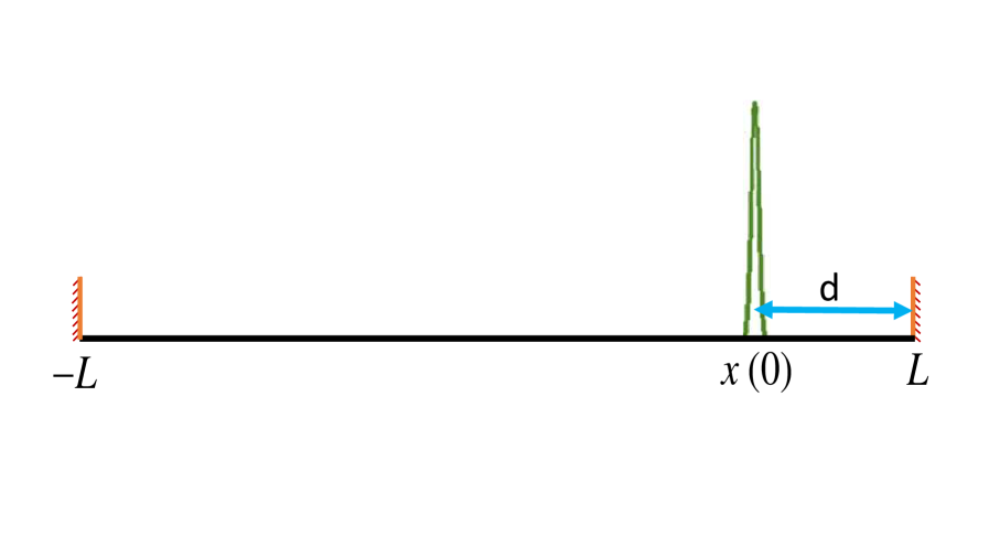
For the setup used in our numerical simulations, see section 4 below, the initial point is $f(x,0)=\delta(x-x(0))$ at $x(0)=L-d$ , where $d<2L$ is the distance of $x(0)$ from the right interval boundary (see figure 3). For this case we implement the initial condition as
	$f(x_{i},t_{0})=\left\{\begin{array}[]{ll}\frac{1}{\Delta x},&i=(2L-d)/\Delta x\\ 0,&\mbox{otherwise}\end{array}\right..$	(3fhmnqb)

In the next step the time evolution of the PDF is obtained by using the absorbing boundary conditions $f_{0}^{j}=f_{I}^{j}=0$ for all $j$ and applying to the matrix coefficients $\mathbf{A}$ and $\mathbf{B}$ .

3.2 Langevin dynamics

The fractional diffusion equation (3d) can be related to the Langevin equation [14, 123, 148]

\frac{\mathrm{d}}{\mathrm{d}t}{x}(t)=K_{\alpha}^{1/\alpha}\zeta(t),

(3fhmnqr)

where $\zeta(t)$ is white Lévy noise characterised by the same $\alpha$ and $\beta$ parameters as the space-fractional operator (3e) and with unit scale parameter. The Langevin equation (3fhmnqr) provides a microscopic (trajectory-wise) representation of the space-fractional diffusion equation (3d). Therefore, from an ensemble of trajectories generated from equation (3fhmnqr) it is possible to estimate the time dependent PDF whose evolution is described by equation (3d). In numerical simulations Lévy flights can be described by the discretised form of the Langevin equation

x(t+\Delta t)=x(t)+K_{\alpha}^{1/\alpha}(\Delta t)^{1/\alpha}\zeta,

(3fhmnqs)

where $\zeta$ stands for the $\alpha$ -stable random variable with a unit scale parameter [18, 149] and the same index of stability $\alpha$ and skewness $\beta$ parameters as in equation (3fhmnqr). Relation (3fhmnqs) is exactly the Euler-Maruyama approximation [150, 151, 152] to the general $\alpha$ -stable Lévy process. From the trajectories $x(t)$ , see equations (3fhmnqr) and (3fhmnqs), it is also possible to estimate the first-passage time $\tau$ as

\tau=\min\{t:|x(t)|\geq L\}.

(3fhmnqt)

From the ensemble of first-passage times it is also possible to estimate the survival probability $S(t)$ , the complementary cumulative density of first-passage times. More precisely, the initial condition is $S(0)=1$ , and at every recorded first-passage event at time $\tau_{i}$ , $S(t)$ is decreased by the amount $1/N$ , where $N$ is the number of records of first-passage times. If a given estimation of the first-passage time is recorded $k$ times the survival probability is decreased by $k/N$ . For a finite set of first-passage times there exists a small fraction of very large first-passage times. Therefore, this estimation becomes poorer with increasing time $t$ . In the next section we present a comparison between the numerical solution of equation (3d) and the $\alpha$ -stable probability laws with characteristic function (1).

3.3 Comparison with $\alpha$ -stable distributions

We now show that the difference scheme for the space-fractional diffusion equation provides excellent agreement with the theoretical results for the shapes of $\alpha$ -stable probability densities. To this end we use a MATLAB code to obtain the inverse Fourier transform of the characteristic function [153]. This programme employs Zolotarev’s so-called M-form for the parametrisation of $\alpha$ -stable distributions with parameters $\alpha$ , $\beta_{M}$ , $\mu_{M}$ , and $K_{\alpha}^{M}$ , while in the main text we use the A-form with parameters $\alpha$ , $\beta_{A}$ , $\mu_{A}$ and $K_{\alpha}^{A}$ [154]. Thus, along with the code we use the corresponding change of the distribution’s parameters, see A and, in particular, equation (3fhmnqbc) for details.

3.3.1 Symmetric $\alpha$ -stable distributions.

In this section we show a comparison between $\alpha$ -stable distributions obtained by inverse Fourier transform of the characteristic function with the numerical solution of the space-fractional diffusion equation in a bounded domain $[-L,L]$ for skewness parameter $\beta=0$ .

Refer to caption — Figure 1: Probability density function of symmetric $\alpha$ -stable probability law with $\beta=0$ and interval length $L=100$ . Left: for different sets of $\alpha$ (see figure legend) for time $t=1$ . Right: for $\alpha=0.5$ at different times. In both figures we use $\Delta t=0.001$ as time step and $\Delta x=0.01$ for the step length. In the insets we show a zoom into the central part of the PDF on a log-linear scale. The symbols show the solution of the diffusion equation (3d) while the lines show the $\alpha$ -stable distributions obtained from Fourier inversion of the characteristic function, displaying excellent agreement. The black solid line shows the asymptotic behaviour of the PDF (main panels). Effects of the absorbing boundary condition at $L=100$ can be seen as fairly sudden drops of the PDF while at the times shown the central part of the PDF remains hardly affected.

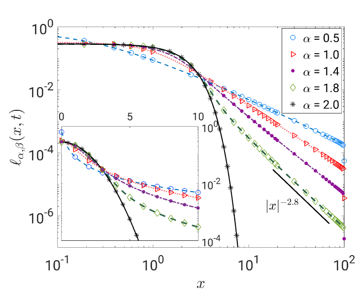
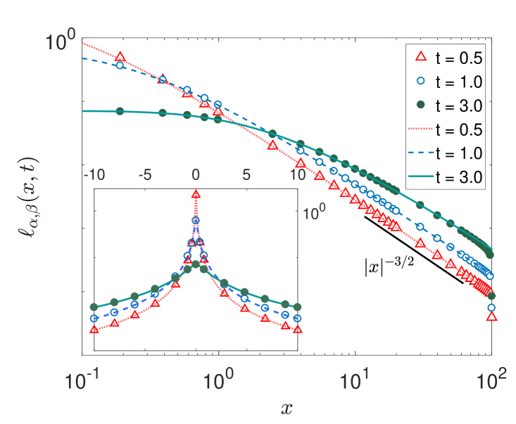
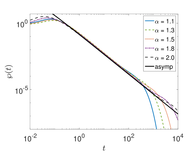
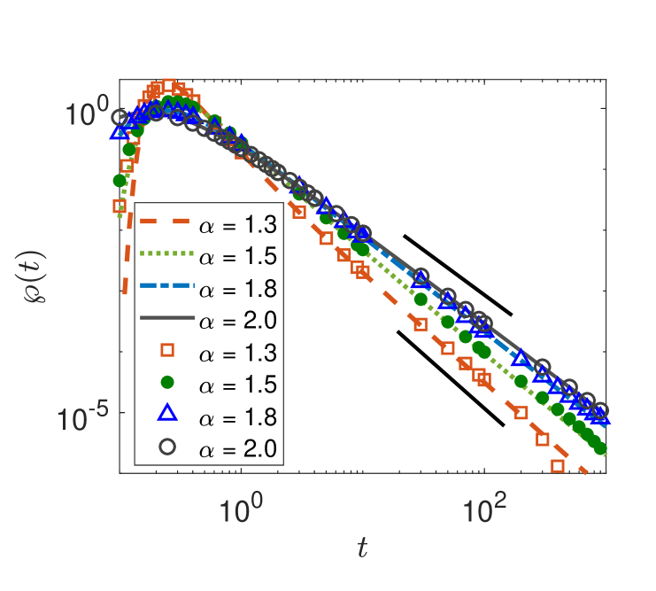
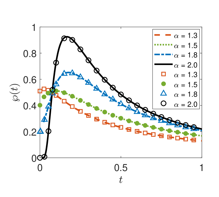
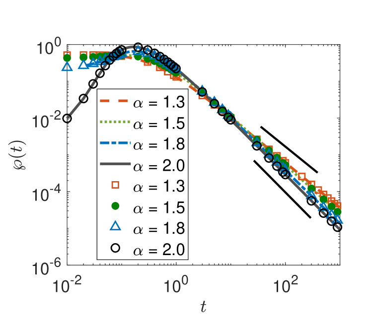
We use absorbing boundary conditions and a finite domain with half length $L=100$ in one dimension, the initial condition is a Dirac $\delta$ -function located at $x(0)=0$ . The probability density function for $\beta=0$ and different sets of the index of stability $\alpha$ at $t=1$ is displayed in figure 1 on the left. The tails display the correct power-law scaling. In the right panel of figure 1 we show the PDF for $\alpha=0.5$ and $\beta=0$ at different times. The insets focus on the central part of the PDFs. In all cases and over the entire plotted range the agreement between the numerical solutions and the theoretical densities is excellent.

3.3.2 Asymmetric $\alpha$ -stable distributions.

Asymmetric stable distributions with non-zero values of the skewness $\beta$ may occur in various situations, for instance, when in a random walk the left and right diffusion coefficients are different. In figure 2 (top) we plot the PDF with $\alpha=1/2$ at $t=1$ for different values of the skewness parameter $\beta$ . On the left side in the main panel the negative side of the tails is shown, on the right side we display the positive side of the tails. Figure 2 (bottom) analogously shows the PDF for $\alpha=1.3$ and different $\beta$ at time $t=1$ . Note that for $\beta=1$ and $0<\alpha<1$ the PDF is completely one-sided on the positive axis and does not possess a left tail.

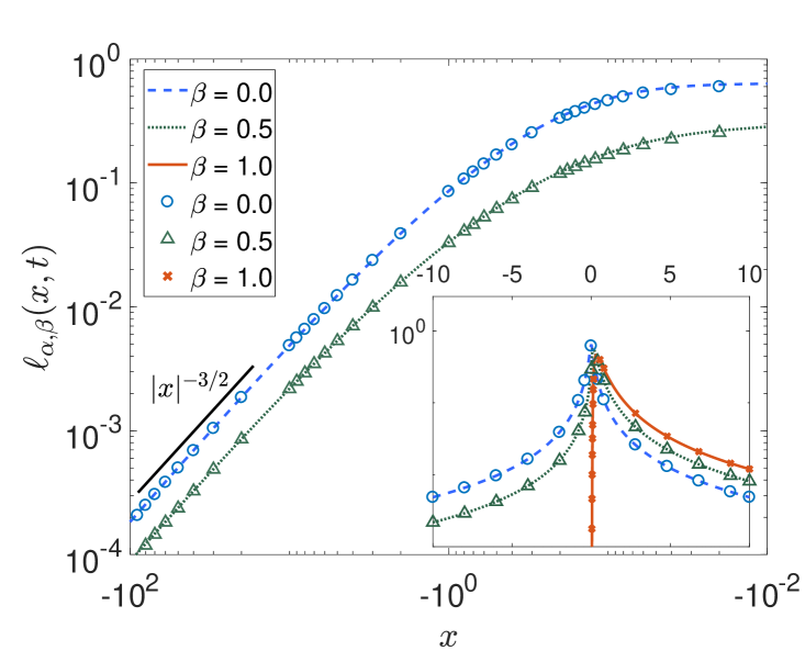
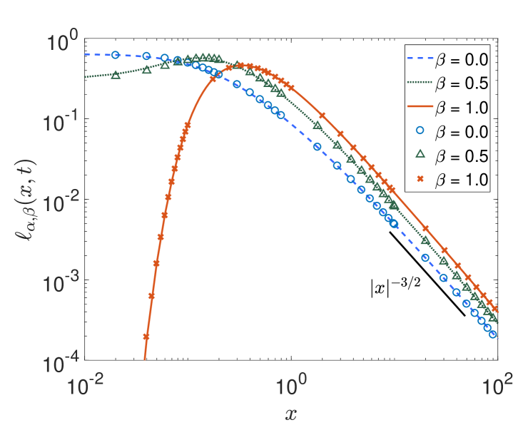
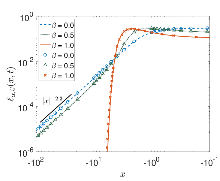
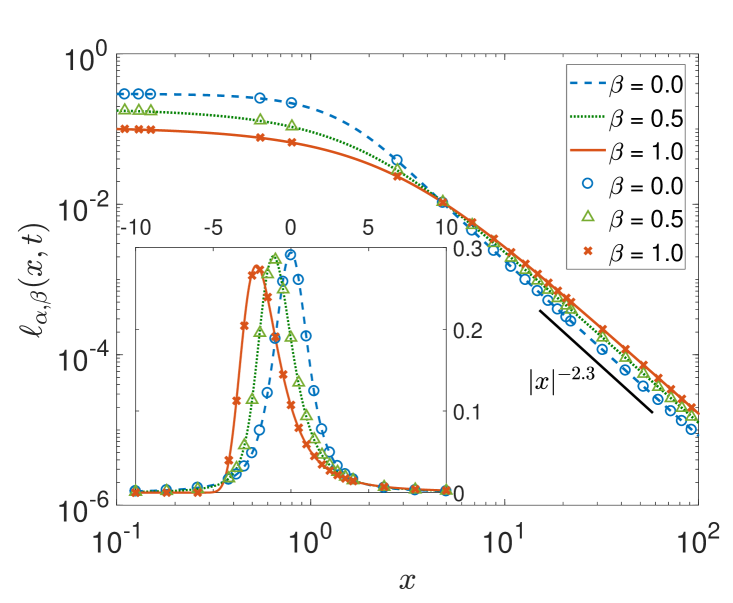
By comparison we see that again the numerical scheme for solving the space-fractional diffusion equation produces solutions that are in very good agreement with the numerical results for the $\alpha$ -stable laws. In the following we study the first-passage properties of random walk processes with $\alpha$ -stable jump length distribution obtained from two numerical methods: the space-fractional diffusion equation and the Langevin approach. We also compare the numerical method for solving the space-fractional diffusion equation with results following from Skorokhod’s theorem.

4 Survival probability and first-passage properties

The survival probability and the first-passage time are observable statistical quantities characterising the stochastic motion in bounded domains with absorbing boundary conditions. In the following we investigate the properties of the survival probability and the first-passage time density in a finite interval for symmetric and asymmetric $\alpha$ -stable laws underlying the space-fractional diffusion equation. To this end we use the setup shown in figure 3, in which absorbing boundaries are located at $-L$ and $L$ , and the initial point of the initial $\delta$ -distribution is located the distance $d$ away from the right boundary.

The probability that at time $t$ the random walker is still present in the interval $[-L,L]$ is defined as the survival probability [155]

S(t)=\int\limits_{-L}^{L}\ell_{\alpha,\beta}(x,t)\mathrm{d}x,

(3fhmnqu)

and the first-passage time PDF is given by the negative time derivative,

\wp(t)=-\frac{\mathrm{d}S(t)}{\mathrm{d}t}.

(3fhmnqv)

Therefore, in Laplace domain with initial condition $S(0)=1$ the relation between the survival probability and the first-passage time reads

\wp(u)=1-uS(u).

(3fhmnqw)

We now first consider the survival probability for symmetric $\alpha$ -stable laws in a semi-infinite and finite interval and demonstrate how the asymptotic properties change with the length of the interval. Furthermore, we compare the results obtained from the numerical difference scheme in section 3.1 with the Langevin equation approach, before embarking for the study of asymmetric $\alpha$ -stable laws.

4.1 First-passage processes for symmetric $\alpha$ -stable laws

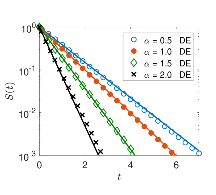
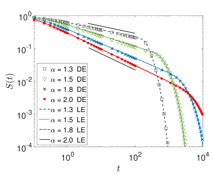
Here we study the properties of $\alpha$ -stable processes in domains restricted by one or two boundaries. In figure 4 we show the survival probability for different $\alpha$ and two different interval lengths $L$ based on the difference scheme solution of the space-fractional diffusion equation and simulations of the Langevin dynamics. The results constructed with both methods are in very good agreement. The data in figure 4 clearly show an exponential decay (in analogy to the escape dynamics of Lévy flights from a confining potential [156, 157]). For the short interval the exponential behaviour sets in almost immediately on the linear time axis in the plot, while for the longer interval a crossover behaviour is visible, as we will see below.

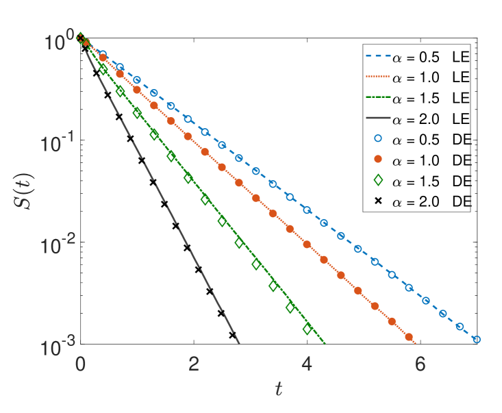
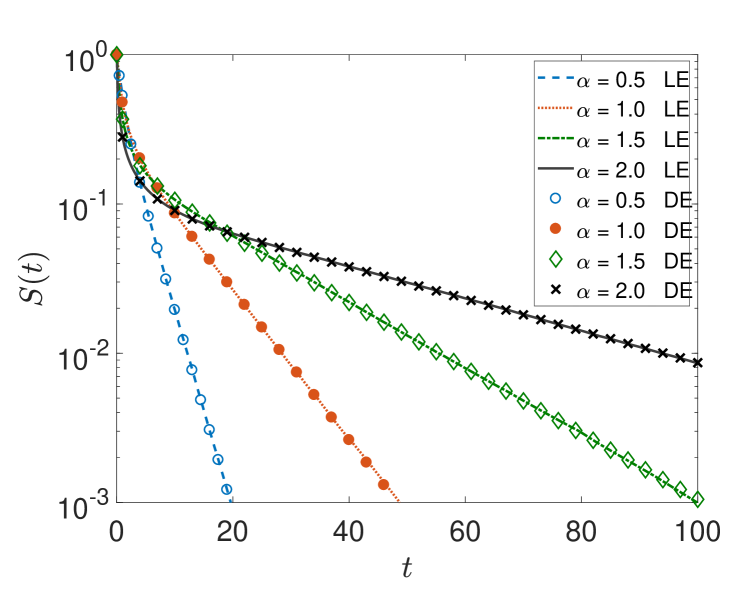
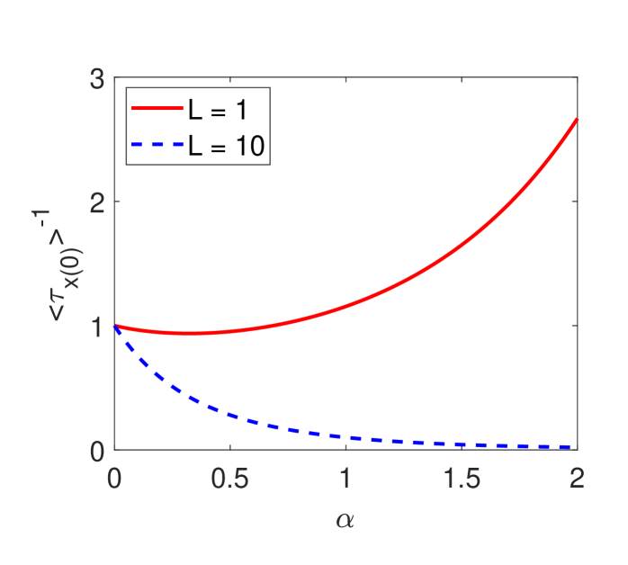
Interestingly, we see in figure 4 that the trend of decay reverses with respect to the stable index $\alpha$ . To understand this behaviour of the survival probability we use the following approximation of the survival probability of symmetric Lévy flights in finite intervals,

S(t|x(0))\approx\exp{\left(-\langle\tau_{x(0)}\rangle^{-1}t\right)},

(3fhmnqx)

where the mean first-passage time

\langle\tau_{x(0)}\rangle=\int_{0}^{\infty}S(t|x(0))\mathrm{d}t

(3fhmnqy)

is given by [158, 159]

\langle\tau_{x(0)}\rangle=\frac{(L^{2}-|x(0)|^{2})^{\alpha/2}}{\Gamma(1+\alpha)K_{\alpha}}.

(3fhmnqz)

Figure 5 compares this approximation with the numerical solution of the space-fractional diffusion equation. As we can see from the left panel, relations (3fhmnqx) and (3fhmnqz) agree very well with the numerical results for $L=1$ : an increase of the interval length $L$ leads to a decrease of $\langle\tau_{x(0)}\rangle^{-1}$ for larger $\alpha$ (right panel of figure 5).

For a semi-infinite domain with absorbing boundary condition it is well known that the first-passage time density for any symmetric jump length distribution in a Markovian setting has the universal Sparre Andersen asymptotic $\wp(t)\simeq t^{-3/2}$ (and thus $S(t)\simeq t^{-1/2}$ [155, 160, 161]. This is exactly our setting here for the symmetric case with $\beta=0$ , and the Sparre Andersen universality was consistently corroborated for symmetric LFs in a number of works, inter alia, [117, 123, 124, 125].

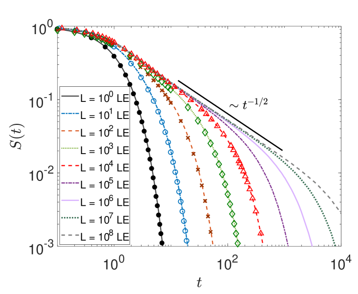
In figure 6 we study what happens at intermediate times in the case of a finite interval, before the terminal exponential shoulder cuts off the survival probability, as shown in figure 4. On the log-log scale of figure 6, we indeed recognise a transient power-law scaling with the universal Sparre Andersen exponent $1/2$ for the survival probability. The onset of the hard exponential cutoff is shifted to longer times with increasing interval size $L$ , in which, on average, it takes the particles longer to explore the full extent of the domain. This, of course, is fully consistent with results for normal diffusion as well as continuous time random walk subdiffusion subordinated to regular random walks [114, 115, 116, 155, 162], compare also the discussion of the area filling dynamics of LFs [163]. Moreover, we see that the results from numerical solution of the fractional diffusion equation and simulations of the Langevin equation almost perfectly agree with each other. The lines without symbols in the top left of figure 6 correspond to cases when the numerical approach based on the fractional diffusion equation did not converge well. We note that one has to increase the value of $L$ with decreasing $\alpha$ in order to meet the Sparre-Andersen scaling for a semi-infinite interval. This is intuitively clear, as smaller $\alpha$ enhances the likelihood of longer jumps and thus effects a higher probability of interaction with the interval boundaries at fixed $L$ .

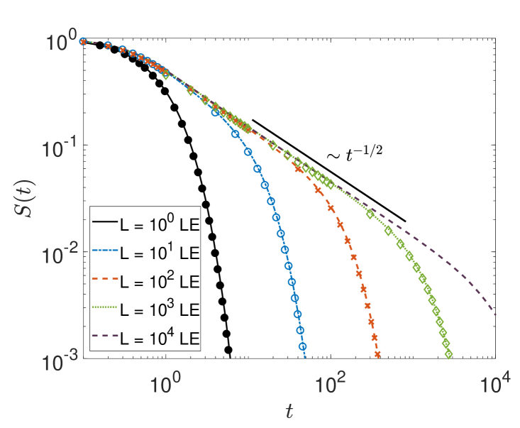
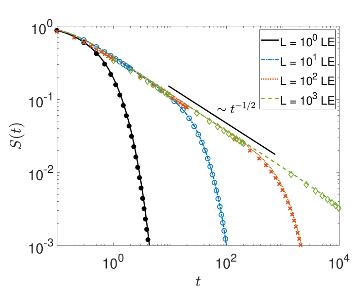
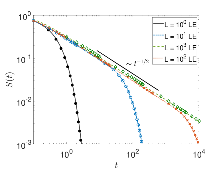
In figure 7 for the interval size $L=100$ we show the survival probability in the left panel along with the the first-passage time density in the right panel, for different $\alpha$ and $\beta=0$ . Consistently, the transient Sparre Andersen scaling is passed on from the power-law exponent $1/2$ for the survival probability to the exponent $3/2$ of the first-passage density.

In the theory of a general class of Lévy processes, that is, homogeneous random processes with independent increments, there exists a theorem, that provides an analytical expression for the PDF of first passage times in a semi-infinite interval, often referred to as the Skorokhod theorem [132, 164]. Based on this theorem the asymptotic expression for symmetric $\alpha$ -stable laws, the first-passage time PDF is (D) [125]

\wp(t)\sim\frac{d^{\alpha/2}}{\alpha\sqrt{\pi K_{\alpha}}\Gamma{(\alpha/2)}}t^{-3/2},

(3fhmnqaa)

which specifies an exact expression for the prefactor of the Sparre Andersen power-law. For Brownian motion ( $\alpha=2$ ), the PDF for the first-passage time has the well known Lévy-Smirnov form [165]

\wp(t)=\frac{d}{\sqrt{4\pi K_{2}t^{3}}}\exp{\left(-\frac{d^{2}}{4K_{2}t}\right)},

(3fhmnqab)

that also emerges from the Skorokhod theorem in the limit $\alpha=2$ . Equation (3fhmnqab) is exact for all times [165, 166], and apart from the Sparre Andersen law $\wp(t)\simeq t^{-3/2}$ it includes the hard short time exponential cutoff reflecting the fact that it takes the particle a typical time $\propto d^{2}/K_{2}$ to reach the absorbing boundary.

4.2 First-passage processes for asymmetric $\alpha$ -stable laws

The case of asymmetric $\alpha$ -stable laws is mathematically more involved and also has been less well studied numerically. We now present results for the survival probability and first-passage time PDF for different skewness parameters $\beta$ , addressing first the special cases of completely one-sided and extremal two-sided laws.

4.2.1 One-sided $\alpha$ -stable laws.

One-sided $\alpha$ -stable laws with $\alpha\in(0,1)$ , $\beta=1$ satisfy the non-negativity of their increments. Physically, such laws are appropriate for jump processes that always move in the same direction, for instance, as a generalisation of shot noise. Applying the Skorokhod theorem to this case one can show that the first-passage time PDF in the permitted interval $\alpha\in(0,1)$ has the exact analytical solution (D) [125]

\wp(t)=\frac{\xi}{d^{\alpha}}M_{\alpha}\left(\frac{\xi t}{d^{\alpha}}\right),

(3fhmnqac)

with

\xi=\frac{K_{\alpha}}{|\cos(\alpha\pi/2)|},

(3fhmnqad)

and where $M_{\alpha}$ is the Wright $M$ -function (also called Mainardi function) [138, 167] with series representation (3fhmnqgg) and asymptotic exponential decay (3fhmnqgi). At sufficiently long times the first-passage time PDF reads

\wp(t)\sim A_{1}(\alpha)t^{(\alpha-1/2)/(1-\alpha)}\exp{(-B_{1}(\alpha)t^{1/(1-\alpha)})},

(3fhmnqae)

where we used the coefficients

A_{1}(\alpha)=\frac{(\alpha\xi/d^{\alpha})^{1/(2-2\alpha)}}{\alpha\sqrt{2\pi(1-\alpha)}},\quad B_{1}(\alpha)=\frac{1-\alpha}{\alpha}(\alpha\xi/d^{\alpha})^{1/(1-\alpha)}.

(3fhmnqaf)

From equation (3fhmnqae) we see that for smaller $\alpha$ the first-passage time density decays faster which is intuitively clear since Lévy flights with smaller $\alpha$ feature longer jumps in the positive direction. The value of $\wp(t)$ at $t=0$ ,

\wp(t=0)=\frac{\xi}{\Gamma{(1-\alpha)}d^{\alpha}},

(3fhmnqag)

demonstrates that, in contrast to the Gaussian case, the probability density does not vanish at $t=0$ , indicating the possibility of immediate escape.

Using equation (3fhmnqv) the survival probability for $0<\alpha<1$ , $\beta=1$ can be expressed exactly in terms of the Wright function $W_{a,b}$ (see equation (3fhmnqge)) or its series expansion,

S(t)=W_{-\alpha,1}(-\xi t/d^{\alpha})=\displaystyle\sum_{n=0}^{\infty}\frac{(-\xi t/d^{\alpha})^{n}}{n!\Gamma(1-\alpha n)}.

(3fhmnqah)

In the limit $\alpha=1/2$ this expression can be reduced to the simple form

S(t)=1-\mathrm{erf}\left(\frac{K_{1/2}t}{\sqrt{2d}}\right),

(3fhmnqai)

and the corresponding first-passage time density is the half-sided Gaussian [124, 168]

\wp(t)=K_{1/2}\sqrt{\frac{2}{\pi d}}\exp\left(-\frac{(K_{1/2}t)^{2}}{2d}\right).

(3fhmnqaj)

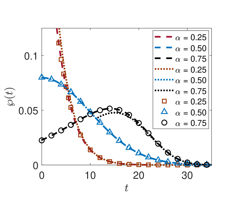
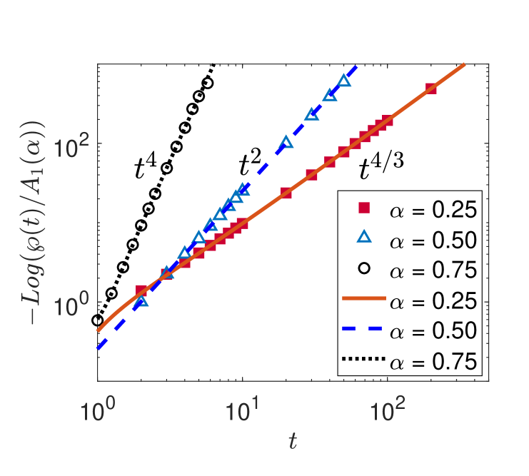
Figure 8 shows numerical and simulations results for $\wp(t)$ , lending excellent support for result (3fhmnqae).

4.2.2 Extremal two-sided $\alpha$ -stable probability laws.

Stable probability laws with stability index $1<\alpha<2$ and skewness $\beta=1$ or $\beta=-1$ are called extremal two-sided skewed $\alpha$ -stable laws. When $\beta=1$ the PDF of an $\alpha$ -stable random variable has a positive power-law tail $x^{-1-\alpha}$ , and a negative tail which is lighter than Gaussian [169], see figure 2. For $\beta=-1$ the properties of the tails are exchanged. In D (see equation (3fhmnqei)) by applying the Skorokhod theorem it is shown that for $\beta=-1$ the PDF of the first-passage time for extremal two-sided stable probability laws has the exact form

\wp(t)=\frac{t^{-1-1/\alpha}d}{\alpha\xi^{1/\alpha}}M_{1/\alpha}\left(\frac{d}{(\xi t)^{1/\alpha}}\right)

(3fhmnqak)

in terms of the Wright $M$ -function $M_{1/\alpha}$ . In the limit $\alpha=2$ we recover the PDF (3fhmnqab) for a Gaussian process. Moreover by using equation (3fhmnqv) the survival probability can be transformed to

S(t)=1-W_{-1/\alpha,1}\left(-\frac{d}{(\xi t)^{1/\alpha}}\right)=\displaystyle\sum_{n=1}^{\infty}\frac{(-1)^{n-1}d^{n}(\xi t)^{-n/\alpha}}{n!\Gamma(1-n/\alpha)}.

(3fhmnqal)

Equation (3fhmnqak) has the following limiting behaviours: at short times $t\to 0$ corresponding to the asymptotic of large argument in the Wright function, by using the asymptotic expression (3fhmnqgi) we find

\wp(t)\sim A_{2}(\alpha)t^{-\frac{2\alpha-1}{2\alpha-2}}\exp{(-B_{2}(\alpha)t^{-\frac{1}{\alpha-1}})},

(3fhmnqam)

where

A_{2}(\alpha)=\frac{(\alpha\xi/d^{\alpha})^{-1/(2\alpha-2)}}{\sqrt{2\pi(\alpha-1)}},\quad B_{2}(\alpha)=(\alpha-1)(\alpha^{\alpha}\xi/d^{\alpha})^{-1/(\alpha-1)}.

(3fhmnqan)

At long times, $t\to\infty$ ,

\wp(t)\sim\frac{\xi^{-1/\alpha}d}{\alpha\Gamma{(1-1/\alpha)}}t^{-1-1/\alpha},

(3fhmnqao)

consistent with the result in [124].

For the extremal two-sided $\alpha$ -stable probability laws with index $1<\alpha<2$ and skewness $\beta=1$ , by using the Skorokhod theorem the PDF of first-passage times has the following series representation (see D, equation (3fhmnqfa))

\wp(t)=\frac{t^{-2+1/\alpha}d^{\alpha-1}}{\alpha\xi^{1-1/\alpha}}\displaystyle\sum_{n=1}^{\infty}\frac{({\xi t/d^{\alpha}})^{-n+1}}{\Gamma{(\alpha n-1)}\Gamma{(1+1/\alpha-n)}}.

(3fhmnqap)

For $\alpha=2$ we again consistently recover result (3fhmnqab). The asymptotic behaviour of equation (3fhmnqap) at long times is

\wp(t)\sim\frac{\xi^{-1+1/\alpha}d^{\alpha-1}}{\alpha\Gamma{(\alpha-1)}\Gamma{(1/\alpha)}}t^{-2+1/\alpha},

(3fhmnqaq)

and in the limit $t\to 0$ , we find the finite value

\wp(0)=-\frac{\xi d^{-\alpha}}{\Gamma{(1-\alpha)}}.

(3fhmnqar)

By using the relation between the survival probability and the first-passage time PDF in Laplace space (equation (3fhmnqw)) and applying the inverse Laplace transform we obtain a series representation for the survival probability for extremal two-sided $\alpha$ -stable probability laws ( $1<\alpha<2$ , $\beta=1$ ) in the form

S(t)=\displaystyle\sum_{n=1}^{\infty}\frac{(\xi t)^{1/\alpha-n}d^{n\alpha-1}}{\Gamma{(\alpha n)}\Gamma(1-n+1/\alpha)}.

(3fhmnqas)

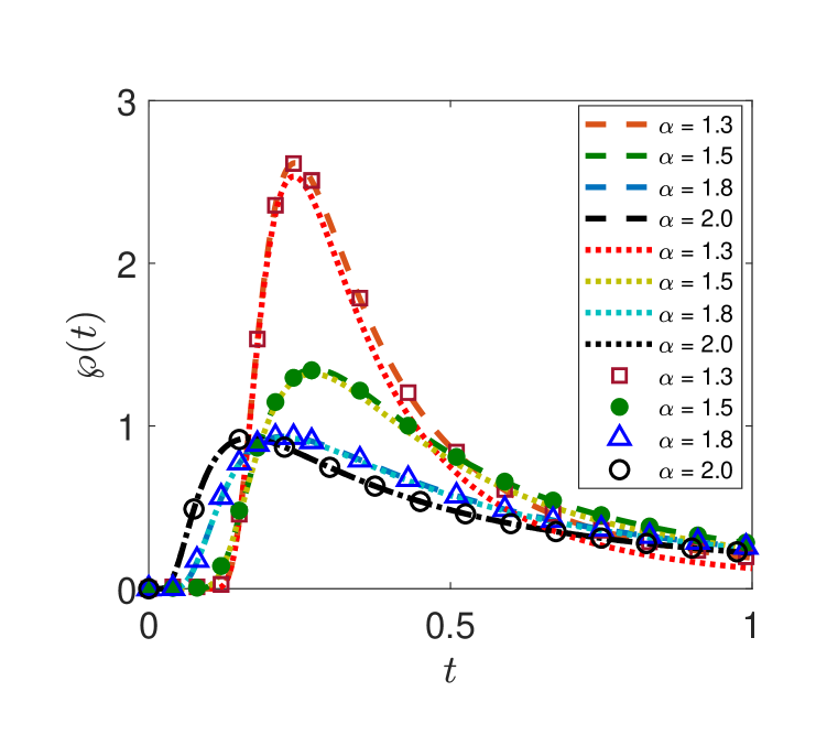
The first-passage time PDFs for extremal two-sided $\alpha$ -stable probability laws are displayed in figure 9.

4.2.3 $\alpha$ -stable probability laws in general asymmetric form.

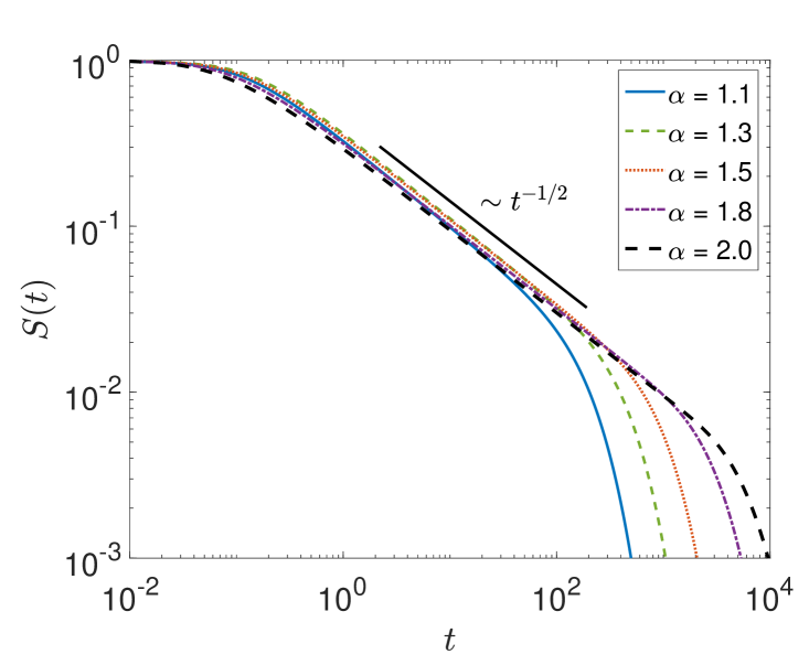
We finally study the first-passage behaviour for asymmetric Lévy stable laws of arbitrary skewness $\beta$ , again based on the comparison between the numerical solution of the space-fractional diffusion equation and simulations of the Langevin approach for different stable index $\alpha$ . The results are shown in log-log scale in figures 10 and 11 in the range $1<\alpha<2$ . Figure 10 depicts the cases $\beta=1$ and $\beta=-1$ , while figure 11 shows the cases $\beta=0.5$ and $\beta=-0.5$ . As can be seen from both figures, a positive value of the skewness leads to a slower decay (shallower slope) than for the Gaussian case, and opposite for negative values of $\beta$ . Indeed, this behaviour is not immediately intuitive, as a positive skewness means that the stable law has a longer tail on the positive axis. However, what matters for the short and intermediate first-passage time scales are values of the stable law around the most likely value, and for positive skewness this is located on the negative axis (compare bottom panels in figure 2). Thus, Lévy flights with a positive skewness experience an effective drift to the left, in our setting away from the absorbing boundary.

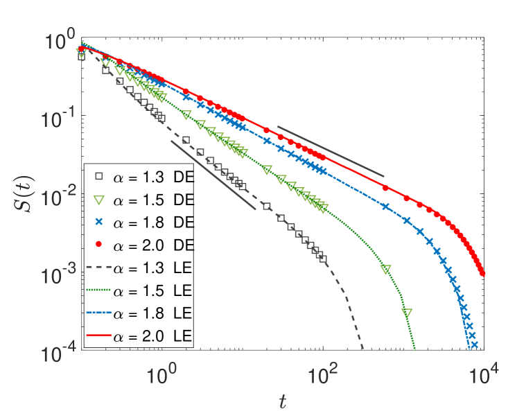
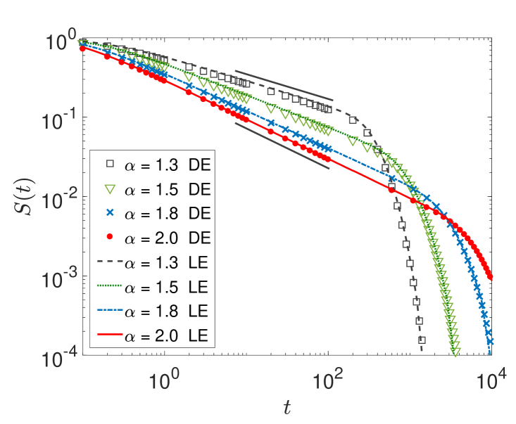
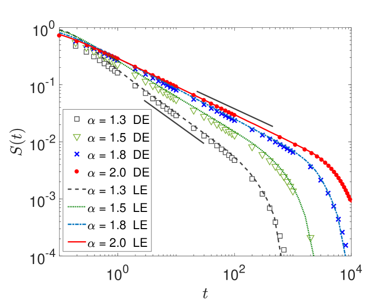
From the Skorokhod theorem for $\alpha\in(0,1)$ and $\beta\in(-1,1)$ , $\alpha=1$ and $\beta=0$ , as well as $\alpha\in(1,2]$ and $\beta\in[-1,1]$ we obtained the power-law decay (see D.6)

\wp(t)\sim\frac{\rho(K_{\alpha}(1+\beta^{2}\tan^{2}{(\alpha\pi/2)})^{1/2})^{-\rho}d^{\alpha\rho}}{\Gamma(1-\rho)\Gamma(1+\alpha\rho)}t^{-\rho-1},

(3fhmnqat)

where the positive parameter $\rho$ is defined as

\rho=\frac{1}{2}+\frac{1}{\pi\alpha}\arctan(\beta\tan(\pi\alpha/2)).

(3fhmnqau)

Following [170] (page 218) we write this in a form with a general $\beta$ . This is the direct generalisation of the classical Sparre Andersen universality for asymmetric stable jump length distributions. It is easy to check that this result reduces to the known cases for vanishing skewness. We note that the inapplicability of the Sparre Andersen law for asymmetric jump length distributions was already pointed out by Spitzer ([171], page 227). The analytical predictions from relations (3fhmnqat) and (3fhmnqau) are in excellent agreement with the data shown in figures 10 and 11.

5 Discussion and unsolved problems

LFs are Markovian stochastic processes that are commonly used across disciplines as models for jump processes that exhibit the distinct propensity for very long jumps. The scale-free nature of the underlying, Lévy stable PDF of jump lengths with its heavy power-law tail has been shown to effect a more efficient random search strategy than the more conventional Brownian search processes. We here combined numerical inversion methods of the solution of the space-fractional diffusion equation and simulation of the Langevin equation fuelled by $\alpha$ -stable white noise to quantify the first-passage dynamics of LFs with a general asymmetric jump length PDF. In particular, we demonstrated that in all cases both approaches are in excellent agreement. As both approaches have advantages and disadvantages, it is very useful to have available two equally potent methods. In addition, we verified the crossover to an exponential behaviour of the first-passage time PDF in a finite domain and the existence of a well-established power-law decay at intermediate times, before the random walker explores the full range of the finite domain and thus behaves as if it were in a semi-infinite range. For symmetric $\alpha$ -stable laws this decay was shown to be fully consistent with the expected Sparre Andersen universal law. For asymmetric cases, when the conditions of the Sparre Andersen theorem are no longer fulfilled, we derived the analytical behaviour from the Skorokhod theorem for specific values of the skewness. In the general case the direct extension of this analytical law was shown to be fully consistent with the numerical and simulations results. The results obtained here will be of use in applications, as these typically are involved with search processes and thus measure first-passage times. Concurrently, these results also further complete the mathematical theory of Lévy stable processes.

$\alpha$	$\beta$	Exact PDF	Long-time asymptotic	Prefactor
		Equation		Equation
2	Irrelevant	$\frac{d}{\sqrt{4\pi K_{2}t^{3}}}\exp\left(-\frac{d^{2}}{4K_{2}t}\right)$ (3fhmnqab) [165]
(0,2)	0	Unknown	$\simeq t^{-3/2}$ [127, 128]	(3fhmnqaa) [125]
(0,1)	1	(3fhmnqac) [125]	$\sim A_{1}(\alpha)t^{(\alpha-1/2)/(1-\alpha)}\exp[-B_{1}(\alpha)t^{1/(1-\alpha)}]$	(3fhmnqaf) [125]
$1/2$	1	$K_{\alpha}\sqrt{2/\pi d}\exp[-(K_{\alpha}t)^{2}/2d]$ (3fhmnqaj) [124, 125, 168]
(1,2)	-1	(3fhmnqak)	$\simeq t^{-1-1/\alpha}$ [124]	(3fhmnqao) [172]²²2Note that the result (3fhmnqao) differs from that of [172] by a factor which appears due to the use of two different forms of the characteristic function for the $\alpha$ -stable process.
(1,2)	1	(3fhmnqap)	$\simeq t^{-2+1/\alpha}$	(3fhmnqaq)
(0,1)	(-1,1)	Unknown	$\simeq t^{-3/2-(\pi\alpha)^{-1}\tan^{-1}[\beta\tan(\pi\alpha/2)]}$ [170]	(3fhmnqat) [173, 174]
(1,2)	(-1,1)	Unknown		(3fhmnqat) [173, 174]

Table 1: First-passage time PDF for different stable indices

\alpha

and skewness parameters

\beta

. The fifth column refers to the equation number for the full prefactor of the asymptotic law in column four. ²²footnotetext: Note that the result (3fhmnqao) differs from that of [172] by a factor which appears due to the use of two different forms of the characteristic function for the

\alpha

-stable process.

The first-passage time properties of general $\alpha$ -stable probability laws are summarised in table 1. For the known cases we include the references to the relevant equations of the exact PDF as well as the asymptotic prefactor. Some special cases are included, as well. Those cases with previously known results refer to the relevant references.

It is possible to extend the studied setup to higher dimensions [175, 176, 177, 178]. In this case, the scalar noise term $\zeta(t)$ in the Langevin equation (3fhmnqr) for $x(t)$ is replaced by multivariate Lévy noise in the higher-dimensional Langevin equation for $\mathbf{x}(t)$ . Here, multivariate $\alpha$ -stable variables are characterised by a spectral measure defined on the unit circle [18]. For the numerical scheme of the multi-dimensional space-fractional diffusion equation we refer to [179, 180, 181, 182, 183, 184, 185, 186]. We note that to the best knowledge of the authors no multi-dimensional generalisation of Skorokhod’s theorem exists. Thus, the extension of the analytical and numerical approaches presented here to higher dimensions represents a challenging problem requiring further studies.

Generally the formulation of non-local and/or correlated stochastic processes is not always an easy task and, in some cases, still not fully understood. Apart from LFs, we may allude to the debate on the formulation and solution of boundary value problems for fractional Brownian motion, a process fuelled with Gaussian yet long-range correlated noise [187, 188, 189]. For LFs, in addition to the results obtained here it will be interesting to generalise the results obtained for symmetric $\alpha$ -stable laws in the presence of an external drift in [113]. Similarly, it will be of interest to investigate the PDF of first arrival times, related to the probability of hitting a small target in an otherwise unbounded environment, for the general case of asymmetric Lévy stable laws.

AP acknowledges funding from the Ministry of Science, Research and Technology of Iran and University of Potsdam. This research was supported in part by PLGrid Infrastructure. The computer simulations were performed at Potsdam University and the Academic Computer Center Cyfronet, Akademia Górniczo-Hutnicza (Kraków, Poland) under CPU grant DynStoch. AC and RM acknowledge support from DFG project ME 1535/7-1. RM also thanks the Foundation for Polish Science for support within an Alexander von Humboldt Polish Honorary Research Scholarship.

Appendix A Parametrisation of characteristic function for $\alpha$ -stable processes

There are several forms for the parametrisation of $\alpha$ -stable laws appearing in literature, basically because of historical reasons. Each form might be useful in a particular situation. For example, one of them is preferable for analytical calculations, whereas the other ones can be more convenient for numerical purposes or for fitting of data. Following the exposition of the various forms of stable laws in [154, 190], we here present four parameterisation forms for the characteristic functions.

In the main text we use the A-form of the characteristic function,

\hat{\ell}_{\alpha,\beta_{A}}^{A}(k,t)=\exp\Big{(}-tK_{\alpha}^{A}|k|^{\alpha}[1-\mathrm{i}\beta_{A}\mathrm{sgn}(k)\omega_{A}(k,\alpha)]+\mathrm{i}\mu_{A}kt\Big{)},

(3fhmnqav)

where

\omega_{A}(k,\alpha)=\left\{\begin{array}[]{ll}\tan(\frac{\pi\alpha}{2}),&\alpha\neq 1,\\ -\frac{2}{\pi}\ln|k|,&\alpha=1\end{array}\right..

(3fhmnqaw)

In this paper we exclude the case $\alpha=1$ and $\beta\neq 0$ . The B-form is helpful from an analytical point of view, it is given by

\hat{\ell}_{\alpha,\beta_{B}}^{B}(k,t)=\exp\Big{(}-tK_{\alpha}^{B}|k|^{\alpha}\omega_{B}(k,\alpha,\beta_{B})+\mathrm{i}\mu_{B}kt\Big{)},

(3fhmnqax)

where (for $\alpha\neq 1$ )

\omega_{B}(k,\alpha,\beta_{B})=\exp\Big{(}-\mathrm{i}\frac{\pi}{2}\beta_{B}K(\alpha)\mathrm{sgn}(k)\Big{)}

(3fhmnqay)

and $K(\alpha)=\alpha-1+\mathrm{sgn}(1-\alpha)$ . The parameters have the same domains of variation as in the A-form,

\beta_{A}=\cot\left(\frac{\alpha\pi}{2}\right)\tan\left(\beta_{B}K(\alpha)\frac{\pi}{2}\right),\quad\mu_{A}=\mu_{B},K_{\alpha}^{A}=\cos\left(\beta_{B}K(\alpha)\frac{\pi}{2}\right)K_{\alpha}^{B}.

(3fhmnqaz)

The M-form is used in numerical simulations and reads

\hat{\ell}_{\alpha,\beta_{M}}^{M}(k,t)=\exp\Big{(}-tK_{\alpha}^{M}|k|^{\alpha}[1+\mathrm{i}\beta_{M}\mathrm{sgn}(k)\omega_{M}(k,\alpha,t)]+\mathrm{i}\mu_{M}(t)kt\Big{)},

(3fhmnqba)

where ( $\alpha\neq 1$ )

\omega_{M}(k,\alpha,t)=\tan\left(\frac{\pi\alpha}{2}\right)\left[(K_{\alpha}^{M}t)^{1/\alpha-1}|k|^{1-\alpha}-1\right].

(3fhmnqbb)

The domain of variation of the parameters in the A- and M-forms is the same and connected by the following relations

\beta_{M}=\beta_{A},\quad\mu_{M}(t)=\mu_{A}+\frac{(K_{\alpha}^{A}t)^{1/\alpha}}{t}\beta_{A}\tan\left(\frac{\pi\alpha}{2}\right),\quad K_{\alpha}^{M}=K_{\alpha}^{A}.

(3fhmnqbc)

Finally, the Z-form is represented by

\hat{\ell}_{\alpha,\rho}^{Z}(k,t)=\exp\Big{(}-tK_{\alpha}^{Z}(\mathrm{i}k)^{\alpha}\exp\left[-\mathrm{i}\pi\alpha\rho\mathrm{sgn}(k)\right]\Big{)},

(3fhmnqbd)

where the parameters $\alpha$ and $\rho$ vary within the bounds

0<\alpha\leq 2,1-\min(1,1/\alpha)\leq\rho\leq\min(1,1/\alpha),\quad t>0,

(3fhmnqbe)

and the relation between the parameters in the A- and Z-forms is as follows,

\rho=\frac{1}{2}+\frac{1}{\alpha\pi}\arctan\left(\beta_{A}\tan\left(\frac{\alpha\pi}{2}\right)\right),\quad K_{\alpha}^{Z}=K_{\alpha}^{A}\left(1+\left[\beta_{A}\tan\left(\frac{\alpha\pi}{2}\right)\right]^{2}\right)^{1/2}.

(3fhmnqbf)

In the A-, B-, and M-forms $\beta_{A}=1$ corresponds to $\beta_{M}=1$ and $\beta_{B}=1$ , while in the case of the Z-form the value $\beta_{A}=1$ corresponds to the value $\rho=1$ if $\alpha<1$ and to the value $\rho=1-1/\alpha$ if $\alpha>1$ .

Appendix B Some details of the numerical scheme

With the use of equations (3e) and (3fhl) we can write equation (3d) on a discrete space-time grid as

\frac{f_{i}^{j+1}-f_{i}^{j}}{\Delta t}=K_{\alpha}\left[L_{\alpha,\beta}\,{}_{a}D_{x}^{\alpha}D{f(x_{i},t_{j})}+R_{\alpha,\beta}\,{}_{x}D_{b}^{\alpha}D{f(x_{i},t_{j})}\right].

(3fhmnqbg)

Here we consider discretisation schemes for the three cases $0<\alpha<1$ , $1<\alpha\leq 2$ , and $\alpha=1$ separately.

B.1 $0<\alpha<1$

By substitution of equations (3fhl) to (3fhmb) into equation (3fhmnqbg) and using the relation

\int\limits_{a}^{b}\frac{1}{[\pm(x-y)]^{\gamma}}\mathrm{d}y=\frac{1}{\pm(\gamma-1)}\left[(\pm(x-b))^{1-\gamma}-(\pm(x-a))^{1-\gamma}\right]

(3fhmnqbh)

where the sign $+$ is taken for $x>b>a$ and $-$ for $x<a<b$ , we obtain

	$\displaystyle\frac{f_{i}^{j+1}-f_{i}^{j}}{\Delta t}$	$\displaystyle=$	$\displaystyle K_{\alpha}\left[\frac{L_{\alpha,\beta}}{\Gamma(2-\alpha)}\displaystyle\sum_{k=1}^{i}\frac{f_{k}^{j}-f_{k-1}^{j}}{\Delta x}\left((x_{i}-x_{k-1})^{1-\alpha}-(x_{i}-x_{k})^{1-\alpha}\right)\right.$		(3fhmnqbj)
			$\displaystyle\left.+\frac{R_{\alpha,\beta}}{\Gamma(2-\alpha)}\displaystyle\sum_{k=i}^{I-1}\frac{f_{k}^{j}-f_{k+1}^{j}}{\Delta x}\left((x_{k+1}-x_{i})^{1-\alpha}-(x_{k}-x_{i})^{1-\alpha}\right)\right].$		(3fhmnqbj)

Defining

\lambda_{n}=n^{1-\alpha}-(n-1)^{1-\alpha},\quad\Omega_{L}=\frac{L_{\alpha,\beta}K_{\alpha}\Delta t}{\Gamma(2-\alpha)(\Delta x)^{\alpha}},\quad\Omega_{R}=\frac{R_{\alpha,\beta}K_{\alpha}\Delta t}{\Gamma(2-\alpha)(\Delta x)^{\alpha}},

(3fhmnqbk)

we rewrite equation (3fhmnqbj) as

f_{i}^{j+1}-f_{i}^{j}=\Omega_{L}\displaystyle\sum_{k=1}^{i}\left(f_{k}^{j}-f_{k-1}^{j}\right)\lambda_{i-k+1}+\Omega_{R}\displaystyle\sum_{k=i}^{I-1}\left(f_{k}^{j}-f_{k+1}^{j}\right)\lambda_{k-i+1}.

(3fhmnqbl)

Changing $f_{i}\to\theta f_{i}^{j+1}+(1-\theta)f_{i}^{j}$ , $0\leq\theta\leq 1$ , on the right hand side,

	$\displaystyle-\theta\Omega_{L}\displaystyle\sum_{k=1}^{i}\left(f_{k}^{j+1}-f_{k-1}^{j+1}\right)\lambda_{i-k+1}+f_{i}^{j+1}-\theta\Omega_{R}\displaystyle\sum_{k=i}^{I-1}\left(f_{k}^{j+1}-f_{k+1}^{j+1}\right)\lambda_{k-i+1}$
	$\displaystyle=(1-\theta)\Omega_{L}\displaystyle\sum_{k=1}^{i}\left(f_{k}^{j}-f_{k-1}^{j}\right)\lambda_{i-k+1}+f_{i}^{j}+(1-\theta)\Omega_{R}\displaystyle\sum_{k=i}^{I-1}\left(f_{k}^{j}-f_{k+1}^{j}\right)\lambda_{k-i+1}.$		(3fhmnqbm)

Then the matrices $\mathbf{A}$ and $\mathbf{B}$ in equation (3fhmnp) are

\mathbf{A}=\left(\begin{array}[]{cccc}A_{c}&A_{1,R}&\cdots&A_{I,R}\\ A_{1,L}&\ddots&\ddots&\vdots\\ \vdots&\ddots&\ddots&A_{1,R}\\ A_{I,L}&\cdots&A_{1,L}&A_{c}\end{array}\right),\qquad\mathbf{B}=\left(\begin{array}[]{cccc}B_{c}&B_{1,R}&\cdots&B_{I,R}\\ B_{1,L}&\ddots&\ddots&\vdots\\ \vdots&\ddots&\ddots&B_{1,R}\\ B_{I,L}&\cdots&B_{1,L}&B_{c}\end{array}\right),

(3fhmnqbn)

where

\begin{array}[]{ll}A_{c}=1-\theta(\Omega_{L}+\Omega_{R})\lambda_{1}\\ A_{i,L}=\theta\Omega_{L}(\lambda_{i}-\lambda_{i+1}),\quad i=1,2,\ldots,I\\ A_{i,R}=\theta\Omega_{R}(\lambda_{i}-\lambda_{i+1}),\quad i=1,2,\ldots,I\end{array}

(3fhmnqbo)

and

\begin{array}[]{ll}B_{c}=1+(1-\theta)(\Omega_{L}+\Omega_{R})\lambda_{1}\\ B_{i,L}=-(1-\theta)\Omega_{L}(\lambda_{i}-\lambda_{i+1}),\quad i=1,2,\ldots,I\\ B_{i,R}=-(1-\theta)\Omega_{R}(\lambda_{i}-\lambda_{i+1}),\quad i=1,2,\ldots,I.\end{array}

(3fhmnqbp)

B.2 $1<\alpha<2$

Substituting equations (3fhl), (3fhmna), and (3fhmnb) into equation (3fhmnqbg) we get

	$\displaystyle\frac{f_{i}^{j+1}-f_{i}^{j}}{\Delta t}$	$\displaystyle=$	$\displaystyle K_{\alpha}\left[\frac{L_{\alpha,\beta}}{\Gamma(3-\alpha)}\displaystyle\sum_{k=1}^{i}\frac{f_{k+1}^{j}-2f_{k}^{j}+f_{k-1}^{j}}{(\Delta x)^{2}}\left((x_{i}-x_{k-1})^{2-\alpha}-(x_{i}-x_{k})^{2-\alpha}\right)\right.$		(3fhmnqbq)
			$\displaystyle\hskip-34.14322pt+\left.\frac{R_{\alpha,\beta}}{\Gamma(3-\alpha)}\displaystyle\sum_{k=i}^{I-1}\frac{f_{k+1}^{j}-2f_{k}^{j}+f_{k-1}^{j}}{(\Delta x)^{2}}\left((x_{k+1}-x_{i})^{2-\alpha}-(x_{k}-x_{i})^{2-\alpha}\right)\right]$		(3fhmnqbq)

with the definition

\lambda_{n}=n^{2-\alpha}-(n-1)^{2-\alpha},\quad\Omega_{L}=\frac{L_{\alpha,\beta}K_{\alpha}\Delta t}{\Gamma(3-\alpha)(\Delta x)^{\alpha}},\quad\Omega_{R}=\frac{R_{\alpha,\beta}K_{\alpha}\Delta t}{\Gamma(3-\alpha)(\Delta x)^{\alpha}},

(3fhmnqbr)

and changing the notation as above, we obtain

	$\displaystyle-\theta\Omega_{L}\displaystyle\sum_{k=1}^{i}\left(f_{k+1}^{j+1}-2f_{k}^{j+1}+f_{k-1}^{j+1}\right)\lambda_{i-k+1}+f_{i}^{j+1}$	(3fhmnqbs)
	$\displaystyle-\theta\Omega_{R}\displaystyle\sum_{k=i}^{I-1}\left(f_{k+1}^{j+1}-2f_{k}^{j+1}+f_{k-1}^{j+1}\right)\lambda_{k-i+1}$
$\displaystyle=$	$\displaystyle(1-\theta)\Omega_{L}\displaystyle\sum_{k=1}^{i}\left(f_{k+1}^{j}-2f_{k}^{j}+f_{k-1}^{j}\right)\lambda_{i-k+1}+f_{i}^{j}$
	$\displaystyle+(1-\theta)\Omega_{R}\displaystyle\sum_{k=i}^{I-1}\left(f_{k+1}^{j}-2f_{k}^{j}+f_{k-1}^{j}\right)\lambda_{k-i+1}.$

Then the elements of the matrix A and B in equation (3fhmnp) are

\begin{array}[]{ll}A_{c}=1-\theta(\Omega_{L}+\Omega_{R})(\lambda_{2}-2\lambda_{1})\\ A_{1,L}=-\theta\Omega_{L}(\lambda_{3}-2\lambda_{2}+\lambda_{1})-\theta\Omega_{R}\lambda_{1}\\ A_{1,R}=-\theta\Omega_{R}(\lambda_{3}-2\lambda_{2}+\lambda_{1})-\theta\Omega_{L}\lambda_{1}\\ A_{i,L}=-\theta\Omega_{L}(\lambda_{i+2}-2\lambda_{i+1}+\lambda_{i}),\quad i=2,3,\ldots,I\\ A_{i,R}=-\theta\Omega_{R}(\lambda_{i+2}-2\lambda_{i+1}+\lambda_{i}),\quad i=2,3,\ldots,I\end{array}

(3fhmnqbt)

and

\begin{array}[]{ll}B_{c}=1+(1-\theta)(\Omega_{L}+\Omega_{R})(\lambda_{2}-2\lambda_{1})\\ B_{1,L}=(1-\theta)\Omega_{L}(\lambda_{3}-2\lambda_{2}+\lambda_{1})+(1-\theta)\Omega_{R}\lambda_{1}\\ B_{1,R}=(1-\theta)\Omega_{R}(\lambda_{3}-2\lambda_{2}+\lambda_{1})+(1-\theta)\Omega_{L}\lambda_{1}\\ B_{i,L}=(1-\theta)\Omega_{L}(\lambda_{i+2}-2\lambda_{i+1}+\lambda_{i}),\quad i=2,3,\ldots,I\\ B_{i,R}=(1-\theta)\Omega_{R}(\lambda_{i+2}-2\lambda_{i+1}+\lambda_{i}),\quad i=2,3,\ldots,I\end{array}.

(3fhmnqbu)

B.3 $\alpha=1$ , $\beta=0$

By substituting equations (3fhmno) and (3fhl) into equation (3fhi) we obtain

\displaystyle\frac{f_{i}^{j+1}-f_{i}^{j}}{\Delta t}=-\frac{2K_{\alpha}}{\pi}\left[\displaystyle\sum_{k=1}^{i}\frac{f^{j}_{k}-f^{j}_{k-1}}{\Delta x}\frac{1}{2(i-k)+1}+\displaystyle\sum_{k=i}^{I-1}\frac{f^{j}_{k}-f^{j}_{k+1}}{\Delta x}\frac{1}{2(k-i)+1}\right].

(3fhmnqbv)

Defining

\lambda_{n}=\frac{1}{2n+1},\quad\Omega_{L}=\frac{2L_{\alpha,\beta}K_{\alpha}\Delta t}{\Delta x},\quad\Omega_{R}=\frac{2R_{\alpha,\beta}K_{\alpha}\Delta t}{\Delta x},

(3fhmnqbw)

changing notation as above, we obtain

	$\displaystyle\theta\Omega_{L}\displaystyle\sum_{k=1}^{i}\left(f_{k}^{j+1}-f_{k-1}^{j+1}\right)\lambda_{i-k}+f_{i}^{j+1}+\theta\Omega_{R}\displaystyle\sum_{k=i}^{I-1}\left(f_{k}^{j+1}-f_{k+1}^{j+1}\right)\lambda_{k-i}$
	$\displaystyle=-(1-\theta)\Omega_{L}\displaystyle\sum_{k=1}^{i}\left(f_{k}^{j}-f_{k-1}^{j}\right)\lambda_{i-k}+f_{i}^{j}-(1-\theta)\Omega_{R}\displaystyle\sum_{k=i}^{I-1}\left(f_{k}^{j}-f_{k+1}^{j}\right)\lambda_{k-i}.$		(3fhmnqbx)

Then the elements of the matrices A and B in equation (3fhmnp) are

\begin{array}[]{ll}A_{c}=1+\theta(\Omega_{L}+\Omega_{R})\lambda_{0}\\ A_{i,L}=\theta\Omega_{L}(\lambda_{i}-\lambda_{i-1}),\quad i=1,2,\ldots,I\\ A_{i,R}=\theta\Omega_{R}(\lambda_{i}-\lambda_{i-1}),\quad i=1,2,\ldots,I\end{array}

(3fhmnqby)

and

\begin{array}[]{ll}B_{c}=1-(1-\theta)(\Omega_{L}+\Omega_{R})\lambda_{0}\\ B_{i,L}=-(1-\theta)\Omega_{L}(\lambda_{i}-\lambda_{i-1}),\quad i=1,2,\ldots,I\\ B_{i,R}=-(1-\theta)\Omega_{R}(\lambda_{i}-\lambda_{i-1}),\quad i=1,2,\ldots,I.\end{array}

(3fhmnqbz)

Appendix C Error estimation of the difference scheme

We here provide some details on the error estimate of our difference scheme. For the case $0<\alpha<1$ (equation (13))

\int\limits_{-L}^{x_{i}}\frac{f^{(1)}(\zeta,t_{j})}{(x_{i}-\zeta)^{\alpha}}\mathrm{d}\zeta\approx\displaystyle\sum_{k=1}^{i}\frac{f^{j}_{k}-f^{j}_{k-1}}{\Delta x}\int\limits_{x_{k-1}}^{x_{k}}\frac{1}{(x_{i}-\zeta)^{\alpha}}\mathrm{d}\zeta+\mathcal{O}(\Delta x^{2-\alpha}),

(3fhmnqca)

for the left side derivative, and

\int\limits_{x_{i}}^{L}\frac{f^{(1)}(\zeta,t_{j})}{(\zeta-x_{i})^{\alpha}}\mathrm{d}\zeta\approx\displaystyle\sum_{k=i}^{I-1}\frac{f^{j}_{k+1}-f^{j}_{k}}{\Delta x}\int\limits_{x_{k}}^{x_{k+1}}\frac{1}{(\zeta-x_{i})^{\alpha}}\mathrm{d}\zeta+\mathcal{O}(\Delta x^{2-\alpha}),

(3fhmnqcb)

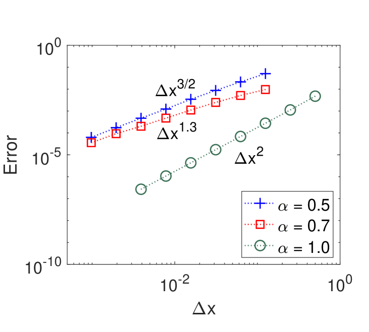
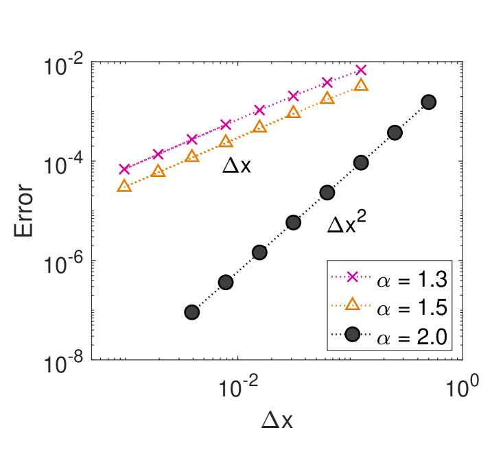
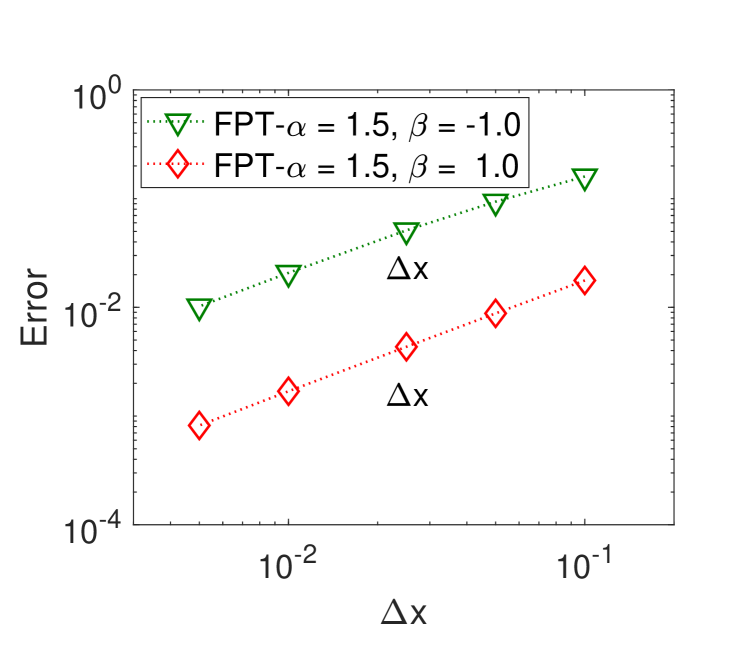
for the right side derivative. This efficient way to approximate the Caputo derivative of order $\alpha$ ( $0<\alpha<1$ ) is called L1 scheme [191, 192, 193] and its error estimate is $\mathcal{O}(\Delta x^{2-\alpha})$ (see figure 2 top left panel) [192, 194, 195]. For the case $1<\alpha<2$ the suitable method to discretise the Caputo derivative is the L2 scheme [191, 193, 196]

\int\limits_{-L}^{x_{i}}\frac{f^{(2)}(\zeta,t_{j})}{(x_{i}-\zeta)^{\alpha-1}}\mathrm{d}\zeta\approx\displaystyle\sum_{k=1}^{i}\frac{f^{j}_{k+1}-2f^{j}_{k}+f^{j}_{k-1}}{(\Delta x)^{2}}\int\limits_{x_{k-1}}^{x_{k}}\frac{1}{(x_{i}-\zeta)^{\alpha-1}}\,\mathrm{d}\zeta+\mathcal{O}(\Delta x),

(3fhmnqcc)

for the left side, and

\int\limits_{x_{i}}^{L}\frac{f^{(2)}(\zeta,t_{j})}{(\zeta-x_{i})^{\alpha-1}}\mathrm{d}\zeta\approx\displaystyle\sum_{k=i}^{I-1}\frac{f^{j}_{k+1}-2f^{j}_{k}+f^{j}_{k-1}}{(\Delta x)^{2}}\int\limits_{x_{k}}^{x_{k+1}}\frac{1}{(\zeta-x_{i})^{\alpha-1}}\,\mathrm{d}\zeta+\mathcal{O}(\Delta x),

(3fhmnqcd)

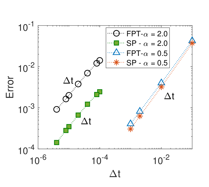
for the right side. The truncation error for this scheme is $\mathcal{O}(\Delta x)$ (see figure 2 top right panel) [196, 197]. For the special case $\alpha=2$ the central difference scheme has truncation error $\mathcal{O}(\Delta x^{2})$ (see figure 12 top right panel). For comparison, in [194] an error estimate of order $\mathcal{O}(\Delta x^{3-\alpha})$ is presented for $1<\alpha<2$ . In [198] a computational algorithm for approximating the Caputo derivative was developed, and the convergence order is $\mathcal{O}(\Delta x^{2})$ for $0<\alpha\leq 2$ . Another difference method of order two was derived in [197] for $1<\alpha\leq 2$ .

For the special case $\alpha=1$ , $\beta=0$ ,

	$\displaystyle-\frac{d}{dx}(Hf(x,t))$	$\displaystyle\approx$	$\displaystyle-\frac{2}{\pi}\displaystyle\sum_{k=1}^{i}\frac{f^{j}_{k}-f^{j}_{k-1}}{\Delta x}\frac{1}{2(i-k)+1}$		(3fhmnqce)
			$\displaystyle-\frac{2}{\pi}\displaystyle\sum_{k=i}^{I-1}\frac{f^{j}_{k}-f^{j}_{k+1}}{\Delta x}\frac{1}{2(k-i)+1}+\mathcal{O}(\Delta x^{2}),$		(3fhmnqce)

the truncation error is $\mathcal{O}(\Delta x^{2})$ (see figure 12 top left panel). To evaluate the truncation error we used the relation

\|e(x)\|_{2}=\|f(x_{i},t_{j})-f_{i}^{j}\|_{2}=\sqrt{\frac{1}{I}\displaystyle\sum_{i=1}^{I}(f(x_{i},t_{j})-f_{i}^{j})^{2}},

(3fhmnqcf)

where $f(x_{i},t_{j})$ is the exact solution and $f_{i}^{j}$ is the approximated solution of function $f(x,t)$ . For $\|e(t)\|_{2}$ this is similar and we use

\|e(t)\|_{2}=\sqrt{\frac{1}{J}\displaystyle\sum_{j=1}^{J}(f(x_{i},t_{j})-f_{i}^{j})^{2}}.

(3fhmnqcg)

The results of the error analysis for $\ell_{\alpha,\beta}(x,t)$ , survival probability and the first-passage time PDF are shown in figure 12.

Appendix D A short review of the Skorokhod theorem

The Skorokhod theorem establishes a general formula for the Laplace transform $\wp(\lambda)$ of the first-passage time PDF in the semi-infinite domain for a broad class of homogeneous random processes with independent increments and thus has a pivotal role in the theory of first-passage processes [132, 164]. For the process starting at $x=0$ with a boundary at $x=d$ ,

\wp(\lambda)=\langle e^{-\lambda t}\rangle=\int\limits_{0}^{\infty}e^{-\lambda t}\wp(t)\mathrm{d}t=1-p_{+}(\lambda,d).

(3fhmnqch)

Here the auxiliary measure $p_{+}(\lambda,x)$ is defined via its Fourier transform as

q_{+}(\lambda,k)=\int\limits_{-\infty}^{\infty}e^{\mathrm{i}kx}\frac{\partial p_{+}(\lambda,x)}{\partial x}\mathrm{d}x=\exp\left\{\int\limits_{0}^{\infty}\frac{e^{-\lambda t}}{t}\int\limits_{0}^{\infty}(e^{\mathrm{i}kx}-1)f(x,t)\mathrm{d}x\mathrm{d}t\right\},

(3fhmnqci)

where the function $f(x,t)$ is the PDF of the process, that is $\ell_{\alpha,\beta}(x,t)$ in our case. The boundary condition reads $p_{+}(\lambda,x)=0$ at $x=0$ . Below, for didactic purposes we first calculate $\wp(t)$ for Brownian motion and then proceed to symmetric ( $0<\alpha\leq 2$ and $\beta=0)$ , one-sided ( $0<\alpha<1$ and $\beta=\pm 1$ ), extremal two-sided ( $1<\alpha<2$ and $\beta=\pm 1$ ), and finally to the general case ( $0<\alpha<2$ , $\alpha\neq 1$ , and $-1<\beta<1$ ).

D.1 First passage time PDF for Brownian motion

For Brownian motion the PDF reads

f(x,t)=\frac{1}{\sqrt{4\pi K_{2}t}}\exp\left(-\frac{x^{2}}{4K_{2}t}\right).

(3fhmnqcj)

Substitution into equation (3fhmnqci) yields

$\displaystyle q_{+}(\lambda,k)$	$\displaystyle=$	$\displaystyle\exp\left\{\int\limits_{0}^{\infty}\frac{e^{-\lambda t}}{t}\int\limits_{0}^{\infty}(e^{\mathrm{i}kx}-1)\frac{e^{-x^{2}/(4K_{2}t)}}{\sqrt{4\pi K_{2}t}}\mathrm{d}x\mathrm{d}t\right\}$	(3fhmnqck)
	$\displaystyle=$	$\displaystyle\exp\left\{\int\limits_{0}^{\infty}\frac{e^{-\lambda t}}{t}\frac{1}{2}\left\{e^{-tK_{2}k^{2}}\mathrm{erfc}\left(-\mathrm{i}k\sqrt{tK_{2}}\right)-1\right\}\right\}$
	$\displaystyle=$	$\displaystyle\exp\left\{\frac{1}{2}\left[\ln{\left(\frac{\lambda}{\lambda+K_{2}k^{2}}\right)}+\ln{\left(\frac{1+\mathrm{i}k\sqrt{\frac{K_{2}}{\lambda}}}{1-\mathrm{i}k\sqrt{\frac{K_{2}}{\lambda}}}\right)}\right]\right\},$

therefore

q_{+}(\lambda,k)=\left[\frac{\lambda}{\lambda+K_{2}k^{2}}\left(\frac{1+\mathrm{i}k\sqrt{\frac{K_{2}}{\lambda}}}{1-\mathrm{i}k\sqrt{\frac{K_{2}}{\lambda}}}\right)\right]^{1/2}.

(3fhmnqcl)

Now, we use the relation

\frac{1}{1-\mathrm{i}k\sqrt{K_{2}/\lambda}}=\frac{1+\mathrm{i}k\sqrt{K_{2}/\lambda}}{1+K_{2}k^{2}/\lambda}

(3fhmnqcm)

to get to

q_{+}(\lambda,k)=\frac{\lambda}{\lambda+K_{2}k^{2}}+\frac{\mathrm{i}k\sqrt{K_{2}\lambda}}{\lambda+K_{2}k^{2}}.

(3fhmnqcn)

After an inverse Fourier transform according to equation (3fhmnqci) we arrive at

\frac{d}{dx}p_{+}(\lambda,x)=\frac{1}{2\pi}\int\limits_{-\infty}^{\infty}e^{-\mathrm{i}kx}q_{+}(\lambda,k)\mathrm{d}k=\frac{1}{2\pi}\int\limits_{-\infty}^{\infty}e^{-\mathrm{i}kx}\left(\frac{\lambda}{\lambda+K_{2}k^{2}}+\frac{\mathrm{i}k\sqrt{K_{2}\lambda}}{\lambda+K_{2}k^{2}}\right)\mathrm{d}k.

(3fhmnqco)

For the first integral we have

\frac{1}{2\pi}\int\limits_{-\infty}^{\infty}e^{-\mathrm{i}kx}\left(\frac{\lambda}{\lambda+K_{2}k^{2}}\right)\mathrm{d}k=\frac{\lambda}{2\pi K_{2}}\int\limits_{-\infty}^{\infty}\frac{e^{-\mathrm{i}kx}}{\left(k-\mathrm{i}\sqrt{\frac{\lambda}{K_{2}}}\right)\left(k+\mathrm{i}\sqrt{\frac{\lambda}{K_{2}}}\right)}\mathrm{d}k.

(3fhmnqcp)

With the residue theorem,

\frac{\lambda}{2\pi K_{2}}\int\limits_{-\infty}^{\infty}\frac{e^{-\mathrm{i}kx}}{\left(k-\mathrm{i}\sqrt{\frac{\lambda}{K_{2}}}\right)\left(k+\mathrm{i}\sqrt{\frac{\lambda}{K_{2}}}\right)}\mathrm{d}k=\frac{1}{2}\sqrt{\frac{\lambda}{K_{2}}}\exp{\left(-\sqrt{\frac{\lambda}{K_{2}}}x\right)},

(3fhmnqcq)

For the second integral, we write

\frac{1}{2\pi}\int\limits_{-\infty}^{\infty}e^{-\mathrm{i}kx}\left(\frac{\mathrm{i}k\sqrt{K_{2}\lambda}}{\lambda+K_{2}k^{2}}\right)\mathrm{d}k=\frac{\mathrm{i}}{2\pi}\sqrt{\frac{\lambda}{K_{2}}}\int\limits_{-\infty}^{\infty}\frac{k\rme^{-\mathrm{i}kx}}{\left(k-\mathrm{i}\sqrt{\frac{\lambda}{K_{2}}}\right)\left(k+\mathrm{i}\sqrt{\frac{\lambda}{K_{2}}}\right)}\mathrm{d}k.

(3fhmnqcr)

Again, with the residue theorem,

\frac{\mathrm{i}}{2\pi}\sqrt{\frac{\lambda}{K_{2}}}\int\limits_{-\infty}^{\infty}\frac{k\rme^{-\mathrm{i}kx}}{(k-\mathrm{i}\sqrt{\frac{\lambda}{K_{2}}})(k+\mathrm{i}\sqrt{\frac{\lambda}{K_{2}}})}\mathrm{d}k=\frac{1}{2}\sqrt{\frac{\lambda}{K_{2}}}\exp{\left(-\sqrt{\frac{\lambda}{K_{2}}}x\right)}.

(3fhmnqcs)

Therefore, by substitution of equations (3fhmnqcq) and (3fhmnqcs) into equation (3fhmnqco) we obtain ( $x>0$ )

\frac{d}{dx}p_{+}(\lambda,x)=\frac{1}{2\pi}\int\limits_{-\infty}^{\infty}e^{-\mathrm{i}kx}\hat{q}_{+}(\lambda,k)\mathrm{d}k=\sqrt{\frac{\lambda}{K_{2}}}\exp{\left(-\sqrt{\frac{\lambda}{K_{2}}}x\right)}.

(3fhmnqct)

Using the boundary condition we get

p_{+}(\lambda,x)=\sqrt{\frac{\lambda}{K_{2}}}\int\limits_{0}^{x}\exp{\left(-\sqrt{\frac{\lambda}{K_{2}}}x\right)}\mathrm{d}x=1-\exp{\left(-\sqrt{\frac{\lambda}{K_{2}}}x\right)},

(3fhmnqcu)

and thus with the help of equation (3fhmnqch),

\wp(\lambda)=\exp\left(-\sqrt{\frac{\lambda}{K_{2}}}d\right),

(3fhmnqcv)

Finally, by inverse Laplace transform we get

\wp(t)=\frac{d}{\sqrt{4\pi K_{2}t^{3}}}\exp\left(-\frac{d^{2}}{4K_{2}t}\right).

(3fhmnqcw)

This is the famous Lévy-Smirnov law representing a well-known result of Brownian motion [165]. This derivation is, of course, overly complicated for the Gaussian case, but the same procedure can be applied to the general case of an asymmetric Lévy stable law, as we now show.

D.2 First passage time PDF for symmetric $\alpha$ -stable processes

Due to the symmetry of the PDF the function $\ln q_{+}(k,\lambda)$ , equation (3fhmnqci), can be written as

\ln{q_{+}(k,\lambda)}=A(\lambda,k)+\mathrm{i}B(\lambda,k),

(3fhmnqcx)

where

A(\lambda,k)=\int\limits_{0}^{\infty}\frac{e^{-\lambda t}}{t}\int\limits_{0}^{\infty}(\cos{(kx)}-1)\ell_{\alpha,0}(x,t)\,\mathrm{d}x\mathrm{d}t=\frac{1}{2}\ln{\frac{\lambda}{\lambda+K_{\alpha}|k|^{\alpha}}},

(3fhmnqcy)

and

B(\lambda,k)=\int\limits_{0}^{\infty}\frac{e^{-\lambda t}}{t}\int\limits_{0}^{\infty}\sin{(kx)}\ell_{\alpha,0}(x,t)\mathrm{d}x\mathrm{d}t.

(3fhmnqcz)

To find $B(\lambda,k)$ at small $\lambda$ the self-similar property of the $\alpha$ -stable process comes in useful,

\ell_{\alpha,0}(x,t)=\frac{1}{(K_{\alpha}t)^{1/\alpha}}\ell_{\alpha,0}\left(\frac{x}{(K_{\alpha}t)^{1/\alpha}},1\right),

(3fhmnqda)

where

\ell_{\alpha,0}(y,1)=\ell_{\alpha,0}(-y,1)=\frac{1}{\pi}\int\limits_{0}^{\infty}\cos{(ky)}e^{-|k|^{\alpha}}\mathrm{d}k.

(3fhmnqdb)

When $\lambda$ tends to zero, from equation (3fhmnqcz) we get

$\displaystyle B(\lambda,k)$	$\displaystyle=$	$\displaystyle\int\limits_{0}^{\infty}\frac{e^{-\lambda t}}{t}\int\limits_{0}^{\infty}\sin{(kx)}\frac{1}{(K_{\alpha}t)^{1/\alpha}}\ell_{\alpha,0}\left(x/(K_{\alpha}t)^{1/\alpha},1\right)\,\mathrm{d}x\mathrm{d}t$	(3fhmnqdc)
	$\displaystyle\approx$	$\displaystyle\int\limits_{0}^{\infty}\frac{1}{t}\int\limits_{0}^{\infty}\sin{(ky(K_{\alpha}t)^{1/\alpha})}\ell_{\alpha,0}(y,1)\mathrm{d}y\mathrm{d}t$
	$\displaystyle=$	$\displaystyle\alpha\int\limits_{0}^{\infty}\ell_{\alpha,0}(y,1)\int\limits_{0}^{\infty}\frac{\sin{(kys)}}{s}\mathrm{d}s\mathrm{d}y=\frac{\alpha\pi}{4}\mathrm{sgn}(k).$

By substitution of equations (3fhmnqcy) and (3fhmnqdc) into equation (3fhmnqcx) we get

q_{+}(\lambda,k)\approx\frac{\sqrt{\lambda}}{\sqrt{K_{\alpha}}|k|^{\alpha/2}}e^{\mathrm{i}\mathrm{sgn}(k)\alpha\pi/4},\quad\lambda\to 0.

(3fhmnqdd)

Then the inverse Fourier transform of the above equation renders

\frac{d}{dx}p_{+}(\lambda,x)=\frac{1}{2\pi}\int\limits_{-\infty}^{\infty}e^{-\mathrm{i}kx}\hat{q}_{+}(\lambda,k)\mathrm{d}k=\frac{\sqrt{\lambda}}{\sqrt{K_{\alpha}}\Gamma(\alpha/2)}x^{-1+\alpha/2},

(3fhmnqde)

and, after applying the boundary condition,

p_{+}(\lambda,x)=\frac{2\sqrt{\lambda}}{\alpha\sqrt{K_{\alpha}}\Gamma(\alpha/2)}x^{\alpha/2}.

(3fhmnqdf)

Recalling equation (3fhmnqch),

\wp(\lambda)\approx 1-\frac{2d^{\alpha/2}}{\alpha\sqrt{K_{\alpha}}\Gamma(\alpha/2)}\lambda^{1/2}.

(3fhmnqdg)

Now, with the help of the Tauberian theorem [165] (Chapter XIII, section 5) we find that the small- $\lambda$ asymptotic of the Laplace transform

\psi(\lambda)\approx 1-b_{2}\lambda^{\mu},\quad b_{2}=b_{1}\Gamma(1-\mu)/\mu,\quad\lambda\to 0

(3fhmnqdh)

corresponds to the long-time asymptotic of the PDF ([199], chapter 3)

\psi(t)\sim b_{1}t^{-1-\mu},\quad 0<\mu<1,\quad b_{1}>0.

(3fhmnqdi)

Therefore, the long-time asymptotic of the first-passage time PDF for symmetric $\alpha$ -stable process has the form [125]

\wp(t)\approx\frac{d^{\alpha/2}}{\alpha\sqrt{\pi K_{\alpha}}\Gamma{(\alpha/2)}}t^{-3/2}.

(3fhmnqdj)

D.3 First passage time PDF for one-sided $\alpha$ -stable processes, $0<\alpha<1$ and $\beta=1$

Due to the monotonic growth of the process in this case there exists a simple relation between the cumulative probabilities of the first-passage time and the $\alpha$ -stable process itself, see, e.g., [168]. However, for a didactic purpose in this Appendix we obtain the result by the use of Skorokhod’s method. Since for one-sided $\alpha$ -stable processes with $0<\alpha<1$ and $\beta=1$ the PDF $\ell_{\alpha,1}(x,t)$ vanishes for $x<0$ , we get

	$\displaystyle\int\limits_{0}^{\infty}\left(e^{\mathrm{i}kx}-1\right)\ell_{\alpha,1}(x,t)\mathrm{d}x$	$\displaystyle=$	$\displaystyle\int\limits_{-\infty}^{\infty}\left(e^{\mathrm{i}kx}-1\right)\ell_{\alpha,1}(x,t)\mathrm{d}x$		(3fhmnqdk)
		$\displaystyle=$	$\displaystyle\exp{\left[-tK_{\alpha}\|k\|^{\alpha}\left(1-\mathrm{i}\mathrm{sgn}(k)\tan(\alpha\pi/2)\right)\right]}-1.$		(3fhmnqdk)

After plugging this into equation (3fhmnqci),

q_{+}(\lambda,k)=\exp\left\{\int\limits_{0}^{\infty}\frac{e^{-\lambda t}}{t}\left(\exp{\left[-tK_{\alpha}|k|^{\alpha}\left(1-\mathrm{i}\mathrm{sgn}(k)\tan(\alpha\pi/2)\right)\right]}-1\right)\mathrm{d}t\right\}.

(3fhmnqdl)

Then

q_{+}(\lambda,k)=\exp{\left\{\ln{\left(\frac{\lambda}{\lambda+\zeta}\right)}\right\}}=\frac{\lambda}{\lambda+\zeta},

(3fhmnqdm)

where

\zeta=K_{\alpha}|k|^{\alpha}\left(1-\mathrm{i}\mathrm{sgn}(k)\tan{\frac{\pi\alpha}{2}}\right)=\frac{K_{\alpha}}{\cos{(\alpha\pi/2)}}(-\mathrm{i}k)^{\alpha}.

(3fhmnqdn)

Therefore, $\partial p_{+}(\lambda,x)/\partial x$ follows from result (3fhmnqdm) by inverse Fourier transform,

\frac{d}{dx}p_{+}(\lambda,x)=\frac{1}{2\pi}\int\limits_{-\infty}^{\infty}e^{-\mathrm{i}kx}q_{+}(\lambda,k)\mathrm{d}k=\frac{1}{2\pi}\int\limits_{-\infty}^{\infty}e^{-\mathrm{i}kx}\left(\frac{\lambda}{(-\mathrm{i}k)^{\alpha}\frac{K_{\alpha}}{\cos{(\alpha\pi/2)}}+\lambda}\right)\mathrm{d}k.

(3fhmnqdo)

Defining $s=-\mathrm{i}k$ , we have

\frac{\mathrm{d}}{\mathrm{d}x}p_{+}(\lambda,x)=\frac{1}{2\pi\mathrm{i}}\int\limits_{-\mathrm{i}\infty}^{\mathrm{i}\infty}e^{sx}\frac{\lambda}{s^{\alpha}K_{\alpha}/[\cos(\alpha\pi/2)]+\lambda}\mathrm{d}s.

(3fhmnqdp)

Recalling relation (3fhmnqgc) we obtain

\frac{\mathrm{d}}{\mathrm{d}x}p_{+}(\lambda,x)=-\frac{\mathrm{d}}{\mathrm{d}x}E_{\alpha}\left(-\frac{\lambda\cos{(\alpha\pi/2)}}{K_{\alpha}}x^{\alpha}\right),

(3fhmnqdq)

where $E_{\alpha}(z)=\sum_{n=0}^{\infty}z^{n}/\Gamma(1+\alpha n)$ is the Mittag-Leffler function, see [138, 167] and E. With the boundary condition $p_{+}(\lambda,x\leq 0)=0$ we get

p_{+}(\lambda,x)=1-E_{\alpha}\left(-\frac{\lambda\cos{(\alpha\pi/2)}}{K_{\alpha}}x^{\alpha}\right).

(3fhmnqdr)

Thus, for the Laplace transform of the first-passage time PDF $\wp(\lambda)=1-p_{+}(\lambda,d)$ we have

\wp(\lambda)=E_{\alpha}(-\lambda\cos(\alpha\pi/2)d^{\alpha}/K_{\alpha}).

(3fhmnqds)

The Laplace inversion is then immediately accomplished in terms of the Wright function (see equation (3fhmnqgj)) for $0<\alpha<1$ [125],

\wp(t)=\frac{K_{\alpha}}{\cos(\alpha\pi/2)d^{\alpha}}M_{\alpha}\left(\frac{K_{\alpha}t}{\cos(\alpha\pi/2)d^{\alpha}}\right).

(3fhmnqdt)

By using relation (3fhmnqgl) we make sure that $\wp(t)$ is normalised,

\int\limits_{0}^{\infty}\wp(t)\mathrm{d}t=\int\limits_{0}^{\infty}\frac{K_{\alpha}}{\cos(\alpha\pi/2)d^{\alpha}}M_{\alpha}\left(\frac{K_{\alpha}t}{\cos(\alpha\pi/2)d^{\alpha}}\right)\mathrm{d}t=1.

(3fhmnqdu)

This can be also shown by taking the integral form (3fhmnqgh) of the $M$ -function. By changing the order of integration we get

$\displaystyle\int\limits_{0}^{\infty}\wp(t)\mathrm{d}t$	$\displaystyle=$	$\displaystyle\int\limits_{0}^{\infty}\frac{K_{\alpha}}{\cos(\alpha\pi/2)d^{\alpha}}\frac{1}{2\pi\mathrm{i}}\int\limits_{\mathrm{Ha}}\exp{\left(\sigma-\frac{K_{\alpha}t}{\cos(\alpha\pi/2)d^{\alpha}}\sigma^{\alpha}\right)}\frac{\mathrm{d}\sigma}{\sigma^{1-\alpha}}\mathrm{d}t$	(3fhmnqdv)
	$\displaystyle=$	$\displaystyle\frac{1}{2\pi\mathrm{i}}\int\limits_{\mathrm{Ha}}\sigma^{\alpha-1}\rme^{\sigma}\frac{K_{\alpha}}{\cos(\alpha\pi/2)d^{\alpha}}\int\limits_{0}^{\infty}\exp\left(-\frac{K_{\alpha}\sigma^{\alpha}}{\cos(\alpha\pi/2)d^{\alpha}}t\right)\mathrm{d}t\mathrm{d}\sigma$
	$\displaystyle=$	$\displaystyle\frac{1}{2\pi\mathrm{i}}\int\limits_{\mathrm{Ha}}\sigma^{-1}\rme^{\sigma}\mathrm{d}\sigma=1,$

where Ha denotes the Hankel path, and in the last step we made use of equation (3fhmnqga).

D.4 First passage time PDF for extremal two-sided $\alpha$ -stable process, $1<\alpha<2$ and $\beta=-1$

To apply the Skorokhod theorem we need to calculate the following integral

\int\limits_{0}^{\infty}\left(e^{\mathrm{i}kx}-1\right)\ell_{\alpha,-1}(x,t)\mathrm{d}x.

(3fhmnqdw)

To this end we use the Laplace transform of $\alpha$ -stable processes with $1<\alpha\leq 2$ and $\beta_{B}=-1$ , which is derived in [154] (page 169, equation (2.10.9)) in dimensionless B-form with $K_{\alpha}^{B}=1$ and $t=1$ ,

\frac{1}{\alpha}E_{1/\alpha}\left(-s\right)=\int\limits_{0}^{\infty}e^{-sx}\ell_{\alpha,-1}^{B}(x,1)\mathrm{d}x.

(3fhmnqdx)

In dimensional variables this equation reads

\frac{1}{\alpha}E_{1/\alpha}\left(-s\left(K_{\alpha}^{B}t\right)^{1/\alpha}\right)=\int\limits_{0}^{\infty}e^{-sx}\ell_{\alpha,-1}^{B}(x,t)\mathrm{d}x.

(3fhmnqdy)

With the help of equation (3fhmnqaz) we have in the A-form

\int\limits_{0}^{\infty}e^{-sx}\ell_{\alpha,-1}^{A}(x,t)\mathrm{d}x=\frac{1}{\alpha}E_{1/\alpha}\left(-s\left(\frac{K_{\alpha}^{A}t}{|\cos{(\alpha\pi/2)}|}\right)^{1/\alpha}\right).

(3fhmnqdz)

Now we go back to equation (3fhmnqdw) which can be written as (we again omit the index $A$ in what follows)

\int\limits_{0}^{\infty}e^{-sx}\ell_{\alpha,-1}(x,t)|_{s=-\mathrm{i}k}\mathrm{d}x-\int\limits_{0}^{\infty}e^{-sx}\ell_{\alpha,-1}(x,t)|_{s=0}\mathrm{d}x.

(3fhmnqea)

Using equation (3fhmnqdz) we find

\int\limits_{0}^{\infty}\left(e^{\mathrm{i}kx}-1\right)\ell_{\alpha,-1}(x,t)\mathrm{d}x=\frac{1}{\alpha}\left[E_{1/\alpha}\left(\mathrm{i}k\left(\frac{K_{\alpha}t}{|\cos{(\alpha\pi/2)}|}\right)^{1/\alpha}\right)-1\right],

(3fhmnqeb)

and after plugging this expression into equation (3fhmnqci),

q_{+}(\lambda,k)=\exp\left\{\frac{1}{\alpha}\int\limits_{0}^{\infty}\frac{e^{-\lambda t}}{t}\left[E_{1/\alpha}\left(\mathrm{i}k\left(\frac{K_{\alpha}t}{|\cos{(\alpha\pi/2)}|}\right)^{1/\alpha}\right)-1\right]\mathrm{d}t\right\}.

(3fhmnqec)

To calculate expression (3fhmnqec) we first find

	$\displaystyle\frac{\partial}{\partial\lambda}\ln{q_{+}(\lambda,k)}$	$\displaystyle=$	$\displaystyle-\frac{1}{\alpha}\int\limits_{0}^{\infty}\rme^{-\lambda t}\left[E_{1/\alpha}\left(\mathrm{i}k\left(\frac{K_{\alpha}t}{\|\cos{(\alpha\pi/2)}\|}\right)^{1/\alpha}\right)-1\right]\mathrm{d}t$		(3fhmnqed)
		$\displaystyle=$	$\displaystyle\frac{1}{\alpha\lambda}\left[1-\frac{\lambda^{1/\alpha}}{\lambda^{1/\alpha}-\mathrm{i}k\left(\frac{K_{\alpha}}{\|\cos(\alpha\pi/2)\|}\right)^{1/\alpha}}\right],$		(3fhmnqed)

where we employ the Laplace transform (3fhmnqgb) of the Mittag-Leffler function. By taking the indefinite integral over $\lambda$ we obtain

q_{+}(\lambda,k)=\frac{\lambda^{1/\alpha}}{\lambda^{1/\alpha}-\mathrm{i}k\left(\frac{K_{\alpha}}{|\cos(\alpha\pi/2)|}\right)^{1/\alpha}},

(3fhmnqee)

and then from equation (3fhmnqee), by inverse Fourier transform,

	$\displaystyle\frac{d}{dx}p_{+}(\lambda,x)$	$\displaystyle=$	$\displaystyle\frac{1}{2\pi}\int\limits_{-\infty}^{\infty}e^{-\mathrm{i}kx}q_{+}(\lambda,k)\mathrm{d}k$		(3fhmnqef)
		$\displaystyle=$	$\displaystyle\left(\frac{\|\cos{(\alpha\pi/2)}\|}{K_{\alpha}}\right)^{1/\alpha}\lambda^{1/\alpha}\exp{\left[-\left(\frac{\|\cos{(\alpha\pi/2)}\|}{K_{\alpha}}\right)^{1/\alpha}x\lambda^{1/\alpha}\right]}.$		(3fhmnqef)

With the boundary condition $p_{+}(\lambda,x=0)=0$ we get

p_{+}(\lambda,x)=1-\exp{\left[-\left(\frac{|\cos{(\alpha\pi/2)}|}{K_{\alpha}}\right)^{1/\alpha}x\lambda^{1/\alpha}\right]}.

(3fhmnqeg)

Thus, for the Laplace transform $\wp(\lambda)$ we obtain

\wp(\lambda)=1-p_{+}(\lambda,d)=\exp{\left[-d\left(\frac{|\cos{(\alpha\pi/2)}|}{K_{\alpha}}\right)^{1/\alpha}\lambda^{1/\alpha}\right]},

(3fhmnqeh)

which is of a stretched exponential form. Recalling now the Laplace transform pair (3fhmnqgk) for the $M$ -function, we finally arrive at the first-passage time PDF for the extremal $\alpha$ -stable process with $1<\alpha\leq 2$ and $\beta=-1$ ,

\wp(t)=\frac{t^{-1-1/\alpha}d}{\alpha\left(\frac{K_{\alpha}}{|\cos{(\alpha\pi/2)}|}\right)^{1/\alpha}}M_{1/\alpha}\left(d\left(\frac{K_{\alpha}t}{|\cos{(\alpha\pi/2)}|}\right)^{-1/\alpha}\right).

(3fhmnqei)

Let us show the normalisation of this function. By using the integral form (3fhmnqgh) of the $M$ -function and changing the order of integration we have

$\displaystyle\int\limits_{0}^{\infty}\wp(t)\mathrm{d}t$	$\displaystyle=$	$\displaystyle\frac{d}{\alpha\left(\frac{K_{\alpha}}{\|\cos(\alpha\pi/2)\|}\right)^{1/\alpha}}\int\limits_{0}^{\infty}t^{-1-1/\alpha}M_{1/\alpha}\left(d\left(\frac{K_{\alpha}t}{\|\cos{(\alpha\pi/2)}\|}\right)^{-1/\alpha}\right)\mathrm{d}t$	(3fhmnqej)
	$\displaystyle=$	$\displaystyle\int\limits_{0}^{\infty}\frac{t^{-1}}{\alpha}\left[\frac{K_{\alpha}t}{d^{\alpha}\|\cos{(\alpha\pi/2)}\|}\right]^{-1/\alpha}$
		$\displaystyle\times\frac{1}{2\pi i}\int\limits_{\mathrm{Ha}}\exp{\left(\sigma-\left[\frac{K_{\alpha}t}{d^{\alpha}\|\cos{(\alpha\pi/2)}\|}\right]^{-1/\alpha}\sigma^{1/\alpha}\right)}\frac{\mathrm{d}\sigma}{\sigma^{1-1/\alpha}}\mathrm{d}t$
	$\displaystyle=$	$\displaystyle\frac{1}{2\pi i}\int\limits_{\mathrm{Ha}}\rme^{\sigma}\sigma^{1/\alpha-1}\int\limits_{0}^{\infty}\frac{t^{-1}}{\alpha}\left[\frac{K_{\alpha}t}{d^{\alpha}\|\cos{(\alpha\pi/2)}\|}\right]^{-1/\alpha}$
		$\displaystyle\times\exp{\left(-\left[\frac{K_{\alpha}}{d^{\alpha}\|\cos{(\alpha\pi/2)}\|\sigma}\right]^{-1/\alpha}t^{-1/\alpha}\right)}\mathrm{d}t\mathrm{d}\sigma.$

By change of variable $u=\left[{K_{\alpha}/d^{\alpha}|\cos{(\alpha\pi/2)}|\sigma}\right]^{-1/\alpha}t^{-1/\alpha}$ , performing the inner integral and using the Hankel formula (3fhmnqga) for the Gamma function we obtain the necessary normalisation condition. Now, if we employ the series expansion (3fhmnqgg) for the $M$ -function, from equation (3fhmnqei) we arrive at a series which corresponds to that in equation (2.25) of [172]. Note that in our case the additional factor $K_{\alpha}/|\cos(\alpha\pi/2)|$ appears due to a different starting form for the characteristic function of the $\alpha$ -stable process.

D.5 First passage time PDF for extremal two-sided $\alpha$ -stable processes, $1<\alpha<2$ , $\beta=1$

Similar to above, at first we obtain the Laplace transform of the $\alpha$ -stable PDF with $1<\alpha\leq 2$ and $\beta=1$ . We write

\int\limits_{0}^{\infty}f(u)\mathrm{d}u=\int\limits_{-\infty}^{\infty}f(u)\mathrm{d}u-\int\limits_{-\infty}^{0}f(u)\mathrm{d}u,

(3fhmnqek)

and then use the property $\ell_{\alpha,\beta}(x,t)=\ell_{\alpha,-\beta}(-x,t)$ to get

\int\limits_{0}^{\infty}e^{\mathrm{i}kx}\ell_{\alpha,1}(x,t)\mathrm{d}x=\int\limits_{-\infty}^{\infty}e^{\mathrm{i}kx}\ell_{\alpha,1}(x,t)\mathrm{d}x-\int\limits_{-\infty}^{0}e^{\mathrm{i}kx}\ell_{\alpha,-1}(-x,t)\mathrm{d}x.

(3fhmnqel)

The second integral on the right side can be written as

\int\limits_{-\infty}^{0}e^{\mathrm{i}kx}\ell_{\alpha,-1}(-x,t)\mathrm{d}x=\int\limits_{0}^{\infty}e^{-\mathrm{i}kx}\ell_{\alpha,-1}(x,t)\mathrm{d}x.

(3fhmnqem)

To take the first integral on the right hand side of equation (3fhmnqel) we use the characteristic function in the A-form. To take the second integral (3fhmnqem) we employ the Laplace transform of the PDF with $1<\alpha<2$ and $\beta=-1$ given by equation (3fhmnqdz) with $s=\mathrm{i}k$ . Thus, relation (3fhmnqel) in the A-form has the shape

\int\limits_{0}^{\infty}e^{\mathrm{i}kx}\ell_{\alpha,1}^{A}(x,t)\mathrm{d}x=\exp{\left(\frac{(-\mathrm{i}k)^{\alpha}K_{\alpha}^{A}t}{|\cos{(\alpha\pi/2)}|}\right)}-\frac{1}{\alpha}E_{1/\alpha}\left(\left[\frac{(-\mathrm{i}k)^{\alpha}K_{\alpha}^{A}t}{|\cos{(\alpha\pi/2)}|}\right]^{1/\alpha}\right).

(3fhmnqen)

With the help of equation (3fhmnqen) we write (again the index $A$ is omitted in what follows)

	$\displaystyle\int\limits_{0}^{\infty}\left(e^{\mathrm{i}kx}-1\right)\ell_{\alpha,1}(x,t)\mathrm{d}x$	$\displaystyle=$	$\displaystyle\int\limits_{0}^{\infty}e^{-sx}\ell_{\alpha,1}(x,t)\|_{s=-\mathrm{i}k}\mathrm{d}x-\int\limits_{0}^{\infty}e^{-sx}\ell_{\alpha,1}(x,t)\|_{s=0}\mathrm{d}x$		(3fhmnqeo)
			$\displaystyle\hskip-79.6678pt=\left[\exp{\left(\frac{(-\mathrm{i}k)^{\alpha}K_{\alpha}t}{\|\cos{(\alpha\pi/2)}\|}\right)}-\frac{1}{\alpha}E_{1/\alpha}\left(\left[\frac{(-\mathrm{i}k)^{\alpha}K_{\alpha}t}{\|\cos{(\alpha\pi/2)}\|}\right]^{1/\alpha}\right)-1+\frac{1}{\alpha}\right].$		(3fhmnqeo)

By substituting this expression into equation (3fhmnqci) we get

	$\displaystyle\ln{q_{+}(\lambda,k)}$	$\displaystyle=$	$\displaystyle\int\limits_{0}^{\infty}\frac{e^{-\lambda t}}{t}\left[\exp{\left(\frac{(-\mathrm{i}k)^{\alpha}K_{\alpha}t}{\|\cos{(\alpha\pi/2)}\|}\right)}\right.$		(3fhmnqep)
			$\displaystyle\left.-\frac{1}{\alpha}E_{1/\alpha}\left(\left[\frac{(-\mathrm{i}k)^{\alpha}K_{\alpha}t}{\|\cos{(\alpha\pi/2)}\|}\right]^{1/\alpha}\right)-1+\frac{1}{\alpha}\right]\mathrm{d}t.$		(3fhmnqep)

The derivative with respect to $\lambda$ reads

$\displaystyle\frac{\partial}{\partial\lambda}\ln{q_{+}(\lambda,k)}$	$\displaystyle=$	$\displaystyle-\int\limits_{0}^{\infty}\rme^{-\lambda t}\left[\exp{\left(\frac{(-\mathrm{i}k)^{\alpha}K_{\alpha}t}{\|\cos{(\alpha\pi/2)}\|}\right)}\right.$	(3fhmnqeq)
		$\displaystyle\left.-\frac{1}{\alpha}E_{1/\alpha}\left(\left[\frac{(-\mathrm{i}k)^{\alpha}K_{\alpha}t}{\|\cos{(\alpha\pi/2)}\|}\right]^{1/\alpha}\right)-1+\frac{1}{\alpha}\right]\mathrm{d}t$
	$\displaystyle=$	$\displaystyle-\frac{1}{\lambda-\frac{(-\mathrm{i}k)^{\alpha}K_{\alpha}}{\|\cos{(\alpha\pi/2)}\|}}+\frac{1}{\alpha}\frac{\lambda^{1/\alpha-1}}{\lambda^{1/\alpha}-\left(\frac{(-\mathrm{i}k)^{\alpha}K_{\alpha}}{\|\cos{(\alpha\pi/2)}\|}\right)^{1/\alpha}}+\left(1-\frac{1}{\alpha}\right)\frac{1}{\lambda},$

where for the second term we employ the Laplace transform (3fhmnqgb) of the Mittag-Leffler function. By taking the indefinite integral over $\lambda$ we obtain

q_{+}(\lambda,k)=\frac{\lambda^{1-1/\alpha}\left(\lambda^{1/\alpha}-\left(\frac{(-\mathrm{i}k)^{\alpha}K_{\alpha}}{|\cos{(\alpha\pi/2)}|}\right)^{1/\alpha}\right)}{\lambda-\frac{(-\mathrm{i}k)^{\alpha}K_{\alpha}}{|\cos{(\alpha\pi/2)}|}}.

(3fhmnqer)

Then, $dp_{+}(\lambda,x)/dx$ follows from equation (3fhmnqer) by inverse Fourier transform,

\frac{d}{dx}p_{+}(\lambda,x)=\frac{1}{2\pi}\int\limits_{-\infty}^{\infty}e^{-\mathrm{i}kx}\left(\frac{1+\mathrm{i}k\left(\frac{K_{\alpha}}{|\cos{(\alpha\pi/2)}|\lambda}\right)^{1/\alpha}}{1-(-\mathrm{i}k)^{\alpha}\frac{K_{\alpha}}{|\cos{(\alpha\pi/2)}|\lambda}}\right)\mathrm{d}k.

(3fhmnqes)

By defining $s=-\mathrm{i}k$ we have

	$\displaystyle\frac{\mathrm{d}}{\mathrm{d}x}p_{+}(\lambda,x)$	$\displaystyle=$	$\displaystyle\frac{1}{2\pi\mathrm{i}}\int\limits_{-i\infty}^{i\infty}e^{sx}\frac{1-s\left(\frac{K_{\alpha}}{\|\cos{(\alpha\pi/2)}\|\lambda}\right)^{1/\alpha}}{1-s^{\alpha}\frac{K_{\alpha}}{\|\cos{(\alpha\pi/2)}\|\lambda}}\mathrm{d}s$		(3fhmnqet)
		$\displaystyle=$	$\displaystyle\frac{1}{2\pi\mathrm{i}}\int\limits_{-\mathrm{i}\infty}^{\mathrm{i}\infty}e^{sx}\frac{1}{1-s^{\alpha}\frac{K_{\alpha}}{\|\cos{(\alpha\pi/2)}\|\lambda}}\mathrm{d}s-\frac{1}{2\pi\mathrm{i}}\int\limits_{-\mathrm{i}\infty}^{\mathrm{i}\infty}e^{sx}\frac{s\left(\frac{K_{\alpha}}{\|\cos{(\alpha\pi/2)}\|\lambda}\right)^{1/\alpha}}{1-s^{\alpha}\frac{K_{\alpha}}{\|\cos{(\alpha\pi/2)}\|\lambda}}\mathrm{d}s.$		(3fhmnqet)

Using the properties of the Mittag-Leffler function, equations (3fhmnqgc) and (3fhmnqgd) we can write

	$\displaystyle\frac{\mathrm{d}}{\mathrm{d}x}p_{+}(\lambda,x)$	$\displaystyle=$	$\displaystyle-\frac{d}{dx}E_{\alpha}\left(\frac{\|\cos{(\alpha\pi/2)}\|\lambda x^{\alpha}}{K_{\alpha}}\right)$		(3fhmnqeu)
			$\displaystyle+\left(\frac{K_{\alpha}}{\|\cos{(\alpha\pi/2)}\|\lambda}\right)^{1/\alpha}\frac{\mathrm{d}^{2}}{\mathrm{d}x^{2}}E_{\alpha}\left(\frac{\|\cos{(\alpha\pi/2)}\|\lambda x^{\alpha}}{K_{\alpha}}\right),$		(3fhmnqeu)

and with the boundary condition $p_{+}(\lambda,x=0)=0$ we get

	$\displaystyle p_{+}(\lambda,x)$	$\displaystyle=$	$\displaystyle 1-E_{\alpha}\left(\frac{\|\cos{(\alpha\pi/2)}\|\lambda x^{\alpha}}{K_{\alpha}}\right)$		(3fhmnqev)
			$\displaystyle+\left(\frac{K_{\alpha}}{\|\cos{(\alpha\pi/2)}\|\lambda}\right)^{1/\alpha}\frac{\mathrm{d}}{\mathrm{d}x}E_{\alpha}\left(\frac{\|\cos{(\alpha\pi/2)}\|\lambda x^{\alpha}}{K_{\alpha}}\right).$		(3fhmnqev)

Thus, for the Laplace transform $\wp(\lambda)=1-p_{+}(\lambda,d)$ we obtain

\wp(\lambda)=E_{\alpha}\left(\frac{\lambda|\cos{(\alpha\pi/2)}|}{K_{\alpha}}d^{\alpha}\right)-\left(\frac{\lambda|\cos{(\alpha\pi/2)}|}{K_{\alpha}}\right)^{-1/\alpha}\frac{\mathrm{d}}{\mathrm{d}d}E_{\alpha}\left(\frac{\lambda|\cos{(\alpha\pi/2)}|}{K_{\alpha}}d^{\alpha}\right).

(3fhmnqew)

By applying the inverse Laplace transform with respect to $\lambda$ and using the series representation (3fhmnqfy) of the Mittag-Leffler function for the first term on the right side of equation (3fhmnqew) we have

$\displaystyle\frac{1}{2\pi\mathrm{i}}\int\limits_{\mathrm{Ha}}e^{\lambda t}E_{\alpha}\left(\frac{\lambda\|\cos{(\alpha\pi/2)}\|}{K_{\alpha}}d^{\alpha}\right)\mathrm{d}\lambda$	$\displaystyle=$	$\displaystyle\frac{1}{2\pi\mathrm{i}}\int\limits_{\mathrm{Ha}}e^{\lambda t}\displaystyle\sum_{n=0}^{\infty}\frac{\left(\frac{\lambda\|\cos{(\alpha\pi/2)}\|}{K_{\alpha}}d^{\alpha}\right)^{n}}{\Gamma(\alpha n+1)}\mathrm{d}\lambda$	(3fhmnqex)
		$\displaystyle\hskip-62.59596pt=\displaystyle\sum_{n=0}^{\infty}\frac{\left(\frac{\|\cos{(\alpha\pi/2)}\|}{K_{\alpha}}d^{\alpha}\right)^{n}}{\Gamma(\alpha n+1)}\frac{1}{2\pi i}\int\limits_{\mathrm{Ha}}e^{\lambda t}\lambda^{n}\mathrm{d}\lambda$
		$\displaystyle\hskip-62.59596pt=\displaystyle\sum_{n=0}^{\infty}\frac{\left(\frac{\|\cos{(\alpha\pi/2)}\|}{K_{\alpha}}d^{\alpha}\right)^{n}}{\Gamma(\alpha n+1)\Gamma(-n)}=0,$

where we use $1/\Gamma(-n)=0$ for $n=0,1,2,\ldots$ . For the second term on the right side of equation (3fhmnqew) we calculate the derivative with respect to $d$ of the series representation (3fhmnqfy) of the Mittag-Leffler function and get

	$\displaystyle-\left(\frac{\lambda\|\cos{(\alpha\pi/2)}\|}{K_{\alpha}}\right)^{-1/\alpha}\frac{\mathrm{d}}{\mathrm{d}d}E_{\alpha}\left(\frac{\lambda\|\cos{(\alpha\pi/2)}\|}{K_{\alpha}}d^{\alpha}\right)$
	$\displaystyle=-\left(\frac{\lambda\|\cos{(\alpha\pi/2)}\|}{K_{\alpha}}\right)^{-1/\alpha}\frac{1}{\mathrm{d}}\displaystyle\sum_{n=1}^{\infty}\frac{\left(\frac{\lambda\|\cos{(\alpha\pi/2)}\|}{K_{\alpha}}d^{\alpha}\right)^{n}}{\Gamma{(\alpha n)}}.$		(3fhmnqey)

After inverse Laplace transform and using the integral form (3fhmnqga) of the Gamma function, we obtain

$\displaystyle-\frac{1}{2\pi\mathrm{i}}$	$\displaystyle\int\limits_{\mathrm{Ha}}$	$\displaystyle e^{\lambda t}\left(\frac{\lambda\|\cos{(\alpha\pi/2)}\|d^{\alpha}}{K_{\alpha}}\right)^{-1/\alpha}\displaystyle\sum_{n=1}^{\infty}\frac{\left(\frac{\lambda\|\cos{(\alpha\pi/2)}\|d^{\alpha}}{K_{\alpha}}\right)^{n}}{\Gamma{(\alpha n)}}\mathrm{d}\lambda$	(3fhmnqez)
	$\displaystyle=$	$\displaystyle-\displaystyle\sum_{n=1}^{\infty}\frac{\left(\frac{\|\cos{(\alpha\pi/2)}\|d^{\alpha}}{K_{\alpha}}\right)^{n-1/\alpha}}{\Gamma(\alpha n)}\frac{1}{2\pi\mathrm{i}}\int\limits_{\mathrm{Ha}}e^{\lambda t}\lambda^{n-1/\alpha}\mathrm{d}\lambda$
	$\displaystyle=$	$\displaystyle-\displaystyle\sum_{n=1}^{\infty}\frac{\left(\frac{\|\cos{(\alpha\pi/2)}\|d^{\alpha}}{K_{\alpha}}\right)^{n-1/\alpha}t^{-n-1+1/\alpha}}{\Gamma(\alpha n)\Gamma(1/\alpha-n)}.$

Rewriting this expression and using the relation $-\Gamma(\alpha n)\Gamma(1/\alpha-n)=\alpha\Gamma(\alpha n-1)\Gamma(1+1/\alpha-n)$ yields

\wp(t)=\frac{t^{-2+1/\alpha}d^{\alpha-1}}{\alpha\left(K_{\alpha}/|\cos{(\alpha\pi/2)}|\right)^{1-1/\alpha}}\displaystyle\sum_{n=1}^{\infty}\frac{(|\cos{(\alpha\pi/2)}|d^{\alpha}/{K_{\alpha}t})^{n-1}}{\Gamma{(\alpha n-1)}\Gamma{(1+1/\alpha-n)}}.

(3fhmnqfa)

To obtain a closed-form solution by help of equation (3fhmnqad) we rewrite equation (3fhmnqfa) as

	$\displaystyle\wp(t)$	$\displaystyle=$	$\displaystyle\frac{t^{-2+1/\alpha}d^{\alpha-1}}{\alpha\xi^{1-1/\alpha}}\displaystyle\sum_{n=1}^{\infty}\frac{(d^{\alpha}/\xi t)^{n-1}}{\Gamma{(\alpha n-1)}\Gamma{(1+1/\alpha-n)}}$		(3fhmnqfb)
		$\displaystyle=$	$\displaystyle\frac{t^{-2+1/\alpha}d^{\alpha-1}}{\alpha\xi^{1-1/\alpha}}\displaystyle\sum_{n=0}^{\infty}\frac{(d^{\alpha}/\xi t)^{n}}{\Gamma{(\alpha n+\alpha-1)}\Gamma{(-n+1/\alpha)}}.$		(3fhmnqfb)

Now, the generalised four-parametric Mittag-Leffler function has the series representation (page 129, equation (6.1.1) [200])

E_{\alpha_{1},\beta_{1};\alpha_{2},\beta_{2}}(z)=\displaystyle\sum_{k=0}^{\infty}\frac{z^{k}}{\Gamma(\alpha_{1}k+\beta_{1})\Gamma(\Gamma(\alpha_{2}k+\beta_{2})},\,\,\,z\in\mathbb{C},

(3fhmnqfc)

for $\alpha_{1}$ , $\alpha_{2}$ $\in$ $\mathbb{R}$ $(\alpha_{1}^{2}+\alpha_{2}^{2}\neq 0)$ and $\beta_{1}$ , $\beta_{2}$ $\in\mathbb{C}$ . It is an entire function, and if $\alpha_{1}+\alpha_{2}>0$ it has the Mellin-Barnes integral form (page 132, equation (6.1.14) of [200])

E_{\alpha_{1},\beta_{1};\alpha_{2},\beta_{2}}(z)=\frac{1}{2\pi i}\int\limits_{\mathcal{L}}\frac{\Gamma(s)\Gamma(1-s)}{\Gamma(\beta_{1}-\alpha_{1}s)\Gamma(\beta_{2}-\alpha_{2}s)}(-z)^{-s}\mathrm{d}s,

(3fhmnqfd)

where $\mathcal{L}=\mathcal{L}_{-\infty}$ is a contour running in a horizontal strip, from $-\infty+i\phi_{1}$ to $-\infty+i\phi_{2}$ , with $-\infty<\phi_{1}<0<\phi_{2}<\infty$ . This contour separates the poles of the Gamma functions $\Gamma(s)$ and $\Gamma(1-s)$ . The function $E_{\alpha_{1},\beta_{1};\alpha_{2},\beta_{2}}(z)$ with $\alpha_{1}+\alpha_{2}>0$ converges for all $z\neq 0$ . For real values of the parameters $\alpha_{1}$ , $\alpha_{2}$ $\in$ $\mathbb{R}$ and complex values of $\beta_{1}$ , $\beta_{2}$ $\in\mathbb{C}$ the four-parametric Mittag-Leffler function $E_{\alpha_{1},\beta_{1};\alpha_{2},\beta_{2}}$ can be represented in terms of the generalised Wright function and the Fox $H$ -function. If $\alpha_{1}>0$ , $\alpha_{2}<0$ and the contour of integration in expression (3fhmnqfd) is chosen as $\mathcal{L}=\mathcal{L}_{-\infty}$ for $\alpha_{1}+\alpha_{2}>0$ , by identification with the corresponding Mellin-Barnes integral definiont of the $H$ -function one can obtain the following representation of $E_{\alpha_{1},\beta_{1};\alpha_{2},\beta_{2}}$ in terms of the $H$ -function (page 135, equation (6.1.28) [200])

E_{\alpha_{1},\beta_{1};\alpha_{2},\beta_{2}}(z)=H_{2,2}^{1,1}\left[-z\left|\begin{array}[]{l}(0,1),(\beta_{2},-\alpha_{2})\\ (0,1),(1-\beta_{1},\alpha_{1})\end{array}\right.\right].

(3fhmnqfe)

From equations (3fhmnqfa) and(3fhmnqfc) by setting $\alpha_{1}=\alpha$ , $\beta_{1}=\alpha-1$ , $\alpha_{2}=-1$ , $\beta_{2}=1/\alpha$ , and $z=d^{\alpha}/{\xi t}$ , we finally obtain

\wp(t)=\frac{t^{-2+1/\alpha}d^{\alpha-1}}{\alpha\xi^{1-1/\alpha}}H_{2,2}^{1,1}\left[-\frac{d^{\alpha}}{\xi t}\left|\begin{array}[]{l}(0,1),(1/\alpha,1)\\ (0,1),(2-\alpha,\alpha)\end{array}\right.\right].

(3fhmnqff)

D.6 Asymptotic of the first-passage time PDF of $\alpha$ -stable processes with $\alpha\in(1,2)$ , $\beta\in[-1,1]$ , or $\alpha\in(0,1)$ , $\beta\in(-1,1)$ , or $\alpha=1$ , $\beta=0$

We write equation (3fhmnqci) as

\ln{q_{+}(\lambda,k)}=\int\limits_{\lambda}^{\infty}\int\limits_{0}^{\infty}e^{-ut}\int\limits_{0}^{\infty}(e^{\mathrm{i}kx}-1)f(x,t)\mathrm{d}x\mathrm{d}t\mathrm{d}u,

(3fhmnqfg)

and split this expression into two terms,

	$\displaystyle\ln{q_{+}(\lambda,k)}$	$\displaystyle=$	$\displaystyle\int\limits_{\lambda}^{\infty}\int\limits_{0}^{\infty}e^{-ut}\int\limits_{0}^{\infty}\rme^{\mathrm{i}kx}f(x,t)\mathrm{d}x\mathrm{d}t\mathrm{d}u$		(3fhmnqfh)
			$\displaystyle-\int\limits_{\lambda}^{\infty}\int\limits_{0}^{\infty}e^{-ut}\int\limits_{0}^{\infty}f(x,t)\,\mathrm{d}x\mathrm{d}t\mathrm{d}u.$		(3fhmnqfh)

We now employ theorem 4 from [201], which says that the Laplace transform with respect to $x$ of an $\alpha$ -stable law in the Z-form of the characteristic function has the form³³3Except for $\alpha\in(0,1)$ , $\beta=1,-1$

\ell_{\alpha,\rho}^{Z}(s,t)=\int\limits_{0}^{\infty}e^{-sx}\ell_{\alpha,\rho}^{Z}(x,t)\mathrm{d}x=\frac{\sin{(\pi\rho)}}{\pi}\int\limits_{0}^{\infty}\frac{\exp(-tK_{\alpha}^{Z}(sx)^{\alpha})}{x^{2}+2x\cos{(\pi\rho)}+1}\mathrm{d}x.

(3fhmnqfi)

In the first term in the right hand side of (3fhmnqfh) we use equation (3fhmnqfi) with $s\to-\mathrm{i}k$ , while for the second term $s\rightarrow 0$ . Then we get

	$\displaystyle\ln{q_{+}(\lambda,k)}$	$\displaystyle=$	$\displaystyle\int\limits_{\lambda}^{\infty}\int\limits_{0}^{\infty}e^{-ut}\frac{\sin{(\pi\rho)}}{\pi}\int\limits_{0}^{\infty}\frac{\exp(-tK_{\alpha}^{Z}(-\mathrm{i}kx)^{\alpha})}{x^{2}+2x\cos{(\pi\rho)}+1}\mathrm{d}x\mathrm{d}t\mathrm{d}u$		(3fhmnqfj)
			$\displaystyle-\int\limits_{\lambda}^{\infty}\int\limits_{0}^{\infty}e^{-ut}\frac{\sin{(\pi\rho)}}{\pi}\int\limits_{0}^{\infty}\frac{1}{x^{2}+2x\cos{(\pi\rho)}+1}\,\mathrm{d}x\mathrm{d}t\mathrm{d}u.$		(3fhmnqfj)

In this expression we change the order of integration and first take the integrals over $t$ ,

	$\displaystyle\ln{q_{+}(\lambda,k)}$	$\displaystyle=$	$\displaystyle\frac{\sin{(\pi\rho)}}{\pi}\int\limits_{\lambda}^{\infty}\int\limits_{0}^{\infty}\frac{1}{x^{2}+2x\cos{(\pi\rho)}+1}\int\limits_{0}^{\infty}\left(\rme^{-tu-tK_{\alpha}^{Z}(-\mathrm{i}kx)^{\alpha}}-\rme^{-tu}\right)\mathrm{d}t\mathrm{d}x\mathrm{d}u$		(3fhmnqfk)
		$\displaystyle=$	$\displaystyle\frac{\sin{(\pi\rho)}}{\pi}\int\limits_{\lambda}^{\infty}\int\limits_{0}^{\infty}\frac{(u+K_{\alpha}^{Z}(-\mathrm{i}kx)^{\alpha})^{-1}-(u)^{-1}}{x^{2}+2x\cos{(\pi\rho)}+1}\mathrm{d}x\mathrm{d}u.$		(3fhmnqfk)

In the next step we again change the order of integration,

	$\displaystyle\ln{q_{+}(\lambda,k)}$	$\displaystyle=$	$\displaystyle-\frac{\sin{(\pi\rho)}}{\pi}\int\limits_{0}^{\infty}\frac{K_{\alpha}^{Z}(-\mathrm{i}kx)^{\alpha}}{x^{2}+2x\cos{(\pi\rho)}+1}\int_{\lambda}^{\infty}\frac{1}{u(u+K_{\alpha}^{Z}(-\mathrm{i}kx)^{\alpha})}\mathrm{d}u\mathrm{d}x$		(3fhmnqfl)
		$\displaystyle=$	$\displaystyle\frac{\sin{(\pi\rho)}}{\pi}\int\limits_{0}^{\infty}\frac{\ln{\lambda}-\ln{(\lambda+K_{\alpha}^{Z}(-\mathrm{i}kx)^{\alpha})}}{x^{2}+2x\cos{(\pi\rho)}+1}\mathrm{d}x$		(3fhmnqfl)

Now, we split the above equation into two terms,

	$\displaystyle\ln{q_{+}(\lambda,k)}$	$\displaystyle=$	$\displaystyle\frac{\sin{(\pi\rho)}}{\pi}\int\limits_{0}^{\infty}\frac{\ln{\lambda}}{x^{2}+2x\cos{(\pi\rho)}+1}\mathrm{d}x$		(3fhmnqfm)
			$\displaystyle-\frac{\sin{(\pi\rho)}}{\pi}\int\limits_{0}^{\infty}\frac{\ln{(\lambda+K_{\alpha}^{Z}(-\mathrm{i}kx)^{\alpha})}}{x^{2}+2x\cos{(\pi\rho)}+1}\mathrm{d}x.$		(3fhmnqfm)

By defining the first term in the right hand side of equation (3fhmnqfm) as

\ln{r(\lambda)}=\frac{\sin{(\pi\rho)}}{\pi}\int\limits_{0}^{\infty}\frac{\ln{\lambda}}{x^{2}+2x\cos{(\pi\rho)}+1}\mathrm{d}x

(3fhmnqfn)

and using

\int\limits_{0}^{\infty}\frac{1}{x^{2}+2x\cos{(\pi\rho)}+1}\mathrm{d}x=\frac{\pi\rho}{\sin{(\pi\rho)}},

(3fhmnqfo)

we get

\ln{r(\lambda)}=\rho\ln\lambda.

(3fhmnqfp)

For the second integral on the right side of equation (3fhmnqfm) we set $\lambda\to 0$ and then use equation (3fhmnqfo) and the integral

\int\limits_{0}^{\infty}\frac{\ln{x}}{x^{2}+2x\cos{(\pi\rho)}+1}\mathrm{d}x=0.

(3fhmnqfq)

The result is

\frac{\sin{(\pi\rho)}}{\pi}\int\limits_{0}^{\infty}\frac{\ln{(K_{\alpha}^{Z}(-\mathrm{i}kx)^{\alpha})}}{x^{2}+2x\cos{(\pi\rho)}+1}\mathrm{d}x=\rho\ln{(K_{\alpha}^{Z}(-\mathrm{i}k)^{\alpha})}.

(3fhmnqfr)

Combining equations (3fhmnqfp) and (3fhmnqfr) we obtain the asymptotic of $\ln{q_{+}(\lambda,k)}$ at small $\lambda$ in the form

\ln{q_{+}(\lambda,k)}\approx\rho\ln{\lambda}-\rho\ln{(K_{\alpha}^{Z}(-\mathrm{i}k)^{\alpha})},

(3fhmnqfs)

and thus

q_{+}(\lambda,k)\approx\frac{\lambda^{\rho}}{(K_{\alpha}^{Z}(-\mathrm{i}k)^{\alpha})^{\rho}},\quad\lambda\to 0.

(3fhmnqft)

Going back to equation (3fhmnqci) by inverse Fourier transform we find ( $x>0$ )

\frac{d}{dx}p_{+}(\lambda,x)\approx\frac{1}{2\pi}\int\limits_{-\infty}^{\infty}e^{-\mathrm{i}kx}\left(\frac{\lambda^{\rho}}{(K_{\alpha}^{Z}(-\mathrm{i}k)^{\alpha})^{\rho}}\right)\mathrm{d}k=\frac{\lambda^{\rho}x^{\alpha\rho-1}}{(K_{\alpha}^{Z})^{\rho}\Gamma{(\alpha\rho)}}.

(3fhmnqfu)

With the boundary condition $p_{+}(\lambda,x=0)=0$ we arrive at

p_{+}(\lambda,x)=\frac{\lambda^{\rho}x^{\alpha\rho}}{(K_{\alpha}^{Z})^{\rho}\Gamma{(1+\alpha\rho)}}.

(3fhmnqfv)

Following equation (3fhmnqch),

\wp(\lambda)\sim 1-\frac{d^{\alpha\rho}}{(K_{\alpha}^{Z})^{\rho}\Gamma{(1+\alpha\rho)}}\lambda^{\rho}.

(3fhmnqfw)

Finally, with the help of the Tauberian theorem [165], see equation (3fhmnqdi), the long time asymptotic for the cases $\alpha\in(1,2]$ , $\beta\in[-1,1]$ , or $\alpha\in(0,1)$ , $\beta\in(-1,1)$ , and $\alpha=1$ , $\beta=0$ has the form

\wp(t)\sim\frac{\rho(K_{\alpha}^{Z})^{-\rho}d^{\alpha\rho}}{\Gamma(1-\rho)\Gamma(1+\alpha\rho)}t^{-\rho-1}.

(3fhmnqfx)

In this expression the exponent of $t$ was obtained in [170], Proposition VIII.1.2, p. 219, while the prefactor was derived by another method in [173], Corollary, p. 564, and [174], Theorem 3b, p. 285.

To represent the above equation in the A-form of the characteristic function we need to use relation (3fhmnqbf). Thus, we arrive at the desired result (3fhmnqat).

Appendix E Some properties of the Mittag-Leffler and the Wright functions

The (one-parameter) Mittag-Leffler function is defined by the following series representation, which is convergent in the whole complex plane [138, 167]

E_{\alpha}(z)=\displaystyle\sum_{n=0}^{\infty}\frac{z^{n}}{\Gamma(\alpha n+1)},\quad\alpha>0,\quad z\in\mathbb{C}.

(3fhmnqfy)

Its integral representation is

E_{\alpha}(z)=\frac{1}{2\pi\mathrm{i}}\int\limits_{\mathrm{Ha}}\frac{\zeta^{\alpha-1}e^{\zeta}}{\zeta^{\alpha}-z}\mathrm{d}\zeta,\quad\alpha>0,\quad z\in\mathbb{C},

(3fhmnqfz)

where the Hankel integration path is a loop which starts and ends at $-\infty$ and follows the circular disk $|\zeta|\leq|z|^{1/\alpha}$ in the positive sense, $-\pi\leq\arg\zeta\leq\pi$ on Ha. The equivalence between the series and integral representations can be proven by using the Hankel formula for the Gamma function

\frac{1}{\Gamma{(z)}}=\frac{1}{2\pi\mathrm{i}}\int\limits_{\mathrm{Ha}}\rme^{\zeta}\zeta^{-z}\,\mathrm{d}\zeta,\quad z\in\mathbb{C}.

(3fhmnqga)

The Mittag-Leffler function is completely monotonous on the negative real axis ( $z<0$ ) if $0<\alpha\leq 1$ . The Mittag-Leffler function is connected to the Laplace integral through the identity [167]

E_{\alpha}(-\lambda x^{\alpha})\div\mathscr{L}\{E_{\alpha}(-\lambda x^{\alpha});s\}=\int\limits_{0}^{\infty}e^{-sx}E_{\alpha}(-\lambda x^{\alpha})\mathrm{d}x=\frac{s^{\alpha-1}}{s^{\alpha}+\lambda},

(3fhmnqgb)

for $\mathrm{Re}(s)>|\lambda|^{1/\alpha}$ . From here we easily get two useful formula, see also equations (E.52), (E.54), and (E.55)) in [167],

-\frac{1}{\lambda}\frac{d}{dx}E_{\alpha}(-\lambda x^{\alpha})\div\frac{1}{s^{\alpha}+\lambda},

(3fhmnqgc)

and

-\frac{1}{\lambda}\frac{d^{2}}{dx^{2}}E_{\alpha}(-\lambda x^{\alpha})\div\frac{s}{s^{\alpha}+\lambda},

(3fhmnqgd)

where $\alpha>0$ and $\mathrm{Re}(s)>|\lambda|^{1/\alpha}$ .

The Wright $W$ function has the series representation [167] (convergent in the whole complex plane)

W_{\alpha,\beta}(z)=\displaystyle\sum_{n=0}^{\infty}\frac{(z)^{n}}{n!\Gamma(\alpha n+\beta)},\quad\alpha>-1,\quad\beta\in\mathbb{C}.

(3fhmnqge)

The integral representation of this function is

W_{\alpha,\beta}(z)=\frac{1}{2\pi\mathrm{i}}\int\limits_{\mathrm{Ha}}e^{\sigma+z\sigma^{-\alpha}}\frac{\mathrm{d}\sigma}{\sigma^{\beta}},\quad\alpha>-1.

(3fhmnqgf)

For $\alpha=0$ we get $W_{0,\beta}(z)=e^{z}/\Gamma(\beta)$ .

The Wright $M$ function has the series representation [167]

M_{\alpha}(z)=\displaystyle\sum_{n=0}^{\infty}\frac{(-z)^{n}}{n!\Gamma(1-\alpha-\alpha n)}=\frac{1}{\pi}\displaystyle\sum_{n=1}^{\infty}\frac{(-z)^{n-1}}{(n-1)!}\Gamma{(\alpha n)}\sin{(\alpha\pi n)},

(3fhmnqgg)

where $0<\alpha<1$ . We note that $M_{\alpha}(0)=1/\Gamma{(1-\alpha)}$ . The radius of convergence of the power series is infinite for $0<\alpha<1$ . The integral representation of the $M$ -function is

M_{\alpha}(z)=\frac{1}{2\pi\mathrm{i}}\int\limits_{\mathrm{Ha}}e^{\sigma-z\sigma^{\alpha}}\frac{\mathrm{d}\sigma}{\sigma^{1-\alpha}},\quad z\in\mathbb{C},\quad 0<\alpha<1.

(3fhmnqgh)

Since the $M$ -function is entire in $z$ the exchange between the series and the integral in the calculations is legitimate. For the special case $\alpha=1/2$ the $M$ -function can be expressed in terms of the known functions $M_{1/2}(z)=\exp(-z^{2}/4)/\sqrt{\pi}$ . Another important property of the $M$ -function is the asymptotic representation $M_{\alpha}(x)$ as $x\to+\infty$ . By a saddle-point approximation it is shown in [202] that

M_{\alpha}(x/\alpha)\sim\frac{x^{(\alpha-1/2)/(1-\alpha)}}{\sqrt{2\pi(1-\alpha)}}\exp{\left(-\frac{1-\alpha}{\alpha}x^{1/(1-\alpha)}\right)}.

(3fhmnqgi)

Recalling the integral representation for large argument of the Mittag-Leffler function (3fhmnqfz), for the Laplace transform of the $M_{\alpha}(r)$ one can write

M_{\alpha}(r)\div E_{\alpha}(-s),\quad 0<\alpha<1.

(3fhmnqgj)

The relevant Laplace transform pair related to the $M_{\alpha}(r^{-\alpha})$ function is [167]

\frac{\lambda\alpha}{r^{\alpha+1}}M_{\alpha}(\lambda r^{-\alpha})\div e^{-\lambda s^{\alpha}},\quad 0<\alpha<1,\lambda>0.

(3fhmnqgk)

The M-function is non-negative, integrable, and normalised on the positive semi-axis [167]

\int\limits_{0}^{\infty}M_{\alpha}(r)\mathrm{d}r=1,\quad 0<\alpha<1,

(3fhmnqgl)

and also

\int\limits_{0}^{\infty}\alpha r^{-1-\alpha}M_{\alpha}(r^{-\alpha})\mathrm{d}r=1,\quad 0<\alpha<1.

(3fhmnqgm)

References

[1] van Kampen NG 1981 Stochastic processes in physics and chemistry (North-Holland, Amsterdam).
[2] Bouchaud J P and Georges A 1990 Anomalous diffusion in disordered media: Statistical mechanisms, models and physical applications, Physics Reports 195 127-293
[3] Metzler R and Klafter J 2000 The random walk’s guide to anomalous diffusion: a fractional dynamics approach, Phys. Rep. 339 1.
[4] Metzler R, Jeon JH, Cherstvy AG, and Barkai E 2014 Anomalous diffusion models and their properties: non-stationarity, non-ergodicity, and ageing at the centenary of single particle tracking, Phys. Chem. Chem. Phys. 16, 24128.
[5] Mandelbrot BB and van Ness JW 1968 Fractional Brownian motions, fractional noises and applications, SIAM Rev. 10, 422.
[6] Zwanzig R 2001 Nonequilibrium Statistical Mechanics (Oxford University Press, Oxford, UK).
[7] Jeon JH, Chechkin AV, and Metzler R 2014 Scaled Brownian motion: a paradoxical process with a time dependent diffusivity for the description of anomalous diffusion, Phys. Chem. Chem. Phys. 16, 15811.
[8] Cherstvy AG, Chechkin AV, and Metzler R 2013 Anomalous diffusion and ergodicity breaking in heterogeneous diffusion processes, New J. Phys. 15, 083039.
[9] Mardoukhi Y, Jeon JH, Chechkin AV, and Metzler R 2018 Fluctuations of random walks in critical random environments, Phys. Chem. Chem. Phys. 20, 20427.
[10] Klafter J, Blumen A, and Shlesinger MF 1987 Stochatistic pathways to anomalous diffusion, Phys. Rev. A 35, 3081.
[11] Montroll E W 1969 Random Walks on Lattices. III. Calculation of first-passage times with application to exciton trapping on photosynthetic unites, J. Math. Phys. 10 753.
[12] Scher H and Montroll E W 1975 Anomalous transit-time dispersion in amorphous solids, Phys. Rev. B 12 2455.
[13] Metzler R and Klafter J 2004 The restaurant at the end of the random walk: recent developments in the description of anomalous transport by fractional dynamics, J. Phys. A 37 R161.
[14] Fogedby H C 1994 Lévy flights in random environments, Phys. Rev. Lett. 73 2517.
[15] Metzler R and Jeon J-H 2012 Anomalous diffusion and fractional transport equations In eds. Klafter J, Lim S C and Metzler R 2012 Fractional dynamics (World Scientific, Singapore).
[16] Yanovsky VV, Chechkin AV, Schertzer D, and Tour AV 2000 Lévy Anomalous Diffusion and Fractional Fokker-Planck Equation, Physica A 282, 13.
[17] Chechkin AV and Gonchar VYu 2000 Linear Relaxation Processes Governed by Fractional Symmetric Kinetic Equations, J. Eksper. Theor. Phys. 91, 635.
[18] Samorodnitsky G and Taqqu M S 1994 Stable non-Gaussian random processes: Stochastic models with infinite variance (Chapman and Hall, New York, NY).
[19] Khintchine A and Lévy P P 1936 Sur les lois stable (On stable laws), Comptes rendus 202 374.
[20] Gnedenko BV and Kolmogorov AN 1954 Limit Distributions of Sums of Independent Random Variables (Addison-Wesley, Cambridge, UK).
[21] Mandelbrot B 1997 The Fractal Geometry of Nature (Freeman, New York, NY)
[22] Shlesinger M F, Zaslavsky G M, and Klafter J 1993 Strange kinetics, Nature 363 31.
[23] Shlesinger M F 2001 Physics in the noise, Nature 411 641.
[24] Lévy P P 1954 Théorie de lÁddition des Variables Aléatoires (Gauthier-Villars, Paris).
[25] Stefani F D, Hoogenboom J P and Barkai E 2009 Beyond quantum jumps: blinking nono-scal light emitters, Phys. Tod. 62(8) 34.
[26] Barthelemy P, Bertolotti J and Wiersma D S 2008 A Lévy flight for light, Nature 453 495.
[27] Mercadier N, Guerin W, Chevrollier M and Kaiser R 2009 Lévy flights of photons in hot atomic vapours, Nature Physics 5 602.
[28] Solomon T H, Weeks E R and Swinney H L 1993 Observation of Anomalous DifFusion and Lévy Flights in a Two-Dimensional Rotating Flow, Phys. Rev. Lett. 71 3975.
[29] Negrete D del-C 1998 Asymmetric transport and non-Gaussian statistics of passive scalars in vortices in shear, Physics of Fluids 10 576.
[30] Geisel T, Nierwetberg J and Zacherl A 1985 Accelerated diffusion in Josephson junctions and related chaotic systems, Phys. Rev. Lett. 54 616.
[31] Klafter J and Zumofen G 1994 Lévy statistics in a Hamiltonian system, Phys. Rev. E 49 4873.
[32] Katori H, Schlipf S and Walther H 1997 Anomalous Dynamics of a Single Ion in an Optical Lattice, Phys. Rev. Lett. 79 2221.
[33] Zumofen G and Klafter J 1994 Spectral random walk of a single molecule, Chem. Phys. Lett. 219 303.
[34] Barkai E and Silbey R 1999 Distribution of single-molecule line widths, Phys. Lett. 310 287.
[35] Barkai E, Silbey R and Zumofen G, Lévy Distribution of Single Molecule Line Shape Cumulants in Glasses, Phys. Rev. Lett. 84 5339.
[36] Barkai E, Aghion E and Kessler D A 2014 From the area under the Bessel excursion to anomalous diffusion of cold atoms, Phys. Rev. X 4 021036.
[37] Negrete D del-C, Carreras B A and Lynch V E 2003 Front Dynamics in Reaction-Diffusion Systems with Levy Flights: A Fractional Diffusion Approach, Phys. Rev. Lett. 91 018302.
[38] Negrete D del-C 2009 Truncation effects in superdiffusive front propagation with Lévy flights, Phys. Rev. E 79 031120.
[39] Jha R, Kaw P, Kulkarni DR, and Parikh JC 2003 Evidence of Lévy stable process in tokamak edge turbulence, Phys. Plasmas 10, 699.
[40] Gonchar VYu, Chechkin AV, Sorokovoi ED, Chechkin VV, Grigor’eva LI, and Volkov ED 2003 Stable Lévy Distributions of the Density and Potential Fluctuations in the Edge Plasma of the U-3M Torsatron, Plasma Phys. Rep. 29, 380.
[41] Mizuuchi T, Chechkin VV, Ohashi K, Sorokovoy EL, Chechkin AV, Gonchar VYu, Takahashi K, Kobayashi S, Nagasaki K, Okada H et al. 2005 Edge fluctuation studies in Heliotron J, J. Nuclear Mat. 337-339, 332.
[42] Burnecki K, Wylomanska A, Beletski A, Gonchar V, and Chechkin A 2012 Recognition of stable distribution with Lévy index alpha close to 2, Phys. Rev. E 85, 056711.
[43] Negrete D del-C, Mantica P, Naulin V, Rasmussen J J and JET EFDA contributors 2008 Fractional diffusion models of non-local perturbative transport: numerical results and application to JET experiments, Nucl. Fusion 48 075009.
[44] Kullberg A, Morales G J and Maggs J E 2014 Comparison of a radial fractional transport model with tokamak experiments, Physics of Plasmas 21 032310.
[45] Bovet A, Gamarino M, Furno I, Ricci P, Fasoli A, Gustafson K, Newman D E and Sánchez R 2014 Transport equation describing fractional Lévy motion of suprathermal ions in TORPEX, Nucl. Fusion 54 104009.
[46] Bovet A, Fasoli A and Furno I 2014 Time-Resolved Measurements of Suprathermal Ion Transport Induced by Intermittent Plasma Blob Filaments, Phys. Rev. Lett. 113 225001.
[47] Bovet A, Fasoli A, Ricci P, Furno I and Gustafson K 2015 Nondiffusive transport regimes for suprathermal ions in turbulent plasmas, Phys. Rev. E 91 041101.
[48] Chechkin AV, Gonchar VYu, and Szydłowsky M 2002 Fractional Kinetics for Relaxation and Superdiffusion in Magnetic Field, Phys. Plasmas 9, 78.
[49] Moradi S, Negrete D del-C and Anderson J 2016 Charged particle dynamics in the presence of non-Gaussian Lévy electrostatic fluctuations, Physics of Plasmas 23 090704.
[50] Perri S and Zimbardo G 2009 Ion and electron superdiffusion transport in the interplanetary space, Adv. Space Res. 44 465.
[51] Negrete D del-C, Carreras B A, and Lynch V E 2005 Nondiffusive Transport in Plasma Turbulence: A Fractional Diffusion Approach, Phys. Rev. Lett. 94 065003.
[52] Negrete D del-C 2006 Fractional diffusion models of nonlocal transport, Physics of Plasmas 13 082308.
[53] Cartea Á and Negrete D del-C 2007 Fluid limit of the continuous-time random walk with general Lévy jump distribution functions, Phys. Rev. E 76 041105.
[54] Negrete D del-C 2010 Non-diffusive, non-local transport in fluids and plasmas, Nonlin. Processes Geophys. 17 795.
[55] Kullberg A, Negrete D del-C, Morales G J and Maggs J E 2013 Isotropic model of fractional transport in two-dimensional bounded domains, Phys. Rev. E 87 052115.
[56] Negrete D del-C and L. Chacón L 2011 Local and Nonlocal Parallel Heat Transport in General Magnetic Fields, Phys. Rev. Lett. 106 195004.
[57] Blazevski D and Negrete D del-C 2013 Local and nonlocal anisotropic transport in reversed shear magnetic fields: Shearless Cantori and nondiffusive transport, Phys. Rev. E 87 063106.
[58] Reynolds A M and Rhodes C J 2009 The Lévy flight paradigm: random search patterns and mechanisms, Ecology 90 877.
[59] Caspi A, Granek R and Elbaum M 2000 Enhanced Diffusion in Active Intracellular Transport, Phys. Rev. Lett. 85 5655.
[60] Gal N and Weihs D 2010 Experimental evidence of strong anomalous diffusion in living cells, Phys. Rev. E 81 020903(R).
[61] Chen K J, Wang B and Granick S 2015 Memoryless self-reinforcing directionality in endosomal active transport within living cells, Nature Materials 14 589.
[62] Song M S, Moon H C, Jeon J-H and Park H Y 2018 Neuronal messenger ribonucleoprotein transport follows an aging Lévy walk, Nat. Commun. 9 1.
[63] Gil A, Amit R, Sivan B, Jonathan D P, Rasika M H and Avraham B 2015 Swarming bacteria migrate by Lévy Walk, Nat. Commun. 6 1.
[64] Sokolov I M, Mai J and Blumen A 1997 Paradoxal Diffusion in Chemical Space for Nearest-Neighbor Walks over Polymer Chains, Phys. Rev. Lett. 79 857.
[65] Brockmann D and Geisel T 2003 Particle Dispersion on Rapidly Folding Random Heteropolymers, Phys. Rev. Lett. 91 048303.
[66] Lomholt M A, Ambjornsson T and Metzler R 2005 Optimal Target Search on a Fast-Folding Polymer Chain with Volume Exchange, Phys. Rev. Lett. 95 260603.
[67] Majka M and Góra P F 2015 Non-Gaussian polymers described by alpha-stable chain statistics: Model, effective interactions in binary mixtures, and application to on-surface separation, Phys. Rev. E 91 052602.
[68] Ditlevsen P D 1999 Observation of $\alpha$ -stable noise induced millennial climate changes from an ice-core record, Geophys. Res. Lett. 26 1441.
[69] Corral Á 2006 Universal Earthquake-Occurrence Jumps, Correlations with Time, and Anomalous Diffusion, Phys. Rev. Lett. 97 178501.
[70] Benson D A, Schumer R, Meerschaert M M and Wheatcraft S W 2001 Fractional Dispersion, Lévy Motion, and the MADE Tracer Tests, Transp. Porous Media, 42 211.
[71] Schumer R, Benson D A, Meerschaert M M, and Baeumer B 2003 Fractal mobile/immobile solute transport, Wat. Res. Re. 39 1296.
[72] Berkowitz B, Klafter J, Metzler R, and Scher H 2002 Physical pictures of transport in heterogeneous media: Advection-dispersion, random walk and fractional derivative formulations, Wat. Res. Res. 38, 1191.
[73] Schumer R, Meerschaert M M and Baeumer B 2009 Fractional advection-dispersion equations for modeling transport at the Earth surface, J. Geophys. Res., 114 F00A07.
[74] Hufnagel L, Brockmann D and Geisel T 2004 Forecast and control of epidemics in a globalized world, Proc. Natl. Acad. Sci. USA 101 15124.
[75] Vallaeys V, Tyson R C, Lane W D, Deleersnijder E and Hanert E 2017 2017 A Lévy-flight diffusion model to predict transgenic pollen dispersal, J. R. Soc. Interface 14 20160889.
[76] Brockmann D, Hufnagel L and Geisel T 2006 The scaling laws of human travel, Nature 439 462.
[77] González M C, Hidalgo C A and Barabási A-L 2008 Understanding individual human mobility patterns, Nature 453 779.
[78] Song C, Koren T, Wang Pu and Barabási A-L 2010 Modelling the scaling properties of human mobility, Nature Physics 6 818.
[79] Song C, Qu Z, Blumm N and Barabási A-L 2010 Limits of Predictability in Human Mobility, Science 327 1018.
[80] Rhee I, Shin M, Hong S, Lee K, Kim S J and Chong S 2011 On the Lévy-Walk Nature of Human Mobility, IEEE Transactions on Networking 19 630.
[81] Deville P, Song C, Eagle N, Blondel V D, Barabási A-L and Wang D 2016 Scaling identity connects human mobility and social interactions, Proc. Natl. Acad. Sci. USA 113 7047.
[82] Rhodes T, Turvey M T 2007 Human memory retrieval as Lévy foraging, Physica A 385 255.
[83] Radicchi F, Baronchelli A and Amaral L A N 2012 Rationality, Irrationality and Escalating Behavior in Lowest Unique Bid Auctions, PLoS ONE 7 e29910.
[84] Radicchi F and Baronchelli A 2012 Evolution of optimal Lévy-flight strategies in human mental searches, Phys. Rev. E 85 061121.
[85] Costa T, Boccignone G, Cauda F and Ferraro M 2016 The Foraging Brain: Evidence of Lévy Dynamics in Brain Networks, PLoS ONE 11 e0161702.
[86] Guo Q, Cozzo E, Zheng Z and Moreno Y 2016 Lévy random walks on multiplex networks, Sci. Rep. 6 37641.
[87] van Dartel M, Postma E, van den Herik J, and de Croon G 2004 Macroscopic analysis of robot foraging behaviour, Connect 16 169.
[88] Mandelbrot B 1963 The Variation of Certain Speculative Prices, J. Bus. 36 364.
[89] Mantegna RN and Stanley HE 1996 Turbulence and financial markets, Nature 383, 587.
[90] Bouchaud J P and Potters M 2000 Theory of financial risks (Cambridge University Press, Cambridge, UK).
[91] Podobnik B, Valentinčič A, Horvatić D and Stanley H E 2011 Asymmetric Lévy flight in financial ratios, Proc. Natl. Acad. Sci. USA 108 17883.
[92] Nathan R, Getz WM, Revilla E, Holyoak M, Kadmon R, Saltz D, and Smouse PE 2008 A movement ecology paradigm for unifying organismal movement research, Proc. Natl. Acad. Sci. USA 105, 19052.
[93] Viswanathan G M, da Luz M G E, Raposo E P and Stanley H E 2011 The Physics of Foraging: An Introduction to Random Searches and Biological Encounters (Cambridge University Press, Cambridge, UK).
[94] Sims D W et al2008 Scaling laws of marine predator search behaviour, Nature 451 1098.
[95] Humphries N E et al2010 Environmental context explains Lévy and Brownian movement patterns of marine predators, Nature 465 1066.
[96] Humphries N E, Weimerskirch H and Sims D W 2013 A new approach for objective identification of turns and steps in organism movement data relevant to random walk modelling, Methods Ecol. Evol. 4 930.
[97] Reynolds A M, Reynolds D R, Smith A D, Svensson G P and Löfstedt C 2007 Appetitive flight patterns of male Agrotis segetum moths over landscape scales, J. Theor. Biol. 245 141.
[98] Reynolds A M and Frye M A 2007 Free-Flight Odor Tracking in Drosophila Is Consistent with an Optimal Intermittent Scale-Free Search, PLoS ONE 2 e354.
[99] Lihoreau M, Ings T C, Chittka L and Reynolds A M 2016 Signatures of a globally optimal searching strategy in the three-dimensional foraging flights of bumblebees, Sci. Rep. 6 30401.
[100] Hays G C et al2011 High activity and Lévy searches: jellyfish can search the water column like fish, Proc. R. Soc. B 279 465.
[101] de Knegt H J, Hengeveld G M, van Langevelde F, de Boer W F and Kirkman K P 2007 Patch density determines movement patterns and foraging efficiency of large herbivores, Behav. Ecol. 18 1065.
[102] Focardi S, Montanaro P and Pecchioli E 2009 Adaptive Lévy Walks in Foraging Fallow Deer, PLoS ONE 4 e6587.
[103] Harris T H et al2012 Generalized Lévy walks and the role of chemokines in migration of effector CD8⁺ T cells, Nature 486 545.
[104] Raichlen D A, Wood B M, Gordon A D, Mabulla A Z P, Marlowe F W and Pontzer H 2014 Evidence of Lévy walk foraging patterns in human hunter-gatherers, Proc. Natl. Acad. Sci. USA 111 728.
[105] Viswanathan GM, Afanasyev V, Buldyrev SV, Murphy EJ, Prince PA, and Stanley HE 1996 Lévy flight search patterns of wandering albatrosses, Nature 381, 413.
[106] Viswanathan GM, Buldyrev SV, Havlin S, da Luz MGE, Raposo EP, and Stanley HE 1999 Optimizing the success of random searches, Nature 401, 911.
[107] Edwards AM, Phillips RA, Watkins NW, Freeman MP, Murphy EJ, Afanasyev V, Buldyrev SV, da Luz MGE, Raposo EP, Stanley HE, and Viswanathan GM 2007 Revisiting Lévy flight search patterns of wandering albatrosses, bumblebees and deer, Nature 449, 1044.
[108] Humphries NE, Weimerskirch H, Queiroza N, Southalla EJ, and Sims DW 2012 Foraging success of biological Lévy flights recorded in situ, Proc. Natl. Acad. Sci. USA 109, 7169.
[109] Boyer D, Ramos-Fernández G, Miramontes O, Mateos J L, Cocho G, Larralde H, Ramos H and Rojas F 2006 Scale-free foraging by primates emerges from their interaction with a complex environment, Proc. Biol. Sci. 273 1743.
[110] Mashanova A, Oliver T H and Jansen V A A 2010 Evidence for intermittency and a truncated power law from highly resolved aphid movement data, J. R. Soc. Interface 7 199.
[111] Jansen V A A, Mashanova A and Petrovskii S 2012 Comment on "Lévy Walks Evolve Through Interaction Between Movement and Environmental Complexity", Science 335 918.
[112] Petrovskii S, Mashanova A and Jansen V A A 2011 Variation in individual walking behavior creates the impression of a Lévy flight, Proc. Biol. Sci. 108 8704.
[113] Palyulin VV, Chechkin AV, and Metzler R 2014 Lévy flights do not always optimize random blind search for sparse targets, Proc. Natl. Acad. Sci. USA 111, 2931.
[114] Godec A and Metzler R 2016 First passage time distribution in heterogeneity controlled kinetics: going beyond the mean first passage time, Sci. Rep. 6, 20349.
[115] Godec A and Metzler R 2016 Universal proximity effect in target search kinetics in the few encounter limit, Phys. Rev. X 6, 041037.
[116] Grebenkov D, Metzler R, and Oshanin G 2018 Strong defocusing of molecular reaction times: geometry and reaction control, Comm. Chem. 1, 96.
[117] Chechkin AV, Metzler R, Klafter J, Gonchar VY, and Tanatarov LV 2003 First passage time density for Lévy flight processes and the failure of the method of images, J. Phys. A 36, L537.
[118] Palyulin VV, Checkin AV, and Metzler R 2014 Optimization of random search processes in the presence of an external bias, J. Stat. Mech. 2014 P11031.
[119] Palyulin VV, Chechkin AV, Klages R, and Metzler R 2016 Search reliability and search efficiency of combined Lévy-Brownian motion: long relocations mingled with thorough local exploration, J. Phys. A 49, 394002.
[120] Palyulin VV, Mantsevich VN, Klages R, Metzler R and Chechkin AV 2017 Comparison of pure and combined search strategies for single and multiple targets, Euro. Phys. J. B 90, 170.
[121] Palyulin VV, Blackburn G, Lomholt MA, Watkins NW, Metzler R, Klages R, and Chechkin AV 2019 First passage and first hitting times of Lévy flights and Lévy walks, New J. Phys. 21, at press; DOI: 10.1088/1367-2630/ab41bb.
[122] Dybiec B, Gudowska-Nowak E, Barkai E, and Dubkov AA 2017 Lévy flights versus Lévy walks in bounded domains, Phys. Rev. E 95, 052102.
[123] Dybiec B, Gudowaska-Nowak E and Chechkin A V 2016 To hit or to pass it over–remarkable transient behaviour of first arrivals and passages for Lévy flights in finite domains, J. Phys A 49 504001.
[124] Koren T, Chechkin A V and Klafter J 2007 On the first passage time and leapover properties of Lévy motions, Physica A 379 10.
[125] Koren T, Lomholt M A, Chechkin A V, Klafter J and Metzler R 2007 Leapover Lengths and First Passage Time Statistics for Lévy Flights, Phys. Rev. Lett. 99 160602.
[126] Tejedor V, Bénichou O, Metzler R and Voituriez R 2011 Residual mean first-passage time for jump processes: theory and applications to Lévy flights and fractional Brownian motion, J. Phys. A 44, 255003.
[127] Frisch U and Frisch H 1995 Lévy Flights and Related Topics in Physics, Lecture Notes in Physics 450 (Springer, Berlin).
[128] Zumofen G and Klafter J 1995 Absorbing boundary in one-dimensional anomalous transport, Phys. Rev. E 51, 2805.
[129] Gao Tingwei, Duan Jiaxiu, Li Xiangyang and Song Ruifeng 2014 Mean exit time and escape probability for dynamical systems driven by Lévy noise, SIAM J. Scientific Computing 36 A887.
[130] Wang Xiao, Duan Jinqiao, Li Xiaofan and Luan Yuanchao 2015 Numerical Methods for the Mean Exit Time and Escape Probability of Two-dimensional Stochastic Dynamical Systems with non-Gaussian Noises, Appl. Math. Comput. 258 282.
[131] Wang Xiao, Duan Jinqiao, Li Xiaofan and Song Ruifeng 2018 Numerical algorithms for mean exit time and escape probability of stochastic systems with asymmetric Lévy motion, Appl. Math. Comput. 337 618.
[132] Gikhman I I and Skorokhod A V 1975 Theory of Stochastic Processes II (Springer Verlag, Berlin).
[133] Schneider WR 1986 in Stochastic processes in classical and quantum systems, edited by Albeverio S, Casati G and Merlini D, Lecture Notes in Physics vol 262 (Springer Verlag, Berlin).
[134] Saxena RK and Mathai AM 1978 The H-Function with Applications in Statistics and Other Disciplines (John Wiley & Sons, New Delhi).
[135] Mathai AM, Saxena RK and Haubold HJ 2010 The H-Function: Theory and Applications (Springer, New York, NY).
[136] Penson KA and Górska K 2010 Exact and Explicit Probability Densities for One-Sided Lévy Stable Distributions Phys. Rev. Lett. 105, 210604.
[137] Górska K and Penson KA 2011 Lévy stable two-sided distributions: Exact and explicit densities for asymmetric case Phys. Rev. E 83, 06112.
[138] Podlubny I 1999 Fractional Differential Equations (Academic Press, New York, NY).
[139] Samko SG, Kilbas AA, and Marichev OI 1993 Fractional Integrals and Derivatives, Theory and Applications (Gordon and Breach, Amsterdam).
[140] Jia J and Wang H 2015 Fast finite difference methods for space-fractional diffusion equations with fractional derivative boundary conditions, J. Comp. Phys. 293 359.
[141] Shimin G, Liquan M, Zhengqiang Z and Yutao J 2018 Finite difference/spectral-Galerkin method for a two-dimensional distributed-order time-space fractional reaction-diffusion equation, Appl. Math. Lett. Vol 85 157.
[142] Deng W H 2008 Finite element method for the space and time fractional Fokker-Planck equation, SIAM J. Numer. Anal. 47 204.
[143] Melean W and Mustapha K 2007 A second-order accurate numerical method for a fractional wave equation, Numer. Math. 105 418.
[144] Fix G J and Roop J P 2004 Least squares finite element solution of a fractional order two-point boundary value problem, Comput. Math. Appl. 48 1017.
[145] Bhrawy A H, Zaky M A and Van Gorder R A 2016 A space-time Legendre spectral tau method for the two-sided space-time Caputo fractional diffusion-wave equation, Numer. Algor. 71 151.
[146] Xianjuan Li and Chuanju Xu 2009 A space-time spectral method for the time fractional diffusion equation, SIAM J. Numer. Anal. 47 2018.
[147] Kak S 1970 Discrete Hilbert transform, Proceedings of the IEEE 58 585.
[148] Jespersen S, Metzler R, and Fogedby HC 1999 Lévy flights in external force fields: Langevin and fractional Fokker-Planck equations and their solutions, Phys. Rev. E 59, 2736.
[149] Janicki A and Weron A 1994 Simulation and chaotic behavior of $\alpha$ -stable stochastic processes (Marcel Dekker, New York, NY).
[150] Janicki A 1996 Numerical and statistical approximation of stochastic differential equations with non-Gaussian measures (Hugo Steinhaus Centre, Wroclaw).
[151] Kloeden P and Platen E 2011 Numerical Solution of Stochastic Differential Equations Stochastic Modelling and Applied Probability (Springer Verlag, Berlin).
[152] Maruyama G 1955 Continuous Markov processes and stochastic equations, Rend. Circ. Mat. Palermo 4 48.
[153] Nolan J P 1997 Numerical calculation of stable densities and distribution functions, Communications in Statistics. Stochastic Models Vol 13 759.
[154] Zolotarev V M 1986 One-dimensional Stable Distributions (American Mathematical Society, Providence, RI)
[155] Metzler R, Redner S and Oshanin G 2014 First-Passage Phenomena and Their Applications (World Scientific, Singapore).
[156] Chechkin AV, Sliusarenko OYu, Klafter J, and Metzler R 2007 Barrier crossing driven by Lévy noise: Universality and the Role of Noise Intensity, Phys. Rev. E. 75, 041101.
[157] Chechkin AV, Gonchar VYu, Klafter K, and Metzler R 2005 Barrier crossing of a Lévy flight, Europhys. Lett. 72, 348.
[158] Getoor R K 1961 First passage times for symmetric stable processes in space, Trans. Amer. Math. Soc. 101 75.
[159] Buldyrev S V, Havlin S, Kazakov A Y, da Luz M G E, Raposo E P, Stanley H E and Viswanathan G M 2001 Average time spent by Lévy flights and walks on an interval with absorbing boundaries, Phys. Rev. E 64 041108.
[160] Andersen E S 1953 On the fluctuations of sums of random variables I, Mathematica Scandinavica 1 263.
[161] Andersen E S 1954 On the fluctuations of sums of random variables II, Mathematica Scandinavica 2 195.
[162] Metzler R and Klafter J 2000 Boundary value problems for fractional diffusion equations, Physica A 278 107.
[163] Vahabi M, Schulz JHP, Shokri B, and Metzler R 2013 Area coverage of radial Lévy flights with periodic boundary conditions, Phys. Rev. E 87, 042136.
[164] Skorokhod A V 1964 Random processes with independent increments (Nauka, Moscow) in Russian.
[165] Feller W 1971 An Introduction to Probability Theory and its Applications Vol 2 (Wiley, New York, NY).
[166] Redner S 2001 A Guide to First-Passage Processes (Cambridge University Press, Cambridge, UK).
[167] Mainardi F 2010 Fractional Calculus and Waves in Linear Viscoelasticity: An Introduction to Mathematical Models (Imperial College Press, London, UK).
[168] Eliazar I and Klafter J 2004, On the first passage of one-sided Lévy motions, Physica A 336, 219.
[169] Skorokhod A V 1954 Asymptotic Formulas for Stable Distribution Laws, Dokl. Akad. Nauk SSSR (N.S) 98 731.
[170] Bertoin J 1996 Lévy Processes (Cambridge University Press, Cambridge, UK).
[171] Spitzer F 1976 Principles of Random Walk (Springer-Verlag, New York, NY).
[172] Peskir G 2008 The Law of the Hitting Times to Points by a Stable Lévy Process with No Negative Jumps, Electron. Commun. Probab. 13, 653.
[173] Bingham NH 1973 Limit Theorems in Fluctuation Theory, Adv. Appl. Prob. 5, 554.
[174] Bingham NH 1973 Maxima of Sums of Random Variables and Suprema of Stable Processes, Z. Wahrscheinlichkeitsth. verw. Geb. 26, 273.
[175] Szczepaniec K and Dybiec B 2015 Escape from bounded domains driven by multivariate $\alpha$ -stable noises, J. Stat. Mech. 2015 P06031.
[176] Magdziarz M and Żórawik T 2016 Explicit densities of multidimensional ballistic Lévy walks, Phys. Rev. E 94, 022130.
[177] Teuerle M, Zebrowski M, and Magdziarz M 2012 Multidimensional Lévy walk and its scaling limits, J. Phys. A 45, 385002.
[178] Zaburdaev V, Fouxon I, Denisov S, and Barkai E 2016 Superdiffusive Dispersals Impart the Geometry of Underlying Random Walks, Phys. Rev. Lett. 117, 270601.
[179] Duo S and Zhang Y 2018 Finite difference methods for two and three dimensional fractional Laplacian with applications to solve the fractional reaction-diffusion equations, https://arxiv.org/abs/1804.02718.
[180] Meerschaert M M, Scheffer H P and Tadjeran C 2006 Finite difference methods for two-dimensional fractional dispersion equation, J. Comput. Phys. 211 249.
[181] Tadjeran C and Meerschaert M M 2007 A secondorder accurate numerical method for the two- dimensional fractional diffusion equation, J. Comput. Phys. 220 813.
[182] Chen S and Liu F 2008 ADI-Euler and extrapolation methods for the two-dimensional fractional advection dispersion equation, J. Appl. Math. Comput. 26 295.
[183] Zhuang P and Liu F 2007 Implicit difference approximation for the two-dimensional space-time fractional diffusion equation, J. Appl. Math. Comput. 25 269.
[184] Liu Q, Liu F, Turner I and Anh V 2008 Numerical simulation for the 3D seepage flow with fractional derivatives in porous media, IMA J. Appl. Math. 74 201.
[185] Li C and Zeng F 2015 Numerical methods for fractional calculus (Chapman and Hall/CRC).
[186] Kullberg A, del-Castillo-Negrete D, Morales G J and Maggs J E 2013 Isotropic model of fractional transport in two-dimensional bounded domains, Phy. Rev. E.87 052115.
[187] Molchan GM 1999 Maximum of a Fractional Brownian Motion: Probabilities of Small Values, Commun. Math. Phys. 205, 97.
[188] Wada AHO and Vojta T 2018 Fractional Brownian motion with a reflecting wall, Phys. Rev. E 97, 020102(R).
[189] Guggenberger T, Pagnini G, Vojta T, and Metzler R 2019 Fractional Brownian motion in a finite interval: correlations effect depletion or accretion zones of particles near boundaries, New J. Phys. 21, 022002.
[190] Uchaikin V V and Zolotarev V M 1999 Chance and Stability. Stable Distributions and their Applications (Walter de Gruyter, New York, NY).
[191] Oldham K B and Spanier J 1974 The Fractional Calculus: Theory and Applications of Differentiation and Integration to Arbitrary Order (Academic Press, New York, NY).
[192] Langlands T A M and Henry B I 2005 The accuracy and stability of an implicit solution method for the fractional diffusion equation, J. Comput. Phys. 205 719.
[193] Li C and Zeng F 2012 Finite difference methods for fractional differential equations, Int. J. Bifurcation and Chaos 22 1230014.
[194] Sun Z Z and Wu X N 2006 A fully discrete difference scheme for a diffusion-wave system, Appl. Numer. Math. 56 193.
[195] Lin Y M and Xu C J 2007 Finite difference/spectral approximations for the time-fractional diffusion equation, J. Comput. Phys. 225 1533.
[196] Lynch V E et al 2003 Numerical methods for the solution of partial differential equations of fractional order, J. Comput. Phys. 192 406.
[197] Sousa E 2010 How to approximate the fractional derivative of order $1<\alpha\leq 2$ , The 4th IFAC Workshop Fractional Differentiation and Its Applications (Spain: Badajoz), Article no. FDA10-019.
[198] Odibat Z M 2009 Computational algorithms for computing the fractional derivatives of functions, Math. Comput. Simul. 79 2013.
[199] Klafter J, Sokolov I.M. 2011 First Steps in Random Walks (Oxford University Press, Oxford, UK).
[200] Gorenflo R, Kilbas AA, Mainardi F and Rogosin SV 2014 Mittag-Leffler Functions, Related Topics and Applications: Theory and Applications (Springer, Heidelberg, Berlin).
[201] Zolotarev V M 1957 Mellin-Stieltjes Transforms in Probability Theory Theory of Probability and its Applications, 2 433.
[202] Mainardi F and Tomirotti M 1995 On a special function arising in the time fractional diffusion-wave equation Transform Methods and Special Functions Sofia Singapore Science Culture Technology 171.

$\displaystyle\frac{1}{2\pi\mathrm{i}}\int\limits_{\mathrm{Ha}}e^{\lambda t}E_{\alpha}\left(\frac{\lambda\|\cos{(\alpha\pi/2)}\|}{K_{\alpha}}d^{\alpha}\right)\mathrm{d}\lambda$	$\displaystyle=$	$\displaystyle\frac{1}{2\pi\mathrm{i}}\int\limits_{\mathrm{Ha}}e^{\lambda t}\displaystyle\sum_{n=0}^{\infty}\frac{\left(\frac{\lambda\|\cos{(\alpha\pi/2)}\|}{K_{\alpha}}d^{\alpha}\right)^{n}}{\Gamma(\alpha n+1)}\mathrm{d}\lambda$	(3fhmnqex)
		$\displaystyle\hskip-62.59596pt=\displaystyle\sum_{n=0}^{\infty}\frac{\left(\frac{\|\cos{(\alpha\pi/2)}\|}{K_{\alpha}}d^{\alpha}\right)^{n}}{\Gamma(\alpha n+1)}\frac{1}{2\pi i}\int\limits_{\mathrm{Ha}}e^{\lambda t}\lambda^{n}\mathrm{d}\lambda$
		$\displaystyle\hskip-62.59596pt=\displaystyle\sum_{n=0}^{\infty}\frac{\left(\frac{\|\cos{(\alpha\pi/2)}\|}{K_{\alpha}}d^{\alpha}\right)^{n}}{\Gamma(\alpha n+1)\Gamma(-n)}=0,$

First passage properties of asymmetric Lévy flights

Abstract

1 Introduction

2 α\alpha-stable processes and space-fractional diffusion equations

3 Numerical scheme

3.1 Diffusion description

3.2 Langevin dynamics

3.3 Comparison with α\alpha-stable distributions

3.3.1 Symmetric α\alpha-stable distributions.

3.3.2 Asymmetric α\alpha-stable distributions.

4 Survival probability and first-passage properties

4.1 First-passage processes for symmetric α\alpha-stable laws

4.2 First-passage processes for asymmetric α\alpha-stable laws

4.2.1 One-sided α\alpha-stable laws.

4.2.2 Extremal two-sided α\alpha-stable probability laws.

4.2.3 α\alpha-stable probability laws in general asymmetric form.

5 Discussion and unsolved problems

Appendix A Parametrisation of characteristic function for α\alpha-stable processes

Appendix B Some details of the numerical scheme

B.1 0<α<10<\alpha<1

B.2 1<α<21<\alpha<2

B.3 α=1\alpha=1, β=0\beta=0

Appendix C Error estimation of the difference scheme

Appendix D A short review of the Skorokhod theorem

D.1 First passage time PDF for Brownian motion

D.2 First passage time PDF for symmetric α\alpha-stable processes

D.3 First passage time PDF for one-sided α\alpha-stable processes, 0<α<10<\alpha<1 and β=1\beta=1

D.4 First passage time PDF for extremal two-sided α\alpha-stable process, 1<α<21<\alpha<2 and β=−1\beta=-1

D.5 First passage time PDF for extremal two-sided α\alpha-stable processes, 1<α<21<\alpha<2, β=1\beta=1

D.6 Asymptotic of the first-passage time PDF of α\alpha-stable processes with α∈(1,2)\alpha\in(1,2), β∈[−1,1]\beta\in[-1,1], or α∈(0,1)\alpha\in(0,1), β∈(−1,1)\beta\in(-1,1), or α=1\alpha=1, β=0\beta=0

Appendix E Some properties of the Mittag-Leffler and the Wright functions

References

References

2 $\alpha$ -stable processes and space-fractional diffusion equations

3.3 Comparison with $\alpha$ -stable distributions

3.3.1 Symmetric $\alpha$ -stable distributions.

3.3.2 Asymmetric $\alpha$ -stable distributions.

4.1 First-passage processes for symmetric $\alpha$ -stable laws

4.2 First-passage processes for asymmetric $\alpha$ -stable laws

4.2.1 One-sided $\alpha$ -stable laws.

4.2.2 Extremal two-sided $\alpha$ -stable probability laws.

4.2.3 $\alpha$ -stable probability laws in general asymmetric form.

Appendix A Parametrisation of characteristic function for $\alpha$ -stable processes

B.1 $0<\alpha<1$

B.2 $1<\alpha<2$

B.3 $\alpha=1$ , $\beta=0$

D.2 First passage time PDF for symmetric $\alpha$ -stable processes

D.3 First passage time PDF for one-sided $\alpha$ -stable processes, $0<\alpha<1$ and $\beta=1$

D.4 First passage time PDF for extremal two-sided $\alpha$ -stable process, $1<\alpha<2$ and $\beta=-1$

D.5 First passage time PDF for extremal two-sided $\alpha$ -stable processes, $1<\alpha<2$ , $\beta=1$

D.6 Asymptotic of the first-passage time PDF of $\alpha$ -stable processes with $\alpha\in(1,2)$ , $\beta\in[-1,1]$ , or $\alpha\in(0,1)$ , $\beta\in(-1,1)$ , or $\alpha=1$ , $\beta=0$