Fixed-Parameter Tractability of the (1+1) Evolutionary Algorithm on Random Planted Vertex Covers

Combinatorial problems with planted solutions have been an important subject of study on a wide range of settings. In this scenario, a fixed solution is hidden within a large random structure such as a graph. The canonical example of this is the planted clique problem where a fixed complete subgraph of size $k$ is placed within a large Erdős-Rényi random graph on $n\gg k$ vertices. The task is to either recover the hidden solution [AKS98] or one of size at least $k$ [Jer92]. These problems have important applications in cryptography [JP00] for example. In the context of randomized search heuristics, Storch [Sto07] investigated the planted clique problem for random local search (RLS) and the (1+1) EA. More recently, Doerr et al. [DNS17] considered randomly generated propositional satisfiability problems with planted assignments and proved that the (1+1) EA requires at most $O(n\log n)$ time to solve this problem provided that the constraint density is high enough.

Planted vertex covers have recently been studied in the context of systematically incomplete data [BK18] in networks. In this view, true node interactions can only be observed among some core set $C$, whereas a potentially much larger set of fringe nodes lies outside this sphere of observability. This may occur, for example, in social networks and communication data sets [RUK19] where a company only knows about links within the company and between an employee and the outside world, but not about links between external entities. This translates to a planted vertex cover problem on a graph $G=(V,E)$. An adversary knows of a subset $C\subseteq V$ which is a vertex cover, and the task is to identify a set as close to $C$ as possible.

In the $\mathcal{G}{\left({n},{k},{p}\right)}$ model, a graph $G=(V,E)$ is constructed on a set $V$ of $n$ vertices by taking a size-$k$ subset $C\subseteq V$ to be the core. An edge appears in $G$ with probability $p$ unless it connects two vertices in $V\setminus C$, in which it occurs with probability zero. Therefore, $G$ is guaranteed to have a $k$-vertex cover. Note that a graph can be constructed from this model by drawing a standard Erdős-Rényi graph and subsequently deleting all edges that connect fringe vertices.

This model is a special case of the stochastic block model of random graphs from network theory [HLL83] in which the vertex set is partitioned into $r$ disjoint communities and edge probabilities are specified by a symmetric $r\times r$ matrix $P$ where a vertex in community $i$ is connected to a vertex in community $j$ with probability $P_{ij}$. The stochastic block model allows for the generation of graphs from which the community subgraphs might be recovered partially or in full from the graph data [AS15]. This models the detection of community structure in networks, which is a fundamental problem in computer science. The $\mathcal{G}{\left({n},{k},{p}\right)}$ model we study in this work is a stochastic block model with $r=2$ and probability matrix

In this paper, we are interested in the performance of simple randomized search heuristics on planted vertex cover problems in the context of parameterized complexity. We prove that, for sufficiently “dense” graphs (i.e., large enough $p$), the (1+1) EA is with high probability a fixed-parameter tractable heuristic for the $k$-vertex cover problem where $k$ is the size of the planted solution. More precisely, if $k$ is at most logarithmic, we prove there is a threshold on $p$ such that above this threshold the (1+1) EA is very likely to find a $k$-cover in almost linear time. For larger values of $k$, we show that the (1+1) EA runs in $O(f(k,p)n\log n))$ time where $f$ is a function of $k$ and $p$ (but not $n$).

The first parameterized result on vertex cover is due to Kratsch and Neumann [KN12] who demonstrated that Global SEMO using instance-specific mutation operators has expected optimization time $O(OPT\cdot n^{4}+n\cdot 2^{OPT^{2}+OPT})$ on any graph $G$ where $OPT$ is the size of the optimal vertex cover of $G$. This result can be tightened to $O(n^{2}\log n+OPT\cdot n^{2}+4^{OPT}n)$ by incorporating the cost of an optimal fractional vertex cover provided by an LP solver into the fitness function. A recent study by Baguley et al. [BFN⁺23] extended these multi-objective approaches to the W-separator problem. Using a special focused jump-and-repair mechanism, Branson and Sutton [BS21] showed that evolutionary algorithms can solve the vertex cover problem in expected time $O(2^{OPT}n^{2}\log n)$ by probabilistically simulating an iterative compression routine.

The above results hold for all graphs $G$ with vertex cover size $OPT$. In this paper, we sacrifice the generality of the problem slightly in order to investigate a more general algorithm, i.e., the (1+1) EA. To our knowledge, we present here the first parameterized complexity result on vertex cover problems for a standard evolutionary algorithm that does not rely on any special mutation operators.

We also provide the results of computational experiments that investigate regimes that our theorem does not cover, for example when both $p$ and $k$ are small. These results elucidate the relationship between $k$ and $p$ and the runtime of the (1+1) EA, and hint at new interesting directions for future theoretical study.

Given a graph $G=(V,E)$ on $n$ vertices, we encode subsets of $V$ as elements of $\{0,1\}^{n}$ in the usual way. For $x\in\{0,1\}^{n}$, denote as $|x|$ as the number of bits set to $1$ in $x$ (i.e., the cardinality of the set to which it corresponds). The fitness function typically employed by evolutionary algorithms on the minimum vertex cover problem first penalizes infeasible sets (sets that do not cover all edges in $E$), then penalizes larger feasible covers:

This fitness function is quite natural for searching for a minimal cover, and was originally designed by Khuri and Bäck [KB94]. It has been studied extensively both empirically and theoretically [KB94, OHY09, FHH⁺10].

We point out that this is a so-called vertex-based representation for which there are currently no bounds on the approximation ratio for the (1+1) EA. It is possible to obtain a guaranteed 2-approximation with the (1+1) EA by using edge-based representations instead [JOZ13]. This is rather notable, as minimum vertex cover is likely hard to approximate below a $(2-\epsilon)$ factor [KR08].

Many of our theoretical results make use of multiplicative drift with tail bounds, which we state in the following theorem for reference.

The fitness function in Equation (1) ensures that Algorithm 1 quickly finds a feasible cover, which is captured in Theorem 2, which was proved asymptotically in [FHH⁺10, Theorem 1]. We restate this result here with a simple upper bound with leading constants using drift.

In this section we consider $\mathcal{G}{\left({n},{k},{p}\right)}$ where $k\leq\ln n$. Our results rely heavily on the following property of planted vertex cover graphs, which we call $\delta$-heaviness.

Theorem 3 provides a lower bound on the probability that a run of length at least $2en\ln n+\lfloor en(1-\delta)\rfloor$ finds a $k$-cover of a random graph with sufficient density. This bound vanishes with $n$, but slowly enough that a simple cold-restart strategy (periodically starting over from a randomly generated cover) is guaranteed to be efficient. This is captured by the following corollary.

We now consider $\mathcal{G}{\left({n},{k},{p}\right)}$ in which $k>\ln n$. We will make use of the following probabilistic bound on the size of independent sets in the core.

To fill in the gaps left open by the previous sections, we report here on a number of experiments that investigate the relationship between the parameters of the planted vertex cover problem. For each experiment, we sample from the $\mathcal{G}{\left({n},{k},{p}\right)}$ model by constructing a random graph on $n$ vertices choosing each edge with probability $p$ as long as at least one incident vertex is in the set $\{1,\ldots,k\}$. After this, we run the standard (1+1) EA (Algorithm 1) until $f(x)\leq k$. For each setting of $n$, $k$, $p$, we run the algorithm for 100 trials (but sample a new graph from $\mathcal{G}{\left({n},{k},{p}\right)}$ each time.

To better understand how the runtime depends on $n$ on dense graphs in which $k$ is a small function of $n$, we plot the average runtime, varying $n=100,\ldots,1000$ and fixing $p=0.5$. This is plotted in Figure 1(a), where we observe a stable runtime varying almost linearly with $n$. In Figure 1(b), we show the same data for runs where $p$ is also varied with $n$, i.e., $p=1/n$. This corresponds to much sparser graphs, and we see that the runtime has much higher variability, especially for slower growing $k$.

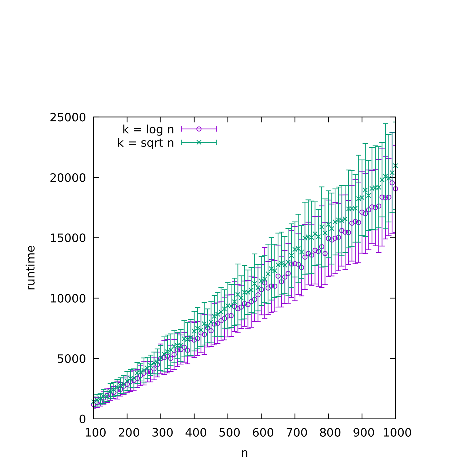
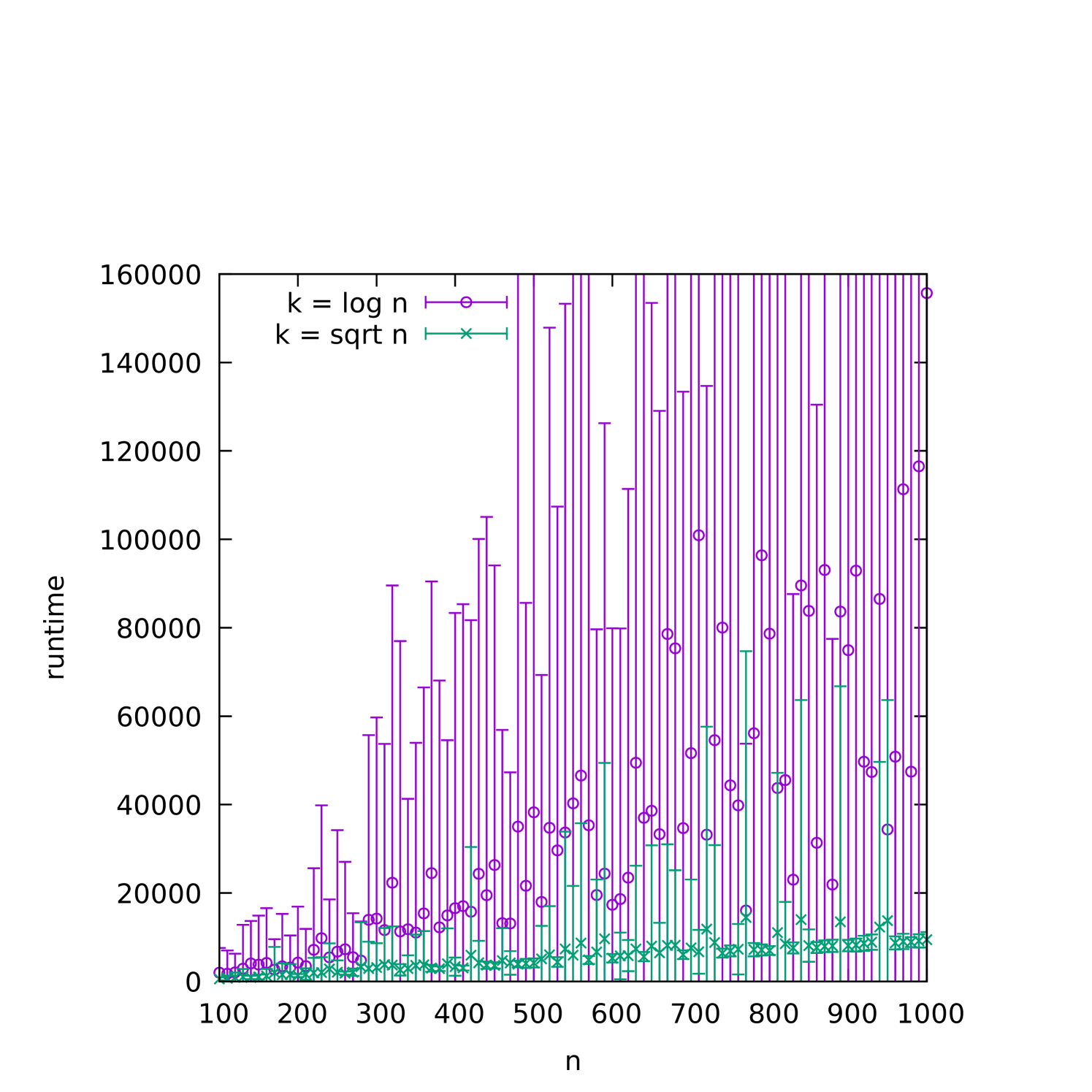
This scaling behavior is not so surprising, as we expect that random planted graphs are particularly easy for the (1+1) EA. Similar to the case of random planted satisfiability [DNS17], the relatively uniform structure of the problem is likely to provide a good fitness signal for hill-climbing type algorithms.

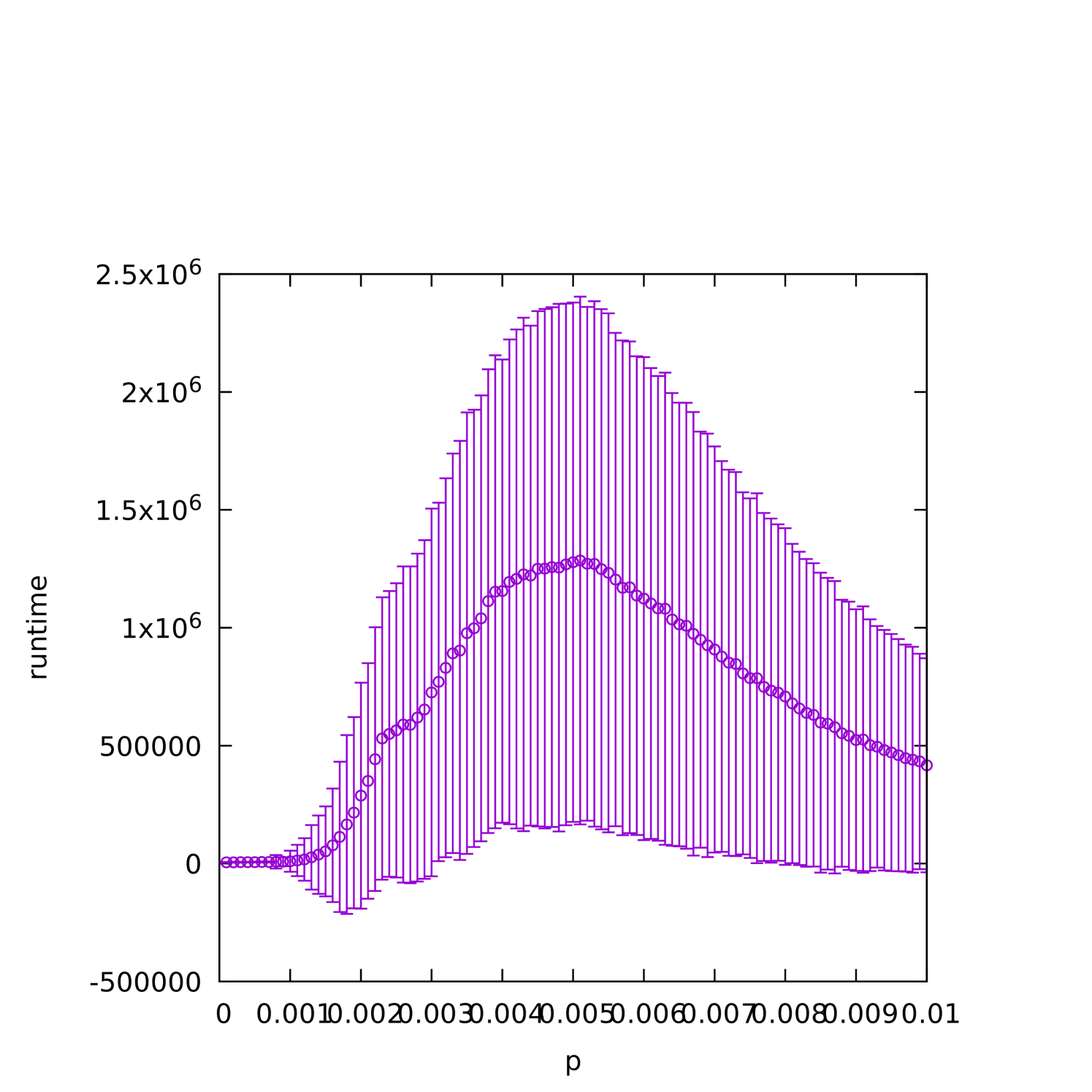
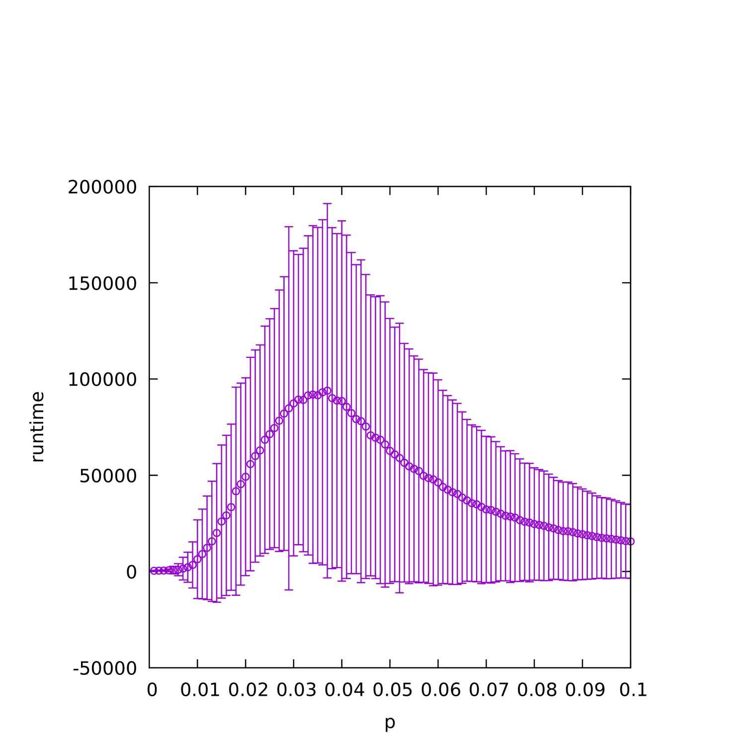
Random distributions of problems often undergo a so-called phase transition as various system parameters are varied. Very often, problems sampled near a critical density tend to be (empirically) harder to solve by different algorithms. For example, empirical evidence suggests critically-constrained planted propositional satisfiability formulas are difficult for the (1+1) EA when they are sampled near a critical density [DNS17]. To study the performance of the (1+1) EA on $\mathcal{G}{\left({n},{k},{p}\right)}$ as a function of graph density, we plot the dependence of the average runtime on $p$ in Figures 2(a) and 2(b), holding $n$ fixed and averaging over all values of $k$. We also see in this case a dependence on graph density in which the (1+1) EA performs worse in a band of not-too-sparse but not-too-dense graphs.

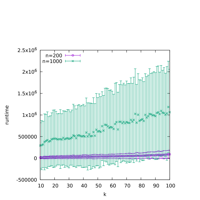
The dependence of runtime on $k$, however, is more uniform as we can see in Figure 3. Here we have aggregated over all $p$ values, which likely explains the large variance, especially in the larger $n=1000$ problems.

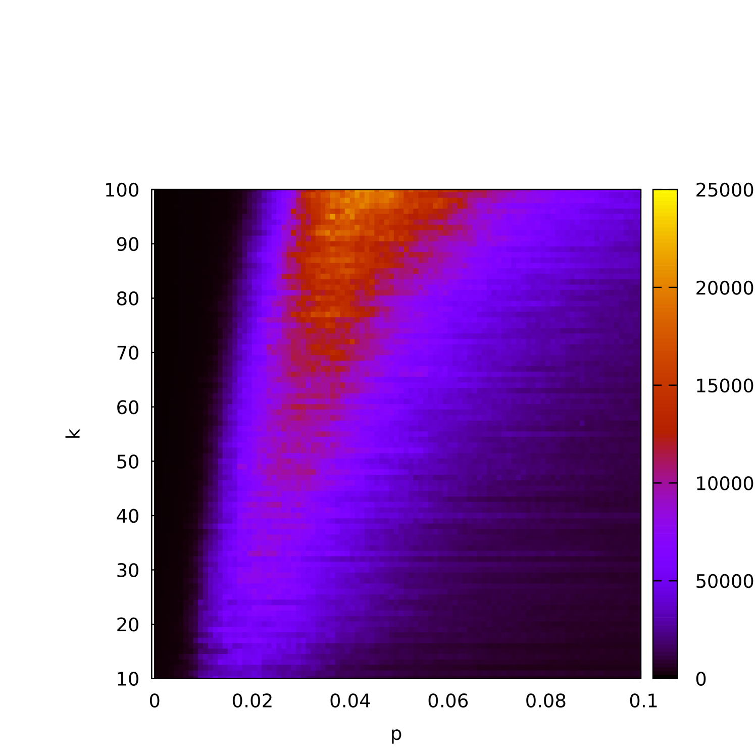
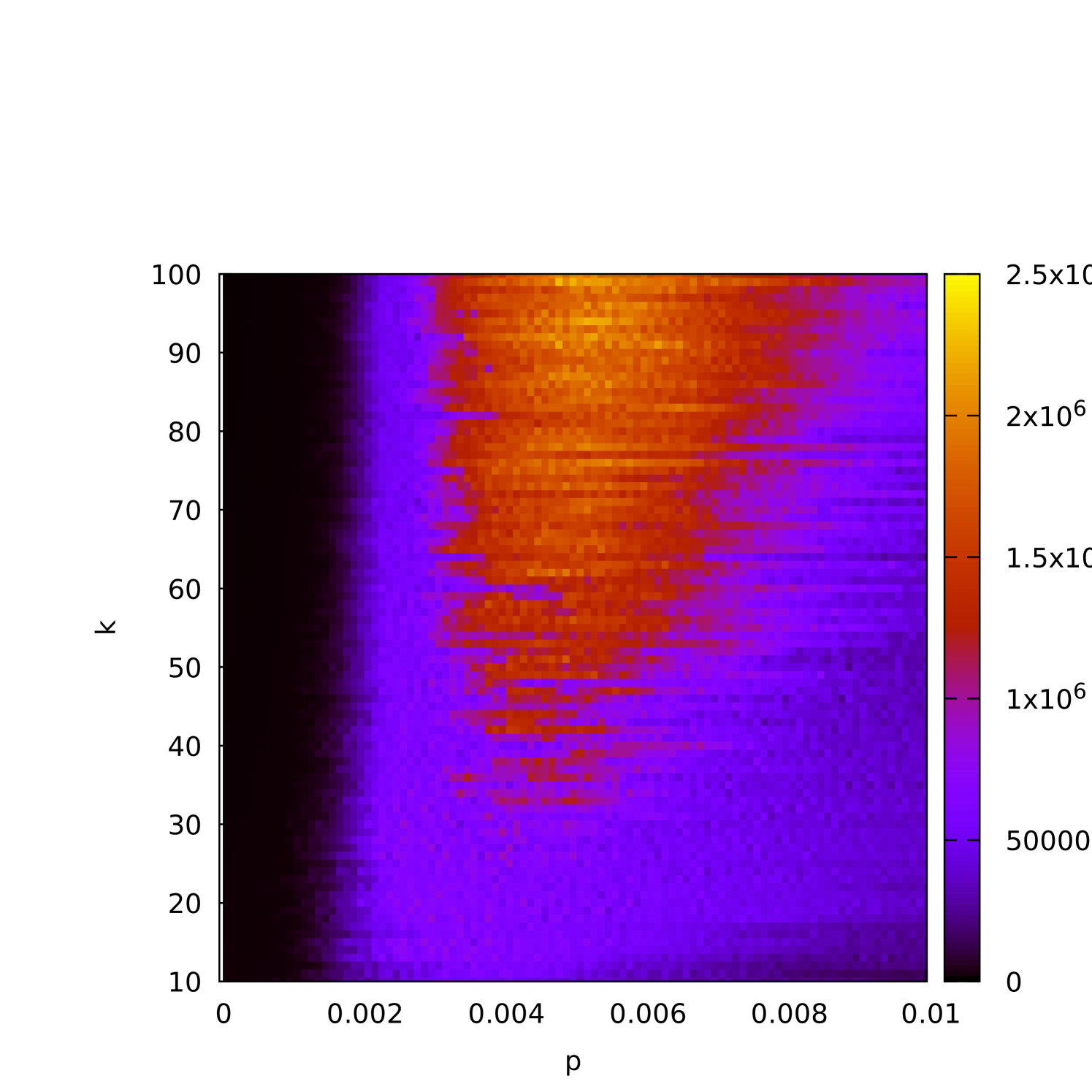
A more detailed picture is provided by Figures 4(a) and 4(b), where we display two-dimensional color plots showing the runtime dependence on both $k$ and $p$ simultaneously. On these plots one can see how the density and the cover size influences the efficiency of the (1+1) EA. We conjecture that there is a critical value (or range) of $p$ at which the (1+1) EA struggles to find a $k$-cover.

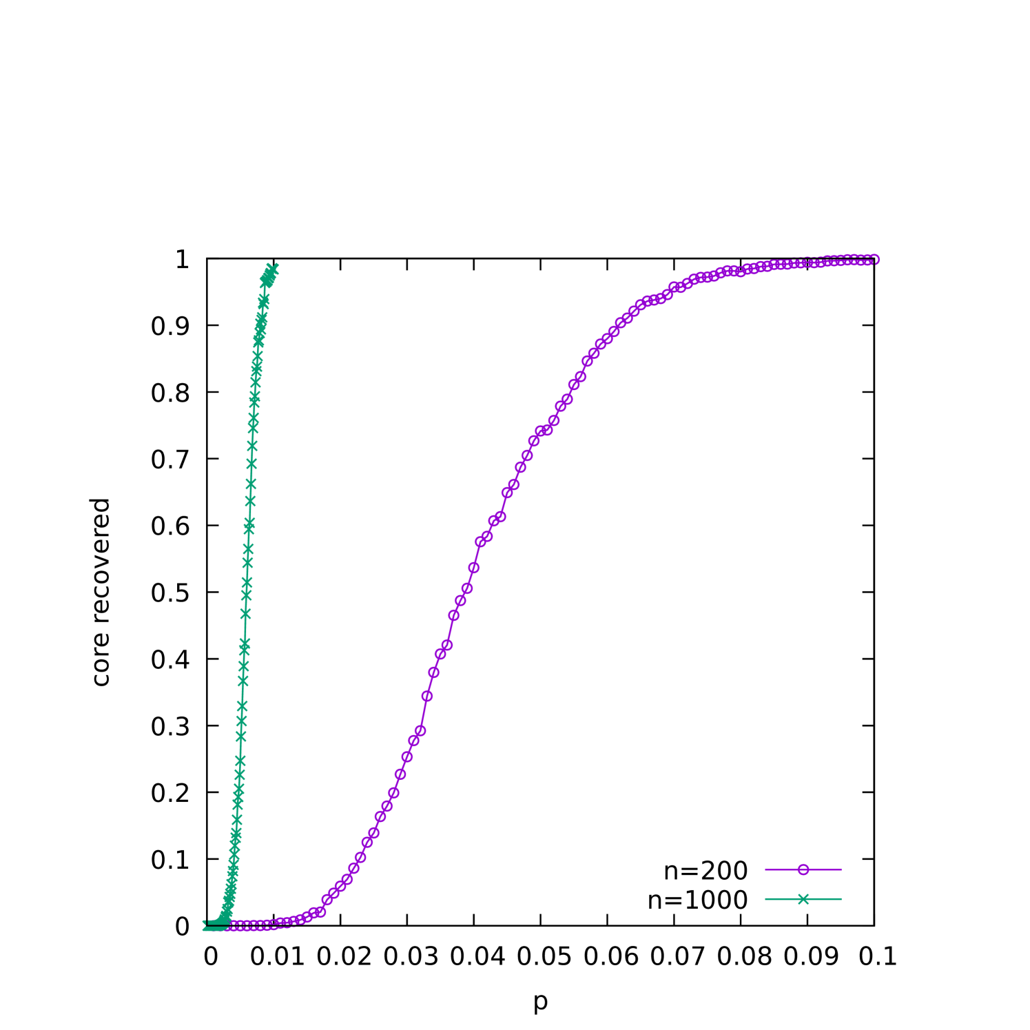
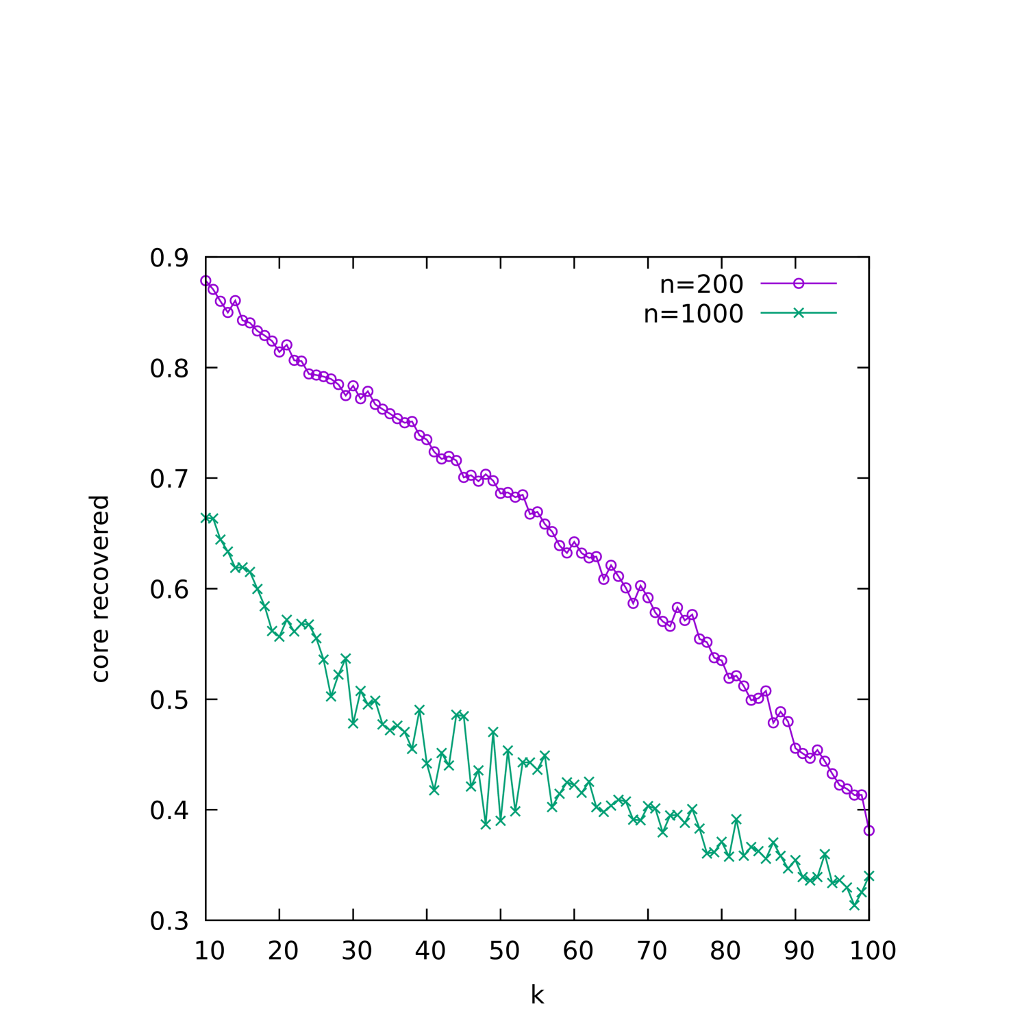
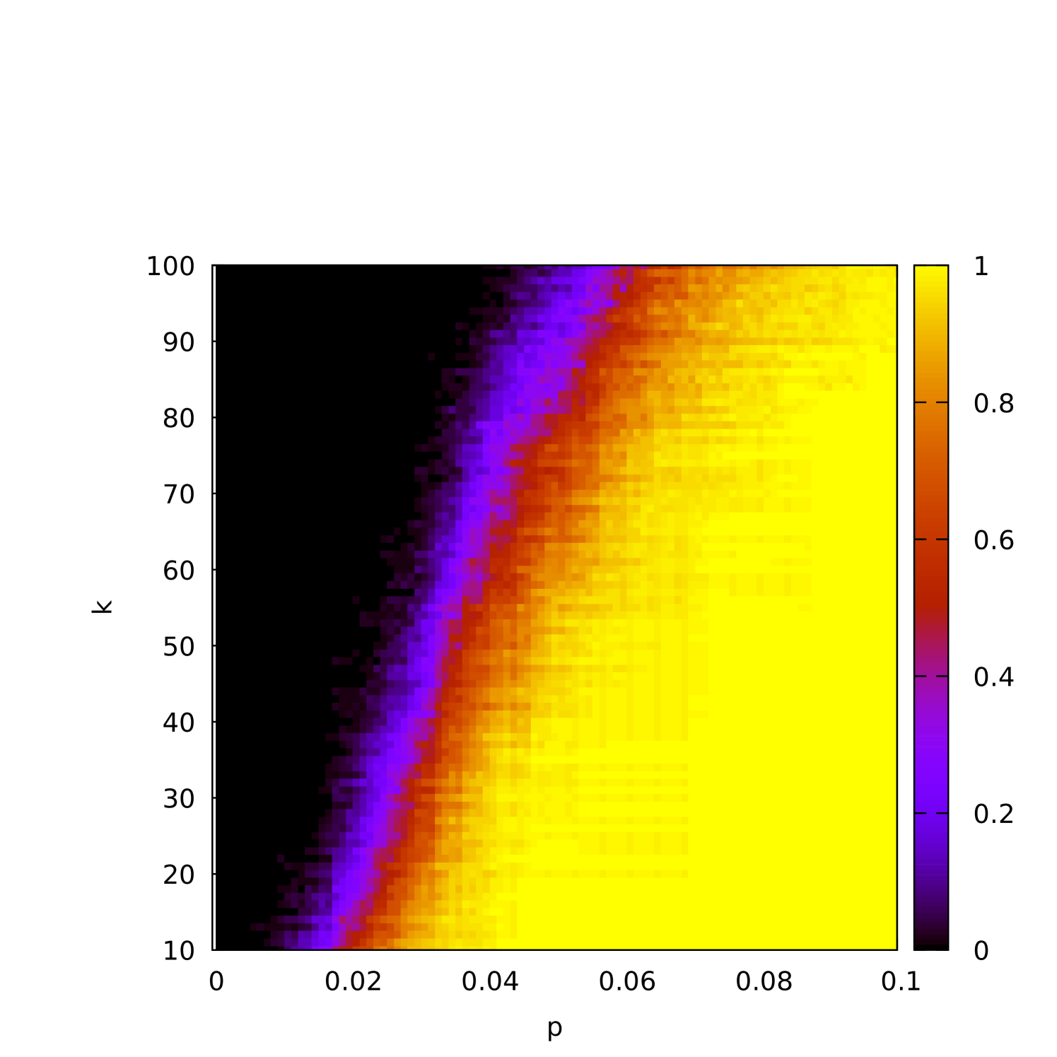
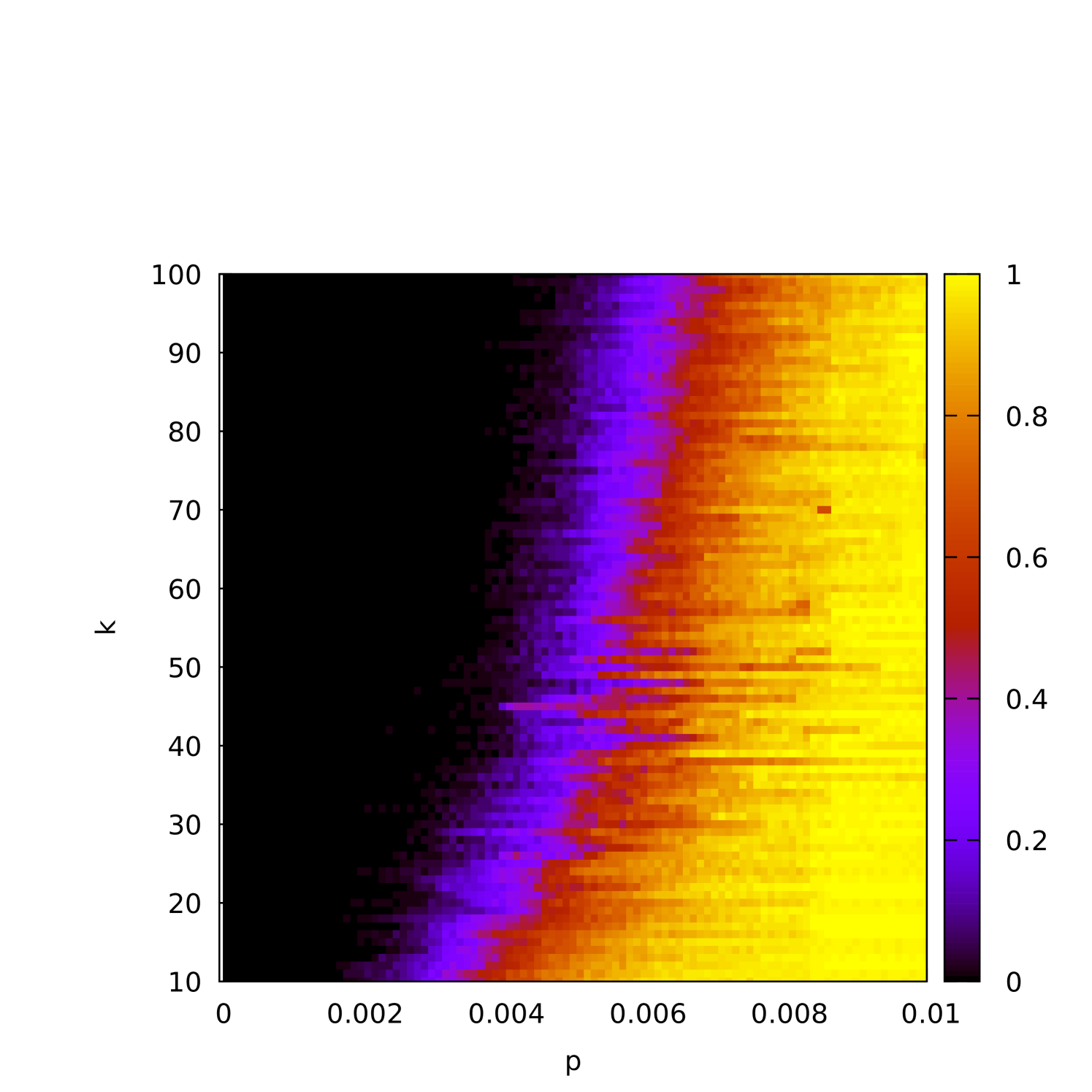
The (1+1) EA completes execution as soon as it finds a $k$-cover. However, this is not necessarily guaranteed to be the $k$-cover that was planted in the graph. Indeed, for smaller densities, we would expect many other $k$-covers in the graph. To investigate this, in Figure 5(a) we plot the proportion of runs in which the planted $k$-core was recovered (as opposed to some different $k$-cover) as a function of $p$. The dependence of this characteristic as a function of $k$ is plotted in Figure 5(b), and Figures 5(c) and 5(d) display this in a color plot for both $k$ and $p$ simultaneously.

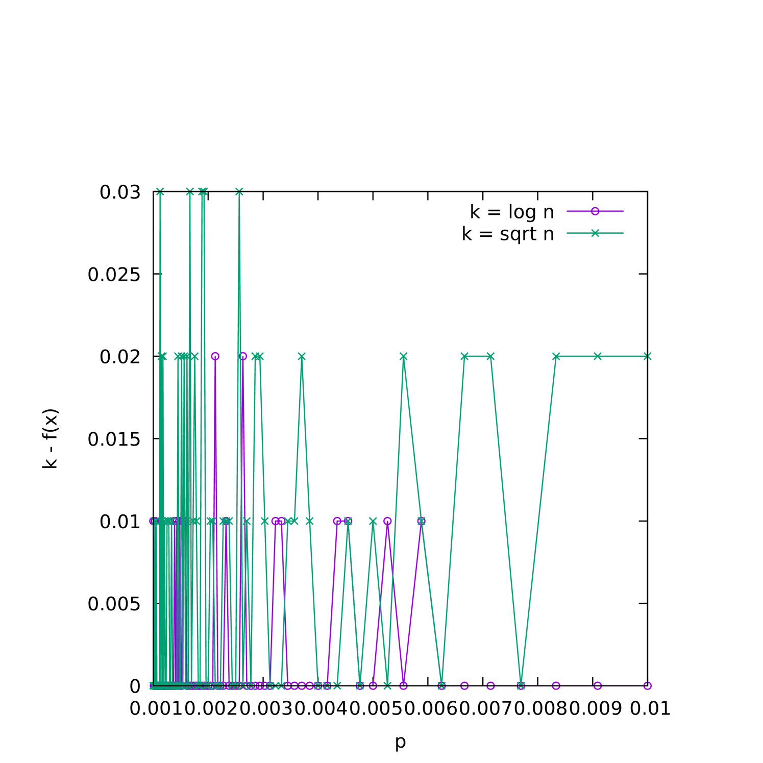
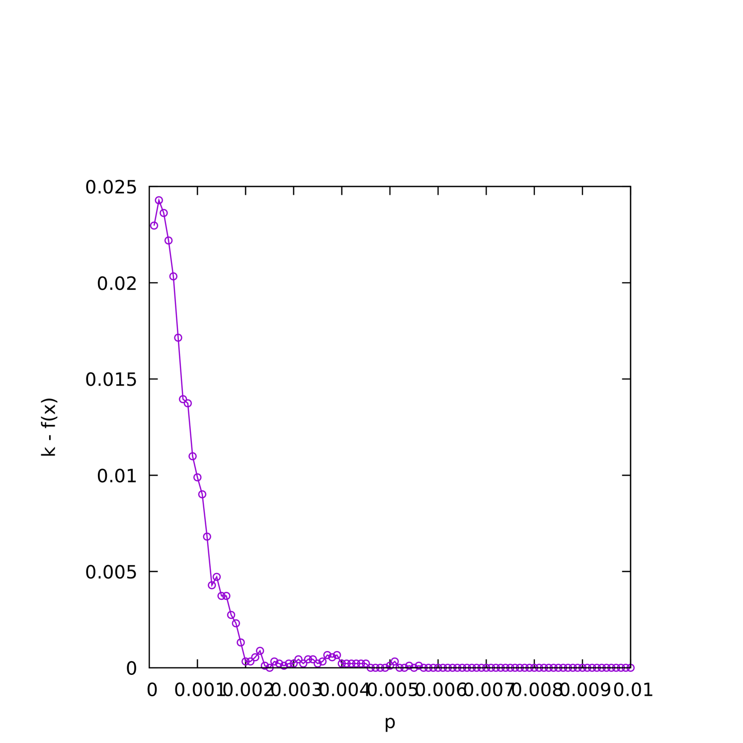
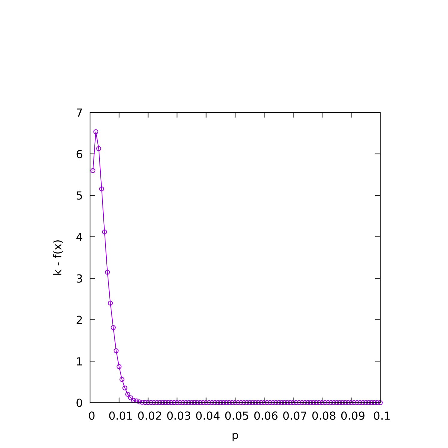
When the graph is relatively sparse, we would also expect the (1+1) EA to “overshoot” $k$ by finding an even smaller cover before finding a $k$-cover. To understand better how this depends on $k$ and $p$, we plot the average difference between $k$ and the best fitness found as a function of $p$ on sparse ($p=1/n$) instances where $n$ is varied in Figure 6(a), and on fixed-$n$ instances in Figures 6(b) and 6(c).

In this paper we have presented a parameterized analysis the (1+1) EA on problems drawn from the $\mathcal{G}{\left({n},{p},{k}\right)}$ random planted vertex cover model. We showed that for dense graphs $(p>0.71)$ and small $k$, there is sufficient signal in enough of the space so that the (1+1) EA has a relatively good chance of finding a $k$-cover in a polynomial-length run. When $k$ is large, we showed that a feasible cover cannot leave too much of the planted core uncovered, and therefore the (1+1) EA does not require a large effort to make progress. In the end, this translates to a fixed-parameter tractable runtime for the (1+1) EA with high probability over $\mathcal{G}{\left({n},{p},{k}\right)}$.

To fill in the picture, we also reported a number of computational experiments that measure the runtime on graphs drawn from $\mathcal{G}{\left({n},{p},{k}\right)}$. These experiments point to a critical value for $p$ at which the (1+1) EA requires more time to find any $k$-cover, which suggest an interesting direction for future theoretical work to understand this phenomenon better.

This work was supported by the National Science Foundation under grant 2144080 and by the Australian Research Council under grant FT200100536.

References

- [AKS98] Noga Alon, Michael Krivelevich, and Benny Sudakov. Finding a large hidden clique in a random graph. Random Structures & Algorithms, 13(3–4):457–466, 1998.
- [AS15] Emmanuel Abbe and Colin Sandon. Community detection in general stochastic block models: Fundamental limits and efficient algorithms for recovery. In 2015 IEEE 56th Annual Symposium on Foundations of Computer Science (FOCS), pages 670–688, 2015.
- [BFN+23] Samuel Baguley, Tobias Friedrich, Aneta Neumann, Frank Neumann, Marcus Pappik, and Ziena Zeif. Fixed parameter multi-objective evolutionary algorithms for the w-separator problem. In Genetic and Evolutionary Computation Conference (GECCO ’23), 2023.
- [BK18] Austin R. Benson and Jon M. Kleinberg. Found graph data and planted vertex covers. In Samy Bengio, Hanna M. Wallach, Hugo Larochelle, Kristen Grauman, Nicolò Cesa-Bianchi, and Roman Garnett, editors, Advances in Neural Information Processing Systems 31: Annual Conference on Neural Information Processing Systems 2018, NeurIPS 2018, December 3-8, 2018, Montréal, Canada, pages 1363–1374, 2018.
- [BS21] Luke Branson and Andrew M. Sutton. Focused jump-and-repair constraint handling for fixed-parameter tractable graph problems. In Proceedings of the 16th ACM/SIGEVO Conference on Foundations of Genetic Algorithms. Association for Computing Machinery, New York, NY, USA, 2021.
- [DG10] Benjamin Doerr and Leslie Ann Goldberg. Drift analysis with tail bounds. In Proceedings of the Eleventh International Conference on Parallel Problem Solving from Nature (PPSN XI), volume 6238 of Lecture Notes in Computer Science, pages 174–183. Springer, 2010.
- [DNS17] Benjamin Doerr, Frank Neumann, and Andrew M. Sutton. Time complexity analysis of evolutionary algorithms on random satisfiable k-CNF formulas. Algorithmica, 78(2):561–586, June 2017.
- [FHH+10] Tobias Friedrich, Jun He, Nils Hebbinghaus, Frank Neumann, and Carsten Witt. Approximating covering problems by randomized search heuristics using multi-objective models. Evolutionary Computation, 18(4):617–633, June 2010.
- [HLL83] Paul W. Holland, Kathryn Blackmond Laskey, and Samuel Leinhardt. Stochastic blockmodels: First steps. Social Networks, 5(2):109–137, 1983.
- [Hoe63] Wassily Hoeffding. Probability inequalities for sums of bounded random variables. Journal of the American Statistical Association, 58(301):13–30, 1963.
- [Jer92] Mark Jerrum. Large cliques elude the metropolis process. Random Structures & Algorithms, 3(4):347–359, 1992.
- [JOZ13] Thomas Jansen, Pietro S. Oliveto, and Christine Zarges. Approximating vertex cover using edge-based representations. In Frank Neumann and Kenneth A. De Jong, editors, Proceedings of the Twelfth Workshop on Foundations of Genetic Algorithms (FOGA XII), Adelaide, SA, Australia, January 16-20, 2013, pages 87–96. ACM, 2013.
- [JP00] Ari Juels and Marcus Peinado. Hiding cliques for cryptographic security. Designs, Codes and Cryptograrphy, 20(3):269–280, 2000.
- [KB94] Sami Khuri and Thomas Bäck. An evolutionary heuristic for the minimum vertex cover problem. In J. Kunze and H. Stoyan, editors, Workshops of the Eighteenth Annual German Conference on Artificial Intelligence (KI-94), Saarbrücken, Germany, pages 86–90, 1994.
- [KK19] Timo Kötzing and Martin S. Krejca. First-hitting times under drift. Theoretical Computer Science, 796:51–69, 2019.
- [KN12] Stefan Kratsch and Frank Neumann. Fixed-Parameter Evolutionary Algorithms and the Vertex Cover Problem. Algorithmica, 65(4):754–771, May 2012.
- [KR08] Subhash Khot and Oded Regev. Vertex cover might be hard to approximate to within . Journal of Computer and System Sciences, 74(3):335–349, 2008. Computational Complexity 2003.
- [MU05] Michael Mitzenmacher and Eli Upfal. Probability and Computing : Randomized Algorithms and Probabilistic Analysis. Cambridge University Press, 2005.
- [OHY09] Pietro S. Oliveto, Jun He, and Xin Yao. Analysis of the (1+1) EA for finding approximate solutions to vertex cover problems. IEEE Transactions on Evolutionary Computation, 13(5):1006–1029, 2009.
- [RUK19] Daniel M. Romero, Brian Uzzi, and Jon M. Kleinberg. Social networks under stress: Specialized team roles and their communication structure. ACM Trans. Web, 13(1):6:1–6:24, 2019.
- [Sto07] Tobias Storch. Finding large cliques in sparse semi-random graphs by simple randomized search heuristics. Theoretical Computer Science, 386:114–131, 2007.